Analytical Calculation
of Two-Loop Feynman Diagrams
R. Bonciani111Email:
Roberto.Bonciani@physik.uni-freiburg.de
222Presented at the final meeting of the European Network
“Physics at Colliders”, Montpellier, September 26-27 2004
Fakultät für Mathematik und Physik, Albert-Ludwigs-Universität
Freiburg,
D-79104 Freiburg, Germany
We review the Laporta algorithm for the reduction of scalar integrals to the master integrals and the differential equations technique for their evaluation. We discuss the use of the basis of harmonic polylogarithms for the analytical expression of the results and some generalization of this basis to wider sets of transcendental functions.
1 Introduction
In the last few years a large amount of work has been devoted to the improvement of the techniques for the calculation of Feynman diagrams. The reason is that future high energy physics experiments will reach a measurement precision that will require, from the theoretical counterpart, the control on the NNLO quantum corrections for several physical observables.
Basically two approaches have been developed for the calculation of Feynman diagrams: the first one is based on the numerical and the other on the analytical evaluation of the integrals involved. The goal of both approaches is the complete and “automatic” evaluation of Feynman diagrams in multi-scale processes, but, nowadays, this goal is far from being achieved. Different problems arise. While for the numerical approach the presence of different scales is not a problem, the treatment of infrared singularities, thresholds and pseudo-thresholds is of complicated solution and sometimes it has to be performed in a semi-analytic way. On the other hand, the analytic approach gives a complete control on the “difficult” regions of the spectrum, but it is, at the moment, constrained to processes in which the scales in the game are at most three.
Nevertheless, in both cases great results have been obtained.
In [1] a semi-numerical approach to the calculation of two-loop Feynman diagrams was proposed and applied to the two-loop self-energy of the Higgs boson and to the decay ; in [2] a method based on the Bernstein-Tkachov theorem was proposed and applied both to multi-leg one-loop and to two-point and three-point two-loop Feynman diagrams. In [3] a numerical method based on the sector decomposition was proposed and applied to multi-leg one-loop Feynman diagrams calculations as well as to two-loop and three-loop two-, three- and four-point functions in the non-physical region and to the evaluation of phase-space integrals. Finally, in [4] the numerical evaluation of two-point functions was made by means of differential equations solved with the Runge-Kutta method.
For what concerns the analytical approach, the evaluation of vacuum diagrams, two-point, three-point and four-point functions (see for example [5], [6, 11, 16, 27], and [7, 10, 29]), used also in the case of phase-space integrals (see [8]), was made, in the last few years, with a variety of different techniques. Since [9], the most used one consists in the reduction of the Feynman diagrams to a small set of scalar integrals, via integration-by-parts, Lorentz-invariance [10] and general symmetry identities [11], followed by the calculation of the scalar integrals with different methods such as, for example, the expansion by regions [12], the Mellin-Barnes transformations [13], the relations among integrals of different dimension [14], or the differential equations method [15].
In this paper we will review the algorithm for the reduction of the Feynman diagrams to the set of independent scalar integrals, called Master Integrals (MIs) and the differential equations technique for their evaluation. The problem of the choice of the basis of functions used for the expression of the analytical results will be also discussed, giving particular emphasis to the Harmonic Polylogarithms and the several extensions that took place recently.
2 Algebraic Reduction to Master Integrals
The calculation of a physical observable for a certain reaction in perturbation theory is connected to the evaluation of the Feynman diagrams involved in the process. Once the observable is written in terms of Feynman diagrams and the Dirac algebra is performed (that means usually that the traces over the Dirac indices are evaluated), we find an expression which is a combination of (several) scalar integrals, whose ultraviolet and infrared divergences are regularized within the dimensional regularization scheme. The general structure of such integrals at the 2-loop level is the following:
| (1) |
where is the number of different denominators (this number is called topology of the integral), is the number of independent scalar products on the numerator, and stands for a suitable integration measurement (normalization) for the integrals.
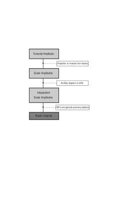
The reduction of the integrals of Eq. (1) to the MIs is schematically represented in the flowchart of Fig. 1 and it is based on the following steps:
-
1.
Once the Feynman diagrams for the evaluation of the observable are written, we project the corresponding amplitude on a basis of known tensors in such a way that the amplitude can be written in terms of scalar form factors. These form factors are expressed in terms of a huge number of scalar integrals, that can have on the numerator a combination of scalar products between an external momentum and a loop-momentum or between two loop-momenta; note that, because we use dimensional regularization, a simplification between a scalar product and a denominator that contains this scalar product is possible. Once a denominator disappears, because of the simplification against a scalar product, the topology of the integral is of course lowered by a unit. In principle, given an integral of topology , one must consider all the possible subtopologies found simplifying repeatedly a denominator against a scalar product on the numerator.
-
2.
The scalar integrals are classified with respect to their topology. Because we are dealing with integrals that have a suitable mass distribution (for example we can consider integrals with mass-less propagators and outgoing legs) it can happen that subtopologies coming from different simplifications are the same subtopology, but expressed with different routings. Therefore, the “independent” subtopologies have to be chosen and the “dependent” subtopologies have to be transformed by means of suitable transformations in the independent ones. This analysis can be done in the framework of the “Auxiliary diagram scheme” or the “shifts scheme”, as explained extensively in [16].
-
3.
The reduction of the scalar integrals belonging to the independent topologies to a “hopefully” small set of master integrals (MIs), is done by means of the so-called Laporta algorithm [17], which consists in the following. We know that the -regularized scalar integrals coming from the projection operation are not all independent, but they satisfy certain classes of identity relations.
-
•
The most important class is constituted by the integration-by-part identities (IBPs), introduced in [9]. IBPs link scalar integrals of the same topology, but with different power of the denominator and different scalar products on the numerator, among each other and to scalar integrals of subtopologies. IBPs can be written in the following way:
(2) where and where is one of the independent vector of the problem. In the case of a 3-point functions, Eq. (2) gives 8 equations for initial scalar amplitude in the brackets. For a 4-point function, instead, the IBPs are 10.
-
•
Another class of identity relations that can be used in the reduction process is related to the fact that the integrals are Lorentz scalars [10]. This property translates into one additional equation for a 3-point function:
(3) where and are the independent vectors of the problem, or three additional equations for a 4-point function:
(4) (5) (6) where the independent vectors are , and .
-
•
In the case in which a suitable mass distribution is considered, we can find additional equations considering the symmetries of the diagrams (see [11]). In general a symmetry of the problem brings to an identity that the integrals have to satisfy.
Considering all the identity relations mentioned above, a huge system of linear equations is constructed. The unknowns are the scalar integrals themselves and the point is that the construction of the system can give more equations than unknown amplitudes [17], overconstraining formally the system; but not all the equations are independent. It can happen that the system is effectively overconstrained, and then the solution of the system gives the integrals of the topology under consideration as a combination of the MIs of the subtopologies, or it is not, and then all the integrals of the topology under consideration are expressed as a combination of the MIs of that topology (and the MIs of the subtopologies). The solution of the system is performed with the Gauss law of substitution. The entire chain is completely algebraic and can be implemented in a computer program.
-
•
Several authors developed own programs, written in FORM [18], C, or Mathematica [19], for the generation of the linear system and for its solution [20, 21]. Recently, a computer program written for Maple [22], using the Laporta algorithm for the reduction of scalar integrals to the MIs was published [23].
3 The Differential Equations Method
The MIs are functions of the external kinematical invariants and, therefore, they satisfy a system of first-order linear differential equations. As a simple example, consider the case in which a topology has a single MI. Let us choose the basic scalar integral of the topology333The choice of the set of MIs to which all the scalar integrals belonging to a certain topology can be reduced is totally free. One choice is connected to another by the identity relations constructed for the reduction process. A criterion in the preference of one set with respect to the others is, of course, related to the solution of the system of differential equations. We choose the set that satisfy the easiest possible system. That means, usually, the set for which the system is decoupled exactly in or at least triangularizes in the limit .:
| (7) |
where stand for the independent invariants that can be constructed with the external momenta of the problem (for example , , etc.).
The following matrix can be constructed:
| (8) |
As depends on the invariants , we have, on one hand:
| (9) |
where the functions are linear combinations of . On the other hand, because is evaluated in dimensional regularization, and then it is convergent, we can perform the derivative of Eq. (8) directly on the integrand , getting a combination of scalar integrals with additional power on the denominator and scalar products on the numerator. Using the identity relations loaded for the reduction to the MIs, the system of Eq. (8) becomes a linear system involving the derivatives of with respect to the invariants , itself and the MIs of the subtopologies. The system can be inverted and the differential equations can be written in the following general way:
| (10) |
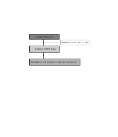
where the non-homogeneous term contains the MIs of the subtopologies, that have to be considered known. The homogeneous term gives the analytical structure of the function , containing the thresholds and pseudo-thresholds of the diagram under consideration, that appear as singular points for the differential equation444The construction of the system of first-order linear differential equations is outlined in the flowchart of Fig. 2.. Note that one of the differential equations is sufficient for the solution of , provided that we are able to fix the boundary conditions. Therefore, we can consider only the equation with respect to, say, . The solution of Eq. (10) is done by means of the Euler’s method of variation of the arbitrary constants.
We can sketch the search for the solution as follows:
-
1.
We expand (the dependence on the other invariants is understood) in Laurent series of :
(11) where is the maximum pole and is the required order in needed for . Order by order in we have, then, to solve the equation:
(12) where for (the maximum pole) we have ( is the non-homogeneous part in Eq. (10)) and for , can involve also the previous orders in of . Note that, while the non-homogeneous term is different at each order in , the homogeneous equation is the same.
-
2.
We solve the homogeneous equation
(13) finding the solution:
(14) -
3.
We express the solution of the non-homogeneous equation order by order in in the integral form:
(15) where is the arbitrary constant of integration.
-
4.
We fix the constant of integration imposing the initial conditions. In order to find the initial conditions we have to know additional pieces of information about the integral we are calculating. For example it is sufficient to know that the integral is regular for some value of .
In the case of MIs () we have still a system of first-order coupled linear differential equations for every variable . As in the previous case the equations in one of the invariants are sufficient for the solution.
In spite of the elegance of the method, two problems arise.
One is connected with the number of MIs that a topology can have. In fact, while the solution of a first-order linear differential equation (case with one MI) is relatively trivial, a second-order differential equation (case with two MIs) can give more problems and starting from the third-order one it can be hard to find the solution, except in very particular cases. We can understand, therefore, the importance of the choice of the set of MIs. A choice that, even in the case of two or more MIs, could triangularize the system, at least in the expansion, would be of course more suitable than another; but this choice can not always be done and, in general, there is not always a solution for the problem of a topology with many MIs.
Another problem concerns the choice of the basis of functions used for the expression of the analytical results. Even in this case, there is not a unique solution, but, nevertheless, one can follow some guidelines. For example the uniqueness of the representation of the result in terms of these functions; the non-redundancy of the representation and the absence of “hidden zeroes” (that means to avoid representations that can give expressions that are not manifestly zero, but, because of the fact that these functions satisfy certain relations, they are effectively zero); the total control on the expansions in all the points of the domain and on the analytical continuation (these two “properties” are needed for a numerical evaluation of the functions and then of the result).
All these properties are fulfilled, by construction, by the set of functions called Harmonic Polylogarithms, that we are going to review briefly in the next paragraph.
4 Harmonic Polylogarithms and Related Generalized Functions
In many cases, a suitable integral representation for the Feynman diagrams can be found in terms of hypergeometric functions. Nevertheless, in problems involving many scales, the dependence of the generalized hypergeometric functions on these scales is highly non-trivial. Moreover, if we regularize the divergent integrals in dimensional regularization, an expansion in is required, for renormalization purposes. The expansion of a hypergeometric function in its parameters can be very complicated [24]. This is the reason why one looks for a solution of the differential equations directly expanded in . Order by order in , we can find a representation for the MIs in terms of Nielsen’s polylogarithms and related functions [25]. But, firstly, the representation in terms of polylogarithms suffers from the problem of “hidden zeroes” discussed at the end of the previous paragraph; moreover, it can happen that one needs an integral representation that does not belong to this class of functions.
One of the most elegant solutions for these two problems is the introduction of a basis of transcendental functions defined by repeated integration over a set of basic simple functions. Let us consider for example a case in which we have at most two different scales in the problem, say and , in such a way that we can construct the dimensionless parameter ; moreover, the structure of the thresholds of the Feynman diagrams involved in the calculation is such that the possible singular points are and and no squared roots are present in the homogeneous equation for the MIs (this is actually the case of the majority of the calculations in [5, 6, 11, 16, 27]). In this situation a suitable basis of functions in which the results can be expressed are the 1-dimensional harmonic polylogarithms (HPLs) introduced in [26]. We consider the following set of three basis functions:
| (16) |
we define the HPLs of weight 1 as:
| (17) | |||||
| (18) | |||||
| (19) |
and we iterate the previous definition introducing the HPLs of weight
| (20) |
where can take the values -1, 0 and 1 and is a vector with components, consisting of a sequence of -1, 0 and 1 as well.
The set of functions so defined satisfy two important properties: i. they form a shuffle algebra, in which the product of two HPLs of weight and is a HPL of weight ; ii. they form a closed set under certain transformations of the argument. In particular, this property is needed for the asymptotic evaluation of such a functions, connecting the expansion in to the one in . Another important property of HPLs is that their analytical structure is manifestly shown. The integral representations of Eq. (15) can be expressed in terms of HPLs directly or re-conducted to HPLs via simple integration by parts.
The choice of the basis (16) for the expression of the HPLs is connected with the structure of the thresholds of the diagrams involved in the calculation. It can happen that the solution of the homogeneous differential equation contains a square root, that can not be avoided by a suitable change of variables. Moreover, we can deal with a calculation in which, for example, the diagrams can have three different kind of thresholds: , and . In this case an extension of the basis of HPLs is needed [27]. We introduce the following additional basis functions:
| (21) |
The relative weight-1 HPLs are defined as the integration between 0 and of the previous basis functions (all the functions in Eq. (21) are integrable in ) and the generalization to higher weights is done by Eq. (20) in which now the single weight can take the values 0, , , , , , , , , .
The set of generalized HPLs so introduced satisfy all the properties of the former set of HPLs. Similar generalizations can be carried out in the case of different thresholds.
Another generalization can be done in the case in which we have three scales in the game and, therefore, two dimensionless parameters can be constructed. This gives the so-called 2-dimensional HPLs introduced in [28, 29] and their further extension introduced in [30].
As a remark, note that the representation of the analytical results in terms of HPLs allows a perfect control on the numerical evaluations.
5 Summary
In this paper the Laporta algorithm for the reduction of the Feynman diagrams to the master integrals and the differential equations technique for their analytical evaluation are reviewed. A particular attention is paid to the problem of the choice of the basis of functions in which the result can be expressed. Some argument for the use of HPLs is done. In particular, the possibility of an extension of the set of functions to the case of problems involving different thresholds and different scales (more than two) is briefly outlined.
References
-
[1]
A. Ghinculov and J. J. van der Bij,
Nucl. Phys. B 436 (1995) 30
[arXiv:hep-ph/9405418].
A. Ghinculov and Y. P. Yao, Nucl. Phys. B 516 (1998) 385 [arXiv:hep-ph/9702266].
A. Ghinculov and Y. P. Yao, Phys. Rev. D 63 (2001) 054510 [arXiv:hep-ph/0006314].
A. Ghinculov and Y. P. Yao, in Proc. of the 5th International Symposium on Radiative Corrections (RADCOR 2000) ed. Howard E. Haber, arXiv:hep-ph/0106020. -
[2]
G. Passarino,
Nucl. Phys. B 619 (2001) 257
[arXiv:hep-ph/0108252].
G. Passarino and S. Uccirati, Nucl. Phys. B 629 (2002) 97 [arXiv:hep-ph/0112004].
A. Ferroglia, M. Passera, G. Passarino and S. Uccirati, Nucl. Phys. B 650 (2003) 162 [arXiv:hep-ph/0209219].
A. Ferroglia, G. Passarino, S. Uccirati and M. Passera, Nucl. Instrum. Meth. A 502 (2003) 391.
A. Ferroglia, M. Passera, G. Passarino and S. Uccirati, Nucl. Phys. B 680 (2004) 199 [arXiv:hep-ph/0311186].
S. Actis, A. Ferroglia, G. Passarino, M. Passera and S. Uccirati, arXiv:hep-ph/0402132. -
[3]
T. Binoth and G. Heinrich,
Nucl. Phys. B 585 (2000) 741
[arXiv:hep-ph/0004013].
T. Binoth, G. Heinrich and N. Kauer, Nucl. Phys. B 654 (2003) 277 [arXiv:hep-ph/0210023].
T. Binoth and G. Heinrich, Nucl. Phys. B 680 (2004) 375 [arXiv:hep-ph/0305234].
T. Binoth and G. Heinrich, Nucl. Phys. B 693 (2004) 134 [arXiv:hep-ph/0402265].
T. Binoth, arXiv:hep-ph/0407003.
G. Heinrich, arXiv:hep-ph/0406332. -
[4]
M. Caffo, H. Czyz and E. Remiddi,
Nucl. Phys. B 634 (2002) 309
[arXiv:hep-ph/0203256].
M. Caffo, H. Czyz and E. Remiddi, Nucl. Instrum. Meth. A 502 (2003) 613 [arXiv:hep-ph/0211171].
M. Caffo, H. Czyz, A. Grzelinska and E. Remiddi, Nucl. Phys. B 681 (2004) 230 [arXiv:hep-ph/0312189]. -
[5]
D. J. Broadhurst,
Z. Phys. C 47 (1990) 115.
A. I. Davydychev and J. B. Tausk, Nucl. Phys. B 397 (1993) 123.
D. J. Broadhurst, J. Fleischer and O. V. Tarasov, Z. Phys. C 60 (1993) 287 [arXiv:hep-ph/9304303].
A. I. Davydychev, V. A. Smirnov and J. B. Tausk, Nucl. Phys. B 410 (1993) 325 [arXiv:hep-ph/9307371].
R. Scharf and J. B. Tausk, Nucl. Phys. B 412 (1994) 523.
A. I. Davydychev and J. B. Tausk, arXiv:hep-ph/9504432.
A. I. Davydychev and J. B. Tausk, Nucl. Phys. B 465 (1996) 507 [arXiv:hep-ph/9511261].
T. van Ritbergen, J. A. M. Vermaseren and S. A. Larin, Phys. Lett. B 400 (1997) 379 [arXiv:hep-ph/9701390].
T. van Ritbergen and R. G. Stuart, Phys. Rev. Lett. 82 (1999) 488 [arXiv:hep-ph/9808283].
J. Fleischer, M. Y. Kalmykov and A. V. Kotikov, Phys. Lett. B 462 (1999) 169 [arXiv:hep-ph/9905249].
K. Melnikov and T. van Ritbergen, Nucl. Phys. B 591 (2000) 515 [arXiv:hep-ph/0005131].
A. I. Davydychev and M. Y. Kalmykov, Nucl. Phys. B 605 (2001) 266 [arXiv:hep-th/0012189].
M. Argeri, P. Mastrolia and E. Remiddi, Nucl. Phys. B 631 (2002) 388 [arXiv:hep-ph/0202123].
M. Awramik, M. Czakon, A. Onishchenko and O. Veretin, Phys. Rev. D 68 (2003) 053004 [arXiv:hep-ph/0209084].
P. Mastrolia and E. Remiddi, Nucl. Phys. B 657 (2003) 397 [arXiv:hep-ph/0211451].
M. Awramik and M. Czakon, Phys. Lett. B 568 (2003) 48 [arXiv:hep-ph/0305248].
S. Laporta, P. Mastrolia and E. Remiddi, Nucl. Phys. B 688 (2004) 165 [arXiv:hep-ph/0311255].
S. Laporta and E. Remiddi, arXiv:hep-ph/0406160. -
[6]
N. I. Usyukina and A. I. Davydychev,
Phys. Atom. Nucl. 56 (1993) 1553
[Yad. Fiz. 56N11 (1993) 172]
[arXiv:hep-ph/9307327].
N. I. Usyukina and A. I. Davydychev, Phys. Lett. B 332 (1994) 159 [arXiv:hep-ph/9402223].
N. I. Usyukina and A. I. Davydychev, Phys. Lett. B 348 (1995) 503 [arXiv:hep-ph/9412356].
J. Fleischer, V. A. Smirnov, A. Frink, J. G. Korner, D. Kreimer, K. Schilcher and J. B. Tausk, Eur. Phys. J. C 2 (1998) 747 [arXiv:hep-ph/9704353].
J. Fleischer, A. V. Kotikov and O. L. Veretin, Phys. Lett. B 417 (1998) 163 [arXiv:hep-ph/9707492].
J. Fleischer and M. Tentyukov, arXiv:hep-ph/9802244.
R. V. Harlander, Phys. Lett. B 492 (2000) 74 [arXiv:hep-ph/0007289].
A. I. Davydychev and V. A. Smirnov, Nucl. Instrum. Meth. A 502 (2003) 621 [arXiv:hep-ph/0210171].
P. Mastrolia and E. Remiddi, Nucl. Phys. B 664 (2003) 341 [arXiv:hep-ph/0302162].
R. Bonciani, P. Mastrolia and E. Remiddi, Nucl. Phys. B 676 (2004) 399 [arXiv:hep-ph/0307295].
R. Bonciani, P. Mastrolia and E. Remiddi, Nucl. Phys. B 690 (2004) 138 [arXiv:hep-ph/0311145].
J. Fleischer, O. V. Tarasov and V. O. Tarasov, Phys. Lett. B 584 (2004) 294 [arXiv:hep-ph/0401090].
U. Aglietti, R. Bonciani, G. Degrassi and A. Vicini, Phys. Lett. B 595 (2004) 432 [arXiv:hep-ph/0404071].
W. Bernreuther, R. Bonciani, T. Gehrmann, R. Heinesch, T. Leineweber, P. Mastrolia and E. Remiddi, arXiv:hep-ph/0406046.
U. Aglietti, R. Bonciani, G. Degrassi and A. Vicini, Phys. Lett. B 600 (2004) 57 [arXiv:hep-ph/0407162].
M. Awramik, M. Czakon, A. Freitas and G. Weiglein, arXiv:hep-ph/0407317. -
[7]
N. I. Usyukina and A. I. Davydychev,
Phys. Lett. B 298 (1993) 363.
V. A. Smirnov, Phys. Lett. B 460 (1999) 397 [arXiv:hep-ph/9905323].
V. A. Smirnov and O. L. Veretin, Nucl. Phys. B 566 (2000) 469 [arXiv:hep-ph/9907385].
J. B. Tausk, Phys. Lett. B 469 (1999) 225 [arXiv:hep-ph/9909506].
C. Anastasiou, E. W. N. Glover and C. Oleari, Nucl. Phys. B 575 (2000) 416 [Erratum-ibid. B 585 (2000) 763] [arXiv:hep-ph/9912251].
Z. Bern, L. J. Dixon and D. A. Kosower, JHEP 0001 (2000) 027 [arXiv:hep-ph/0001001].
C. Anastasiou, T. Gehrmann, C. Oleari, E. Remiddi and J. B. Tausk, Nucl. Phys. B 580 (2000) 577 [arXiv:hep-ph/0003261].
V. A. Smirnov, Phys. Lett. B 491 (2000) 130 [arXiv:hep-ph/0007032].
T. Gehrmann and E. Remiddi, Nucl. Phys. B 601 (2001) 248 [arXiv:hep-ph/0008287].
Z. Bern, L. J. Dixon and A. Ghinculov, Phys. Rev. D 63 (2001) 053007 [arXiv:hep-ph/0010075].
C. Anastasiou, E. W. N. Glover, C. Oleari and M. E. Tejeda-Yeomans, Nucl. Phys. B 601 (2001) 318 [arXiv:hep-ph/0010212].
V. A. Smirnov, Phys. Lett. B 500 (2001) 330 [arXiv:hep-ph/0011056].
C. Anastasiou, E. W. N. Glover, C. Oleari and M. E. Tejeda-Yeomans, Nucl. Phys. B 601 (2001) 341 [arXiv:hep-ph/0011094].
C. Anastasiou, E. W. N. Glover, C. Oleari and M. E. Tejeda-Yeomans, Phys. Lett. B 506 (2001) 59 [arXiv:hep-ph/0012007].
T. Gehrmann and E. Remiddi, Nucl. Phys. B 601 (2001) 287 [arXiv:hep-ph/0101124].
C. Anastasiou, E. W. N. Glover, C. Oleari and M. E. Tejeda-Yeomans, Nucl. Phys. B 605 (2001) 486 [arXiv:hep-ph/0101304].
E. W. N. Glover, C. Oleari and M. E. Tejeda-Yeomans, Nucl. Phys. B 605 (2001) 467 [arXiv:hep-ph/0102201].
E. W. N. Glover and M. E. Tejeda-Yeomans, JHEP 0105 (2001) 010 [arXiv:hep-ph/0104178].
Z. Bern, A. De Freitas and L. J. Dixon, JHEP 0109 (2001) 037 [arXiv:hep-ph/0109078].
Z. Bern, A. De Freitas, L. J. Dixon, A. Ghinculov and H. L. Wong, JHEP 0111 (2001) 031 [arXiv:hep-ph/0109079].
V. A. Smirnov, Phys. Lett. B 524 (2002) 129 [arXiv:hep-ph/0111160].
L. W. Garland, T. Gehrmann, E. W. N. Glover, A. Koukoutsakis and E. Remiddi, Nucl. Phys. B 627 (2002) 107 [arXiv:hep-ph/0112081].
Z. Bern, A. De Freitas and L. J. Dixon, JHEP 0203 (2002) 018 [arXiv:hep-ph/0201161].
L. W. Garland, T. Gehrmann, E. W. N. Glover, A. Koukoutsakis and E. Remiddi, Nucl. Phys. B 642 (2002) 227 [arXiv:hep-ph/0206067].
T. Gehrmann and E. Remiddi, Nucl. Phys. B 640 (2002) 379 [arXiv:hep-ph/0207020].
R. Bonciani, A. Ferroglia, P. Mastrolia, E. Remiddi and J. J. van der Bij, Nucl. Phys. B 681 (2004) 261 [arXiv:hep-ph/0310333].
R. Bonciani, A. Ferroglia, P. Mastrolia, E. Remiddi and J. J. van der Bij, arXiv:hep-ph/0405275.
G. Heinrich and V. A. Smirnov, Phys. Lett. B 598 (2004) 55 [arXiv:hep-ph/0406053].
M. Czakon, J. Gluza and T. Riemann, arXiv:hep-ph/0406203. -
[8]
A. Gehrmann-De Ridder, T. Gehrmann and G. Heinrich,
Nucl. Phys. B 682 (2004) 265
[arXiv:hep-ph/0311276].
C. Anastasiou, K. Melnikov and F. Petriello, Phys. Rev. D 69 (2004) 076010 [arXiv:hep-ph/0311311]. -
[9]
F. V. Tkachov,
Phys. Lett. B 100 (1981) 65.
G. Chetyrkin and F. V. Tkachov, Nucl. Phys. B 192 (1981) 159. - [10] T. Gehrmann and E. Remiddi, Nucl. Phys. B 580 (2000) 485 [arXiv:hep-ph/9912329].
- [11] R. Bonciani, P. Mastrolia and E. Remiddi, Nucl. Phys. B 661 (2003) 289 [arXiv:hep-ph/0301170].
-
[12]
V. A. Smirnov,
in Proc. of the 5th International Symposium on Radiative Corrections (RADCOR 2000) ed. Howard E. Haber,
arXiv:hep-ph/0101152.
V. A. Smirnov, “Applied asymptotic expansions in momenta and masses”, Berlin, Germany: Springer 2002 (Springer tracts in modern physics. 177). -
[13]
E. E. Boos and A. I. Davydychev,
Theor. Math. Phys. 89 (1991) 1052
[Teor. Mat. Fiz. 89 (1991) 56].
V. A. Smirnov, arXiv:hep-ph/0406052. - [14] O. V. Tarasov, Phys. Rev. D 54 (1996) 6479 [arXiv:hep-th/9606018].
-
[15]
A. V. Kotikov,
Phys. Lett. B 254 (1991) 158.
A. V. Kotikov, Phys. Lett. B 259 (1991) 314.
A. V. Kotikov, Phys. Lett. B 267 (1991) 123.
E. Remiddi, Nuovo Cim. A 110 (1997) 1435 [arXiv:hep-th/9711188].
M. Caffo, H. Czyz, S. Laporta and E. Remiddi, Acta Phys. Polon. B 29 (1998) 2627 [arXiv:hep-th/9807119].
M. Caffo, H. Czyz, S. Laporta and E. Remiddi, Nuovo Cim. A 111 (1998) 365 [arXiv:hep-th/9805118]. - [16] U. Aglietti and R. Bonciani, Nucl. Phys. B 668 (2003) 3 [arXiv:hep-ph/0304028].
-
[17]
S. Laporta and E. Remiddi,
Phys. Lett. B 379 (1996) 283
[arXiv:hep-ph/9602417].
S. Laporta, Int. J. Mod. Phys. A 15 (2000) 5087 [arXiv:hep-ph/0102033]. -
[18]
J.A.M. Vermaseren, Symbolic Manipulation with
FORM, Version 2, CAN, Amsterdam, 1991;
New features of FORM arXiv:math-ph/0010025. - [19] Mathematica 4.2, Copyright 1988-2002 Wolfram Research, Inc.
- [20] SOLVE, by E. Remiddi.
- [21] IdSolver, by M. Czakon.
- [22] MAPLE 7, Copyright 2001 by Waterloo Maple Software and the University of Waterloo.
- [23] C. Anastasiou and A. Lazopoulos, JHEP 0407 (2004) 046 [arXiv:hep-ph/0404258].
- [24] M. A. Sanchis-Lozano, hep-ph/9511322and references therein.
-
[25]
N. Nielsen, Nova Acta Leopoldiana (Halle) 90 (1909) 123.
K. S. Kölbig, J. A. Mignaco and E. Remiddi, BIT 10 (1970) 38.
K. S. Kölbing, SIAM J. Math. Anal. A7 (1987) 1232.
A. I. Davydychev and M. Y. Kalmykov, arXiv:hep-th/0303162. -
[26]
E. Remiddi and J. A. M. Vermaseren,
Int. J. Mod. Phys. A 15 (2000) 725
[arXiv:hep-ph/9905237].
T. Gehrmann and E. Remiddi, Comput. Phys. Commun. 141 (2001) 296 [arXiv:hep-ph/0107173]. - [27] U. Aglietti and R. Bonciani, Nucl. Phys. B 698 (2004) 277 [arXiv:hep-ph/0401193].
- [28] T. Gehrmann and E. Remiddi, Nucl. Phys. B 601 (2001) 248 [arXiv:hep-ph/0008287].
- [29] T. Gehrmann and E. Remiddi, Comput. Phys. Commun. 144 (2002) 200 [arXiv:hep-ph/0111255].
- [30] T. G. Birthwright, E. W. N. Glover and P. Marquard, arXiv:hep-ph/0407343.