Heavy Quarkonium $\pi^{+}\pi^{-}$ Transitions and a Possible $b\bar{b}q\bar{q}$ State

Abstract

$\pi^{+}\pi^{-}$ transitions of heavy quarkonia, especially the $\Upsilon(3S)\to\Upsilon(1S)\pi^{+}\pi^{-}$ decay process, are revisited. In the framework of the Chiral Unitary Theory (ChUT), the $S$ wave $\pi\pi$ final state interaction (FSI) is included. It is found that when an additional intermediate state with $J^{P}=1^{+}$ and $I=1$ is introduced, not only the $\pi\pi$ invariant mass spectrum and the $cos\theta_{\pi}^{*}$ distribution in the $\Upsilon(3S)\to\Upsilon(1S)\pi^{+}\pi^{-}$ process can simultaneously be well-explained, but also a consistent description for other bottomonia $\pi^{+}\pi^{-}$ transitions can be obtained. As a consequence, the mass and the width of the intermediate state are predicted. From the quark content analysis, this state should be a $b\bar{b}q\bar{q}$ state.

PACS numbers: 13.25.Gv, 12.39.Fe, 12.39.Mk

1 Introduction

In recent years, more and more decay data of heavy quarkonia have been accumulated, and new information on hadron physics has been extracted. Many investigations along this line, for instance, the decay properties of the $\Psi(2S)\to J/\Psi\pi^{+}\pi^{-}$, $\Upsilon(2S)\to\Upsilon(1S)\pi^{+}\pi^{-}$, $\Upsilon(3S)\to\Upsilon(2S)\pi^{+}\pi^{-}$, and $\Upsilon(3S)\to\Upsilon(1S)\pi^{+}\pi^{-}$ processes have been carried out. A commonly used method for such studies is the QCD multipole expansion method proposed by Gottfried [2] and further developed by others [3, 4, 5, 6, 7, 8]. It was shown that although most data of the mentioned processes can be well-reproduced, the $\pi\pi$ invariant mass spectrum and the angular distribution of the $\Upsilon(3S)\to\Upsilon(1S)\pi^{+}\pi^{-}$ decay cannot satisfactorily be described.

Phenomenological models [9, 10, 11, 12, 13] are also used in such studies. For instance, in Ref. [11], Mannel et al. constructed an effective Lagrangian on the basis of the chiral perturbation theory (ChPT) and the heavy quark non-relativistic expansion. Under the approximation in the limits of the chiral symmetry and the heavy quark mass [17], the measured $\pi\pi$ invariant mass spectra of the $\Psi(2S)\to J/\Psi\pi^{+}\pi^{-}$, $\Upsilon(3S)\to\Upsilon(2S)\pi^{+}\pi^{-}$ and $\Upsilon(2S)\to\Upsilon(1S)\pi^{+}\pi^{-}$ decay processes were very well fitted, but not of the decay $\Upsilon(3S)\to\Upsilon(1S)\pi^{+}\pi^{-}$. In order to explain the data of $d\Gamma(\Upsilon(3S)\to\Upsilon(1S)\pi^{+}\pi^{-})/dm_{\pi\pi}$, the $\pi\pi$ S-wave FSI was included by using a parameterization. However, although the coupling constant ratios $(g_{2}/g_{1})_{b\bar{b}}$ in the $\Upsilon(2S)\to\Upsilon(1S)\pi^{+}\pi^{-}$ and $\Upsilon(3S)\to\Upsilon(2S)\pi^{+}\pi^{-}$ decays are approximately equal to each other, they are much smaller than that in the $\Upsilon(3S)\to\Upsilon(1S)\pi^{+}\pi^{-}$ decay. The later one is about 10 times larger than the former. It seems unnatural. Moreover, M.-L. Yan et al. [12] pointed out that the parametrization of the S-wave FSI there was not properly carried out because in the $g_{2}$ term in the amplitude, there are also $D$ wave components. In Ref. [13], according to a unitarized chiral theory, an $S$ wave effective Lagrangian and an effective scalar form factor were adopted. As a result, the $\pi\pi$ invariant mass spectra of heavy quarkonium decays can be reproduced, but the $\cos\theta_{\pi}^{*}$ distribution still cannot be explained.

In the $\Upsilon(3S)\to\Upsilon(1S)\pi^{+}\pi^{-}$ decay, the two-peak structure of the $\pi^{+}\pi^{-}$ invariant mass spectrum has been considered as a consequence of $\pi\pi$ FSI [14, 15, 17, 18, 19] or the additional contribution from the $D$ wave component of $\Upsilon(3S)$ [16]. Ignoring the contribution from the higher order pion momentum, Chakravarty et al. [17] explained the $\pi\pi$ invariant mass spectrum of $\Upsilon(3S)\to\Upsilon(1S)\pi^{+}\pi^{-}$ with $\chi^{2}/N_{d.f.}$=11.0/7 or C.L.=14.0%, but only quantitatively gave the $\cos\theta_{\pi}^{*}$ distribution. Gallegos et al. [18] parametrized a more generalized amplitude in which both $S$ and $D$ wave contributions are included by fitting to the invariant mass distributions and the angular distributions of the decays mentioned at the beginning of this section. It is clear that the result of the parametrization should be consistent with the existing $\pi\pi$ scattering data. Whether this condition has been satisfied in that calculation remains a question. Lähde et al. [19] showed that in order to better describe the $\pi\pi$ invariant mass spectra, the contribution of the pion re-scattering should be small in the $\Psi(2S)\to J/\Psi\pi^{+}\pi^{-}$ or $\Upsilon(2S)\to\Upsilon(1S)\pi^{+}\pi^{-}$ decay, but dominant in the $\Upsilon(3S)\to\Upsilon(1S)\pi^{+}\pi^{-}$ decay. Why it is so is still a puzzle.

On the other hand, by introducing a $b\bar{b}q\bar{q}$ resonance with $J^{P}=1^{+}$ and mass of 10.4-10.8 GeV, Anisovich et al. [20] explained the $\pi^{+}\pi^{-}$ invariant mass spectra of above mentioned bottomonium decays, but not the angular distribution of $\Upsilon(3S)\to\Upsilon(1S)\pi^{+}\pi^{-}$.

To treat meson-meson $S$ wave FSI properly, a chiral nonperturbative approach, called chiral unitary theory (ChUT), was recently proposed by Oller and Oset [21] and later developed by themselves and others [22, 23, 24, 25, 26, 13, 27, 28, 29, 30, 31, 32] (for details, refer to the review article Ref. [33]). In this theory [21], the coupled channel Bethe-Salpeter equations (BSE), in which the lowest order amplitudes in the ChPT are employed as the kernel, are solved to resum the contributions from the s-channel loops of the re-scattering between pseudoscalar mesons. By properly choosing the three-momentum cutoff, the only free parameter in the theory, ChUT can well-describe the data of the $S$ wave meson-meson interaction up to $\sqrt{s}\simeq 1.2GeV$ [21] which is much larger than the energy in the region where the standard ChPT is still valid, and can dynamically generate the scalar resonances $\sigma$ ($f_{0}(600)$), $f_{0}(980)$ and $a_{0}(980)$ [21].

In this work, we adopt an amplitude used in Ref. [11], which includes both $S$ and $D$ wave contributions, and consider the $S$ wave $\pi\pi$ FSI in the framework of ChUT to study the $\Psi(2S)\to J/\Psi\pi^{+}\pi^{-}$, $\Upsilon(2S)\to\Upsilon(1S)\pi^{+}\pi^{-}$, $\Upsilon(3S)\to\Upsilon(2S)\pi^{+}\pi^{-}$ and $\Upsilon(3S)\to\Upsilon(1S)\pi^{+}\pi^{-}$ decays.

The paper is organized as follows: In Section 2, the effective Lagrangian and ChUT are briefly introduced. In terms of the $t$-matrix written in Section 2, the $\Psi(2S)\to J/\Psi\pi^{+}\pi^{-}$ decay is discussed in Section 3. Section 4 is dedicated to the bottomonium $\pi^{+}\pi^{-}$ transitions, and a brief summary is given in Section 5.

2 Brief formalism

In the heavy quarkonium $\pi^{+}\pi^{-}$ transition process, the Lagrangian in the lowest order, which appropriately incorporates the chiral expansion with the heavy quark expansion, can be written as [11]

$${\cal L}={\cal L}_{0}+{\cal L}_{S.B.}$$ (1)

$${\cal L}_{0} \!\!\!\!= \!\!\!\!g_{1}A_{\mu}^{(v)}B^{(v)\mu*}Tr[(\partial_{\nu}U)(\partial^{\nu}U)^{\dagger}]+g_{2}A_{\mu}^{(v)}B^{(v)\mu*}Tr[(v\cdot{\partial}U)(v\cdot{\partial}U)^{\dagger}]$$ (2)

$$\!\!\!\!+ \!\!\!\!g_{3}A_{\mu}^{(v)}B_{\nu}^{(v)*}Tr[(\partial^{\mu}U)(\partial^{\nu}U)^{\dagger}+(\partial^{\mu}U)^{\dagger}(\partial^{\nu}U)]+h.c.$$

$${\cal L}_{S.B.} \!\!\!\!= \!\!\!\!g_{4}A_{\mu}^{(v)}B^{(v)\mu*}Tr[M(U+U^{{\dagger}}-2)]$$ (3)

$$\!\!\!\!+ \!\!\!\!ig_{{}^{\prime}}\varepsilon^{\mu\nu\alpha\beta}[v_{\mu}A_{\nu}^{(v)}\partial_{\alpha}B_{\beta}^{(v)*}-(\partial_{\mu}A_{\nu}^{(v)})v_{\alpha}B_{\beta}^{(v)*}]Tr[M(U-U^{{\dagger}})]+h.c.$$

where $g_{i}$ denotes the coupling constants, $U$ is a $3{\times}3$ matrix that contains the pseudoscalar Goldstone fields, and $M=diag\{m_{u},m_{d},m_{s}\}$ is the quark mass matrix with $m_{u}$, $m_{d}$, $m_{s}$ being the masses of current quarks $u$, $d$ and $s$, respectively. $A_{\mu}^{(v)}$ and $B_{\mu}^{(v)}$ are the fields of the initial and final states of heavy vector quarkonia, respectively, and $v$ is the velocity vector of $A$. The tree diagram amplitude for the decay of a vector meson into two pseudoscalar mesons and one vector meson in the rest frame of decaying particle can be expressed as [15, 17, 11]

$$t=-\frac{4}{f^{2}_{\pi}}[(g_{1}p_{1}\cdot p_{2}+g_{2}p_{1}^{0}p_{2}^{0}+g_{3}m_{\pi}^{2})\varepsilon^{*}\cdot\varepsilon^{{}^{\prime}}+g_{4}(p_{1\mu}p_{2\nu}+p_{1\nu}p_{2\mu})\varepsilon^{*\mu}\varepsilon^{{}^{\prime}\nu}]$$ (4)

where $f_{\pi}=93MeV$ is the decay constant of pion, $p_{1}$ and $p_{2}$ are the four-momenta of $\pi^{+}$ and $\pi^{-}$, respectively, $p_{1}^{0}$ and $p_{2}^{0}$ denote the energies of $\pi^{+}$ and $\pi^{-}$ in the lab frame, and $\varepsilon$ and $\varepsilon^{{}^{\prime}}$ are the polarization vectors of the heavy quarkonia, respectively. It can be verified by the CLEO data [17] that by considering the chiral symmetry breaking scale and the heavy quark mass, the contribution from the last term ($g_{4}$-term) is strongly suppressed [11]. Thus, the $g_{4}$-term in Eq. (4) can be ignored and the amplitude can further be written as

$$V_{0}=-\frac{4}{f^{2}_{\pi}}(g_{1}p_{1}\cdot p_{2}+g_{2}p_{1}^{0}p_{2}^{0}+g_{3}m_{\pi}^{2})\varepsilon^{*}\cdot\varepsilon^{{}^{\prime}}.$$ (5)

It is noted that the $D$ wave component exists in the $g_{2}$ term [10, 12]. Under Lorentz transformation, $p_{1}^{0}$ and $p_{2}^{0}$ can be expressed as the functions of the momenta of pions in the center of mass (c.m.) frame of the $\pi\pi$ system:

$$p_{1}^{0} \!\!\!\!= \!\!\!\!\frac{1}{\sqrt{1-{\bm{\beta}}^{2}}}(p_{1}^{0*}+|{\bm{\beta}}||{\mathbf{p}}_{1}^{*}|\cos\theta_{\pi}^{*}),$$ (6)

$$p_{2}^{0} \!\!\!\!= \!\!\!\!\frac{1}{\sqrt{1-{\bm{\beta}}^{2}}}(p_{1}^{0*}-|{\bm{\beta}}||{\mathbf{p}}_{1}^{*}|\cos\theta_{\pi}^{*}),$$ (7)

where ${\bm{\beta}}$ is the velocity of the $\pi\pi$ system in the rest frame of the initial particle, $p_{1}^{*}$=($p_{1}^{0*}$, ${\mathbf{p}}_{1}^{*}$) and $p_{2}^{*}$=($p_{2}^{0*}$, ${\mathbf{p}}_{2}^{*}$) are the four-momenta of $\pi^{+}$ and $\pi^{-}$ in the c.m. frame of the $\pi\pi$ system, respectively. So $p_{1}^{0}p_{2}^{0}$ can be decomposed as

$$p_{1}^{0}p_{2}^{0}=\frac{1}{1-{\bm{\beta}}^{2}}[(p_{1}^{0*2}-\frac{{\bm{\beta}}^{2}{\mathbf{p}}_{1}^{*2}}{3})P_{0}(\cos\theta_{\pi}^{*})-2{\bm{\beta}}^{2}{\mathbf{p}}_{1}^{*2}P_{2}(\cos\theta_{\pi}^{*})]$$ (8)

where $P_{0}(\cos\theta_{\pi}^{*})=1$ and $P_{2}(\cos\theta_{\pi}^{*})=\frac{1}{2}(\cos^{2}\theta_{\pi}^{*}-\frac{1}{3})$ are the Legendre functions of the 0-th order and 2-nd order, respectively.

Furthermore, the $S$ wave $\pi\pi$ FSI which is important in this energy region should properly be included into the theoretical calculation. ChUT [21] is one of the suitable approaches for this job, because by using this theory, the $S$ wave $\pi-\pi$ scattering data up to 1.2GeV can be well reproduced. However, ChPT amplitudes in the $O(p^{2})$ order are adopted as the kernel of the coupled-channel BSE [21], so the $D$ wave FSI cannot be included. In the decays considered, the kinematical region is below $0.9GeV$ for the decay $\Upsilon(3S)\to\Upsilon(1S)\pi^{+}\pi^{-}$ and below $0.6GeV$ for the others. One can see that they are far below the $D$ wave resonant region ($>1.2GeV$). So as a primary consideration, the $D$ wave contribution comes only from the $D$ wave terms appeared in Eq. (5).

The basic diagrams for the $V^{\prime}\to VPP$ decay, where $V^{\prime}(V)$ and $P$ denote the vector and pseudoscalar mesons, respectively, are shown in Fig. 1. In the figure, (a) represents the $V^{\prime}\to VPP$ decay without FSI, namely the tree diagram or Born term, and (b) describes the decay with $\pi\pi$ FSI. In Fig. 1(b), the $\pi\pi\to\pi^{+}\pi^{-}$ $t$-matrix described by the solid black circle is obtained by the loop resummation [21], namely by a set of coupled-channel BSEs and both $\pi\pi$ and $K{\bar{K}}$ channels are included (for details, see Ref. [21]). To factorize the $\pi\pi$ FSI from the direct $V^{\prime}\to VPP$ decay part in Fig. 1(b), the on-shell approximation is adopted. Thus, only $\pi^{+}$, $\pi^{-}$, $\pi^{0}$ exist in the first loop which is directly linked to the $V^{\prime}\to VPP$ vertex. The off-shell effects can be absorbed into the phenomenological coupling constants of the vertex. In fact, this approximation is often used in parameterizing the $S$ wave FSI with phase shift data [17]. The full $S$ wave $\pi\pi\to\pi^{+}\pi^{-}$ $t$-matrix can be expressed as

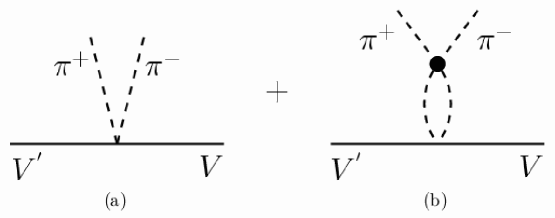
FIG. 1: Diagrams of the vertex $V^{{}^{\prime}}V\pi^{+}\pi^{-}$ without $\pi\pi$ FSI (a) and with $\pi\pi$ FSI (b).

$$\langle\pi^{+}\pi^{-}+\pi^{-}\pi^{+}+\pi^{0}\pi^{0}|t|\pi^{+}\pi^{-}\rangle=2t^{I=0}_{\pi\pi,\pi\pi},$$ (9)

where $t^{I=0}_{\pi\pi,\pi\pi}$ denotes the full $S$ wave $\pi\pi\to\pi\pi$ $t$-matrix in the isospin $I=0$ channel, which is the solution of a set of on-shell coupled channel BSEs [21]. Now, the $t$-matrix for the $V^{{}^{\prime}}\to V\pi^{+}\pi^{-}$ decay can be expressed as

$$t=V_{0}+V_{0S}\cdot G\cdot 2t^{I=0}_{\pi\pi,\pi\pi},$$ (10)

where $V_{0}$ is the amplitude of the tree diagram (a), $V_{0S}$ is the $S$ wave component of $V_{0}$ and $G$ is the two meson loop propagator

$$G=i\int\frac{d^{4}q}{(2\pi)^{4}}\frac{1}{q^{2}-m_{\pi}^{2}+i\varepsilon}\frac{1}{(p^{{}^{\prime}}-p-q)^{2}-m_{\pi}^{2}+i\varepsilon}.$$ (11)

The numerical calculation is done by introducing a three-momentum cutoff $q_{max}$. The value of the cutoff is taken as that used in [21], where the $\pi\pi$ scattering data can be well reproduced up to 1.2 GeV, namely, the $\pi\pi$ FSI in our model is consistent with the $\pi\pi$ scattering data. Moreover, this cutoff is also consistent with the dimensional regularization [22]. The analytic expression of the loop integral in Eq. (11) can be given as

$$G=\frac{1}{8\pi^{2}}\{\sigma\arctan{\frac{1}{\lambda\sigma}}-\ln[\frac{q_{max}}{m_{\pi}}(1+\lambda)]\},$$ (12)

where $\sigma=\sqrt{\frac{4m_{\pi}^{2}}{s}-1}$ and $\lambda=\sqrt{1+\frac{m_{\pi}^{2}}{q^{2}_{max}}}$.

The differential decay width with respect to the $\pi\pi$ invariant mass and $\cos{\theta}^{*}_{\pi}$ reads

$$\frac{d\Gamma}{dm_{\pi\pi}dcos{\theta}^{*}_{\pi}}=\frac{1}{8M^{2}(2\pi)^{3}}\overline{\sum}\sum|t|^{2}|{\bf p_{1}^{*}}||{\bf p_{3}}|$$ (13)

where $\overline{\sum}\sum$ describes the average over initial states and the sum over final states, and ${\bf p_{3}}$ is the 3-momentum of the final vector meson in the lab frame.

3 Results for the $\Psi(2S)\to J/\Psi\pi^{+}\pi^{-}$ decay

In the model, the parameters involved are the coupling constants $g_{1}$, $g_{2}$ and $g_{3}$. The values of the parameters can be determined by fitting the experimental data of the $\Psi(2S)\to J/\Psi\pi^{+}\pi^{-}$ process. It is shown that the resultant $g_{3}$ value is so small that we can safely take $g_{3}=0$. The remaining coupling constants $g_{1}$ and $g_{2}$ are obtained by fitting the total decay rate and the $\pi^{+}\pi^{-}$ invariant mass spectrum simultaneously. The decay data of the $\Psi(2S)\to J/\Psi\pi^{+}\pi^{-}$ process are taken from ref.[34]. These BES data are normalized by using $\Gamma_{\Psi(2S)}=277keV$ and $B(\Psi(2S)\to J/\Psi\pi^{+}\pi^{-})=31.7\%$ [35]. The resultant coupling constants are

$$g_{1}=0.106,~{}~{}~{}~{}~{}~{}g_{2}/g_{1}=-0.319,~{}~{}~{}~{}~{}~{}g_{3}/g_{1}=0.$$ (14)

FIG. 2: $\Psi(2S)\to J/\Psi\pi^{+}\pi^{-}$ decay. (a) $\pi^{+}\pi^{-}$ invariant mass spectrum, and (b) ${\cos\theta_{\pi}^{*}}$ distribution with $\theta_{\pi}^{*}$ being the angle between the moving direction of $\pi^{+}$ in the $\pi^{+}\pi^{-}$ c.m. frame and the moving direction of the $\pi^{+}\pi^{-}$ system in the lab system. The data points are taken from the BES result [34]. The solid curves denote our best fitted results.

Our best fit to the $\pi^{+}\pi^{-}$ invariant mass spectrum and the $\cos\theta_{\pi}^{*}$ distribution are shown in Fig. 2. It is found that the $\pi^{+}\pi^{-}$ invariant mass spectrum is well-fitted, but the theoretical angular distribution is somewhat too flat. Note that in fitting angular distribution, we only consider $\cos\theta_{\pi}^{*}$ from -0.8 to 0.8, because the efficiency correction to the data at large $|\cos\theta_{\pi}^{*}|$ is not accurate enough [34]. The deviation in angular distribution implies that the $D$ wave contribution is somehow too small. In fact, as discussed in Section 2, in our calculation, the $D$ wave FSI is not included. It is also found that the $S$ wave FSI enhances the invariant mass spectrum considerably. It should be noted that due to $P_{2}(\cos\theta_{\pi}^{*})=1/2(\cos^{2}\theta_{\pi}^{*}-1/3)$, integrating over $\cos\theta_{\pi}^{*}$ will result that the $D$ wave contribution is not so important in the invariant mass spectrum. However, in the angular distribution, the $\cos\theta_{\pi}^{*}$-dependence, and consequently the $D$ wave effect, will explicitly show up. Thus, we deem that the deviation in angular distribution may be due to lack of $D$ wave FSI. In fact, it can be confirmed in the following way: In Ref.[34, 11], without FSI, the authors can well-reproduce both the $\pi\pi$ invariant mass spectrum and the angular distribution with $g_{1}=0.30{\pm 0.01}$, $g_{2}/g_{1}$$=-0.35\pm 0.03$ and $g_{3}=0$. However, with the $S$ wave FSI, in the best data fitting to the $\pi\pi$ invariant mass spectrum, the resultant $g_{1}$ is 0.106 which is 3 times less than that in Ref. [11], while $g_{2}/g_{1}$ keeps almost the same value as that in Ref. [11]. This means that the effect of the $S$ wave FSI is so large that $g_{1}$ has to be much smaller to explain the $\pi\pi$ invariant mass spectrum. As a consequence, the $D$ wave component is also greatly reduced. If we naively multiply a factor of 3 to the $D$ wave component, the angular distribution can also be reproduced better. Unfortunately, as mentioned above, the $D$ wave FSI can not be treated properly in the simple ChUT approach [21].

4 The bottomonia $\pi^{+}\pi^{-}$ transitions

Similar to the case of $\Psi(2S)\to J/\Psi\pi^{+}\pi^{-}$, in the $\Upsilon(2S)\to\Upsilon(1S)\pi^{+}\pi^{-}$ or $\Upsilon(3S)\to\Upsilon(2S)\pi^{+}\pi^{-}$ decay, $g_{3}=0$ can be adopted. But for the $\Upsilon(3S)\to\Upsilon(1S)\pi^{+}\pi^{-}$ decay, the $S$ wave FSI is no longer a main contributor, and a finite value of $g_{3}$ is requested. With this consideration, Mannel et al. showed that the resultant values of $g_{2}/g_{1}$ for the $\Upsilon(2S)\to\Upsilon(1S)\pi^{+}\pi^{-}$ and $\Upsilon(3S)\to\Upsilon(2S)\pi^{+}\pi^{-}$ processes are very close, but quite different from that for the $\Upsilon(3S)\to\Upsilon(1S)\pi^{+}\pi^{-}$ process. The latter one is about ten times larger than the former [11]. This is somewhat unnatural. Suffice to say, the pions involved in $\Upsilon(3S)\to\Upsilon(1S)\pi^{+}\pi^{-}$ are somewhat harder than in the other bottomonium transitions, and in principle the values of $g_{2}/g_{1}$ for these processes should not be the same for different dynamical regions. However, in the decay processes considered, the vector mesons involved are all in the $S$ wave state, and the particles involved are in the same mass scale, and the difference among kinematical regions is not too large. Thus we deem that the values of $g_{2}/g_{1}$ for these processes should be very close. To reduce the number of free parameters, we take the same $g_{2}/g_{1}$ value for different $\Upsilon(nS)$ decays.

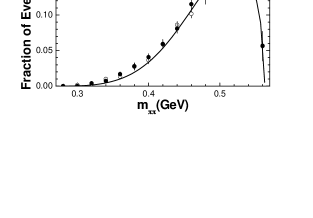
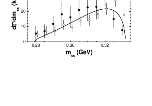
FIG. 3: (a) The $\pi^{+}\pi^{-}$ invariant mass spectrum for the $\Upsilon(2S)\to\Upsilon(1S)\pi^{+}\pi^{-}$ process, (b) the $\cos\theta_{\pi}^{*}$ distribution for the $\Upsilon(2S)\to\Upsilon(1S)\pi^{+}\pi^{-}$ process, and (c) the $\pi^{+}\pi^{-}$ invariant mass spectrum for the $\Upsilon(3S)\to\Upsilon(2S)\pi^{+}\pi^{-}$ process.

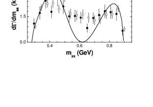
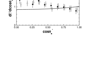
FIG. 4: (a) The $\pi^{+}\pi^{-}$ invariant mass spectrum and (b) the $\cos\theta_{\pi}^{*}$ distribution for the $\Upsilon(3S)\to\Upsilon(1S)\pi^{+}\pi^{-}$ process.

The decay data for $\Upsilon(2S)\to\Upsilon(1S)\pi^{+}\pi^{-}$ are taken from [36] and for $\Upsilon(3S)\to\Upsilon(2S)\pi^{+}\pi^{-}$ and $\Upsilon(3S)\to\Upsilon(1S)\pi^{+}\pi^{-}$ from [1]. To get the physical coupling constants, the data for $\Upsilon(2S)\to\Upsilon(1S)\pi^{+}\pi^{-}$ [36] is normalized by $\Gamma_{\Upsilon(2S)}=43keV$ and $B(\Upsilon(2S)\to\Upsilon(1S)\pi^{+}\pi^{-})=19.2\%$ [35]. Our calculated results are plotted in Figs. 3-4. It is shown that the resultant $\pi\pi$ invariant mass spectra for both $\Upsilon(2S)\to\Upsilon(1S)\pi^{+}\pi^{-}$ and $\Upsilon(3S)\to\Upsilon(2S)\pi^{+}\pi^{-}$ decays agree with the data values, but the angular distribution for the former one is somewhat flat, which might also be due to the same reason discussed in Section 3. On the other hand, there is almost no way to fit the $\pi^{+}\pi^{-}$ invariant mass spectrum and the $\cos\theta_{\pi}^{*}$ distribution of the $\Upsilon(3S)\to\Upsilon(1S)\pi^{+}\pi^{-}$ process simultaneously, even if $g_{2}/g_{1}$ is further released as a free parameter. The resultant parameters are listed in Tab. 1.

TABLE 1: Resultant parameters through data fitting.

Decay	$g_{1}$	$g_{2}/g_{1}$	$g_{3}/g_{1}$
$\Upsilon(2S)\to\Upsilon(1S)\pi^{+}\pi^{-}$	0.0944	-0.230	0
$\Upsilon(3S)\to\Upsilon(2S)\pi^{+}\pi^{-}$	0.768	-0.230	0
$\Upsilon(3S)\to\Upsilon(1S)\pi^{+}\pi^{-}$	0.0123	0.564	-13.602

4.1 Sequential decay mechanism

In order to explain the decay data of the $\Upsilon(3S)\to\Upsilon(1S)\pi^{+}\pi^{-}$ decay, we propose an additional sequential decay mechanism where an intermediate state, called $X$, is introduced. Additional Feynman diagrams for $\Upsilon(nS)\to\Upsilon(mS)\pi^{+}\pi^{-}$ are shown in Fig. 5, where (a) depicts the tree diagram and (b) the diagram including the $\pi\pi$ $S$ wave FSI.

FIG. 5: Diagrams of the sequential $X$ decay mechanism (a) at tree level, and (b) with the $\pi\pi$ FSI.

We adopt a simple $S$ wave coupling for $\Upsilon(nS)\to\pi X$. The quantum numbers of $X$ should be $J^{P}=1^{+}$ and $I=1$. The decay amplitude of Fig. 5(a) can be written as

$$V_{X}^{tree}=g_{nm}\epsilon^{{}^{\prime}}_{\mu}\epsilon^{*}_{\nu}(\frac{-g^{\mu\nu}+p_{X^{+}}^{\mu}p_{X^{+}}^{\nu}/m_{X}^{2}}{p_{X^{+}}^{2}-m_{X}^{2}+im_{X}\Gamma_{X}}+\frac{-g^{\mu\nu}+p_{X^{-}}^{\mu}p_{X^{-}}^{\nu}/m_{X}^{2}}{p_{X^{-}}^{2}-m_{X}^{2}+im_{X}\Gamma_{X}})$$ (15)

where $p_{X^{+}}$ and $p_{X^{-}}$ are the momenta of $X^{+}$ and $X^{-}$ respectively, $g_{nm}$ is an effective coupling constant among $\Upsilon(nS)$, $\Upsilon(mS)$, $\pi^{+}$ and $\pi^{-}$ via an intermediate resonant state $X$. In fact, $g_{nm}$ is the product of two coupling constants $g_{nX}$ and $g_{mX}$ where $g_{kX}(k=n,m)$ denotes the coupling constant for the $\Upsilon(kS)X\pi$ vertex. To further consider the effect of the $\pi\pi$ $S$ wave FSI, the contribution of Fig. 5(b) should be included. In this figure, the three-propagator loop can be expressed as

$$G_{X}^{\mu\nu}=i\int\frac{dq^{4}}{(2\pi)^{4}}\frac{-g^{\mu\nu}+p_{X}^{\mu}p_{X}^{\nu}/m_{X}^{2}}{p_{X}^{2}-m_{X}^{2}+i\varepsilon}\frac{1}{q^{2}-m_{\pi}^{2}+i\varepsilon}\frac{1}{(p^{{}^{\prime}}-p-q)^{2}-m_{\pi}^{2}+i\varepsilon}$$ (16)

where $p_{X}=p^{{}^{\prime}}-q$ is the four-momentum of $X$. The calculation is carried out in the c.m. frame of the $\pi\pi$ system with the same cutoff value used in the two-meson loop calculation. As argued in ref.[20], terms with $\epsilon^{{}^{\prime}}_{\mu}\epsilon^{*}_{\nu}p_{X}^{\mu}p_{X}^{\nu}/m_{X}^{2}$ in Eqs. 15 and 16 can be neglected, because of the expected heavy mass of $X$. Then the total $t$-matrix can finally be written as

$$t=V_{0}+V_{0S}\cdot G\cdot 2t^{I=0}_{\pi\pi,\pi\pi}+V_{X}^{tree}+g_{nm}\epsilon^{{}^{\prime}}_{\mu}\epsilon^{*}_{\nu}G_{X}^{\mu\nu}\cdot 2t^{I=0}_{\pi\pi,\pi\pi}.$$ (17)

4.2 Results for bottomonium $\pi^{+}\pi^{-}$ transitions

In terms of the $t$-matrix in Eq. (17), we calculate the $\pi^{+}\pi^{-}$ invariant mass spectra and the $\cos\theta_{\pi}^{*}$ distributions of the bottomonium $\pi^{+}\pi^{-}$ transitions. Similar to the argument given in the former sections, we take $g_{3}=0$ for the $\Upsilon(2S)\to\Upsilon(1S)\pi^{+}\pi^{-}$ and $\Upsilon(3S)\to\Upsilon(2S)\pi^{+}\pi^{-}$ decays and $g_{3}$ as a free parameter for the $\Upsilon(3S)\to\Upsilon(1S)\pi^{+}\pi^{-}$ process. We also demand the values of $g_{2}/g_{1}$ to be the same for all three decays for reducing the number of free parameters. The values of $g_{1}$ and $g_{2}$ are determined by fitting the experimental decay data [36, 1].

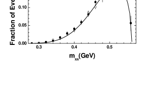
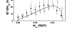
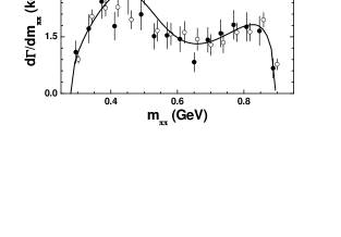
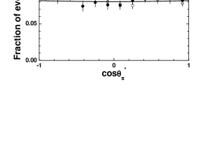
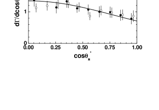
FIG. 6: The $\pi\pi$ invariant mass spectra and the $\cos\theta_{\pi}^{*}$ distributions in the $\Upsilon(nS)\to\Upsilon(mS)\pi^{+}\pi^{-}$ decays.

The calculated results are plotted in Fig. 6. It is shown that not only both the $\pi\pi$ invariant mass spectrum and the $\cos\theta_{\pi}^{*}$ distribution of the $\Upsilon(3S)\to\Upsilon(1S)\pi^{+}\pi^{-}$ process can simultaneously be well explained, but also a consistent description of other bottomonium $\pi^{+}\pi^{-}$ transitions can be obtained. The resultant parameters are tabulated in Tab. 2.

TABLE 2: Resultant parameters in the data fitting. In the first column, $n\to m$ denotes the $\Upsilon(nS)\to\Upsilon(mS)\pi^{+}\pi^{-}$ decay.

Decay	$g_{1}$	$g_{2}/g_{1}$	$g_{3}/g_{1}$	$g_{nm}$(GeV2)	$m_{X}$(GeV)	$\Gamma_{X}$(GeV)
$2\to 1$	0.0886	-0.230	0	-2.316
$3\to 2$	0.769	-0.230	0	-0.00418	10.080	0.655
$3\to 1$	0.00546	-0.230	4.949	4.712

FIG. 7: The contributions from different components to (a) the $\pi^{+}\pi^{-}$ invariant mass spectrum and (b) the $\cos\theta_{\pi}^{*}$ distribution in the $\Upsilon(3S)\to\Upsilon(1S)\pi^{+}\pi^{-}$ decay. The solid curves represent our best fitted results, the dotted, dashed and dash-dotted curves describe the contributions from terms without $X$, with $X$ only and the interference term, respectively. The dash-dot-dotted curves represent the tree level contributions with $X$ only.

To understand thoroughly the roles of different terms in the $\pi^{+}\pi^{-}$ invariant mass spectrum and the $\cos\theta_{\pi}^{\ast}$ distribution of the $\Upsilon(3S)\to\Upsilon(1S)\pi^{+}\pi^{-}$ decay, it is necessary to analyze their individual contributions. The results are shown in Fig. 7. In the figure, the solid curves represent our best fitted results, and the dotted, dashed, and dash-dotted curves describe the contributions from the terms without $X$ and with $X$ only and the interference term respectively, and the dash-dot-dotted curves represent the tree level contributions with $X$ only. The calculated $\pi\pi$ invariant mass spectrum (Fig. 7 (a)) shows that the contribution from $X$ plays a dominant role, the contribution from the terms without $X$ can qualitatively but not quantitatively give the two-peak feature, and the interference term contributes constructively in the smaller $\pi\pi$ invariant mass region but destructively in the larger invariant mass region. The resultant $\cos\theta_{\pi}^{\ast}$ distribution (Fig. 7 (b)) further shows that the contribution from $X$, even in the tree level, produces almost the whole angular distribution structure. Although the scalar meson $\sigma$ dynamically generated by the $S$ wave $\pi\pi$ FSI in ChUT [21] can make a peak around its pole position at about 450 MeV in the $\pi\pi$ invariant mass spectrum, the contribution from the diagrams without $X$ is not dominant due to smaller values of coupling constants. Thus, an additional $D$ wave FSI which provides a flat contribution in the invariant mass region considered will not be an important contributor. These indicate that the intermediate state $X$ is very important in reproducing not only the $\pi^{+}\pi^{-}$ invariant mass spectrum but also the $\cos\theta_{\pi}^{\ast}$ distribution in the $\Upsilon(3S)\to\Upsilon(1S)\pi^{+}\pi^{-}$ decay.

If we further consider the quark structures of the particles involved, the intermediate state should contain $b,~{}\bar{b},~{}q$ and $\bar{q}$. This state might be a tetraquark state, for instance, $b\bar{b}u\bar{d}$, with $J^{P}=1^{+}$ and $I=1$ for $X^{+}$ or a $B\bar{B}$ bound state, for instance, $B^{+}\bar{B}^{0}$, for $X^{+}$.

FIG. 8: Dalitz plot for $\Upsilon(3s)\to\Upsilon(1s)\pi^{+}\pi^{-}$. The mass squared of $\Upsilon(1S)\pi$ system is plotted against the mass squared of the $\pi^{+}\pi^{-}$ system.

It should be mentioned that similar mechanism was also proposed by V.V. Anisovich et al.[20]. In their paper, a trivial $S$ wave coupling was used in the effective vertex $\Upsilon(nS)\Upsilon(mS)\pi\pi$ which is described by Eq. (5) in our model with both $S$ wave and $D$ wave components. With that mechanism, they successfully reproduced the $\pi\pi$ invariant mass spectra of the $\Upsilon(nS)\to\Upsilon(mS)\pi^{+}\pi^{-}$ decays, but did not give reasonable $\cos\theta_{\pi}^{*}$ distributions due to the dominance of the $\pi\pi$ $S$ wave in their model. As a result, the estimated mass of the additional intermediate state is in the range of 10.4-10.8 GeV which is located outside the data area of the Dalitz plot where the data points in the direction of $m_{\Upsilon\pi}$ are located from 9.6 GeV to 10.2 GeV. Thus the effect of the state does not show up in the Dalitz plot.

The mass and width of the intermediate state in our work are different from those in Ref. [20]. We also present the Dalitz plot for the $\Upsilon(3S)\to\Upsilon(1S)\pi^{+}\pi^{-}$ decay in Fig. 8. It is shown that although the estimated mass of $X$ in our model ($M_{X}=10.08$ GeV) is inside the data area in the Dalitz plot, the signal of $X$ in the Dalitz plot is not very clear due to its large width of 0.655 GeV. It does not conflict with the CLEO experiment [36]. Moreover, we would mention that with the typical values, $M_{X}$=10.5 GeV and $\Gamma_{X}$=0.15 GeV given in Ref. [20], we cannot produce a $\cos\theta_{\pi}^{*}$ distribution that is consistent with the experimental data[36].

5 Summary

Starting from an effective Lagrangian and further employing ChUT to include the $\pi\pi$ $S$ wave FSI properly, the $\pi^{+}\pi^{-}$ transitions of heavy quarkonia are intensively studied. In order to consistently explain the $\pi^{+}\pi^{-}$ invariant mass spectra and angular distributions in the mentioned processes simultaneously, especially in the $\Upsilon(3S)\to\Upsilon(1S)\pi^{+}\pi^{-}$ decay process, an additional sequential process, where an intermediate state $X$ is introduced, is further considered in the bottomonium transitions. With such a process included, all the $\pi^{+}\pi^{-}$ transition data can be well-explained, especially the angular distribution of the $\Upsilon(3S)\to\Upsilon(1S)\pi^{+}\pi^{-}$ decay. As a consequence, the newly introduced intermediate state should have quantum numbers of $J^{P}=1^{+}$ and $I=1$, a mass of about 10.08 GeV and a width of about 0.655 GeV. The quark content of the state should be $b\bar{b}q\bar{q}$. It might be a tetraquark state or a $B\bar{B}$ bound state. The detailed inner structure of the state should be carefully studied both theoretically and experimentally.

References

- [1] CLEO Collaboration, F. Butler et al., Phys. Rev. D 49 (1994) 40
- [2] K. Gottfried, Phys. Rev. Lett. 40 (1978) 598
- [3] T.-M. Yan, Phys. Rev. D 22 (1980) 1652
- [4] M. Voloshin and V. Zakharov, Phys. Rev. Lett. 45 (1980) 688
- [5] V. A. Novikov and M. A. Shifman, Z. Phys. C 8 (1981) 43
- [6] Y.-P. Kuang and T.-M. Yan, Phys. Rev. D 24 (1981) 2874
- [7] P. Moxhay, Phys. Rev. D 39 (1989) 3497
- [8] H.-Y. Zhou and Y.-P. Kuang, Phys. Rev. D 44 (1991) 756
- [9] H. J. Lipkin and S. F. Tuan, Phys. Lett. B 206 (1988) 349
- [10] L. Brown and R. Cahn, Phys. Rev. Lett. 35 (1975) 1
- [11] T. Mannel and R. Urech, Z. Phys. C 73 (1997) 541
- [12] M.-L. Yan, Y. Wei and T.-L. Zhuang, Eur. Phys. J. C 7 (1999) 61
- [13] M. Uehara, Prog. Theo. Phys. 109 (2003) 265
- [14] G. Bélanger, T. DeGrand and P. Moxhay, Phys. Rev. D 39 (1989) 257
- [15] S. Chakravarty, S. M. Kim and P. Ko, Phys. Rev. D 48 (1993) 1205
- [16] S. Chakravarty and P. Ko, Phys. Rev. D 48 (1993) 1212
- [17] S. Chakravarty, S. M. Kim and P. Ko, Phys. Rev. D 50 (1994) 389
- [18] A. Gallegos, J. L. Lucio M and J. Pestieau, Phys. Rev. D 69 (2004) 074033
- [19] T. A. Lähde and D. O. Riska, Nucl. Phys. A 707 (2002) 425;
- [20] V. V. Anisovich, D. V. Bugg, A. V. Sarantsev and B. S. Zou, Phys. Rev. D 51 (1995) R4619
- [21] J. A. Oller and E. Oset, Nucl. Phys. A 620 (1997) 438; (Erratum) ibid. 652 (1999) 407
- [22] J. A. Oller, E. Oset and J. R. Peláez, Phys. Rev. Lett. 80 (1998) 3452; Phys. Rev. D 59 (1999) 074001, (Erratum) ibid. 60 (1999) 099906
- [23] J. A. Oller and E. Oset, Nucl. Phys. A 629 (1998) 739
- [24] J. A. Oller and E. Oset, Phys. Rev. D 60 (1999) 074023
- [25] J. A. Oller, Phys. Lett. B 426 (1998) 7
- [26] Ulf-G. Meiner and J. A. Oller, Nucl. Phys. A 679 (2001) 671
- [27] C. Li, E. Oset and M. J. Vicente Vacas, Phys. Rev. C 69 (2004) 015201
- [28] J. E. Palomar, L. Roca, E. Oset and M. J. Vicente Vacas, Nucl. Phys. A 729 (2003) 743
- [29] L. Roca, J. E. Palomar, E. Oset and H. C. Chiang, Nucl. Phys. A 744 (2004) 127
- [30] T. S. H. Lee, J. A. Oller, E. Oset, A. Ramos, Nucl. Phys. A 643 (1998) 402
- [31] J. A. Oller, E. Oset, J. E. Palomar, Phys. Rev. D 63 (2001) 114009
- [32] J. A. Oller, Phys. Rev. D 71 (2005) 054030
- [33] J. A. Oller, E. Oset and A. Ramos, Prog. Part. Nucl. Phys. 45 (2000) 157
- [34] BES Collaboration, J. Z. Bai et al., Phys. Rev. D 62 (2000) 032002
- [35] Particle Data Group, S. Eidelman et al., Phys. Lett. B 592 (2004) 1
- [36] CLEO Collaboration, J. P. Alexander et al., Phys. Rev. D 58 (1998) 052004