Some Results in M-Theory Inspired Phenomenology

Abstract

It is a great pleasure to present this work in honor of Stan Deser whose numerous fundamental contributions to general relativity and supergravity theory have been so important in the development of high energy physics.

We consider string phenomenological models based on 11D Horava-Witten M-theory with 5 branes in the bulk. If the 5-branes cluster close to the distant orbifold plane ($d_{n}\equiv 1-z_{n}\simeq 0.1$) and if the topological charges of the physical plane vanish ($\beta^{(0)}_{i}=0$), then the Witten $\epsilon$ terms (to first order) are correctly small and a qualitative picture of the quark and lepton mass hierarchy arises without significant fine tuning. If right handed neutrinos exist, a possible gravitationally induced cubic holomorphic contribution to the Kahler potential can exist scaled by the 11D Planck mass. These terms give rise to Dirac neutrino masses at the electroweak scale. This mechanism (different from the see-saw mechanism) is seen to account for both the atmospheric and solar neutrino oscillations. The model also gives rise to possible non-universal soft breaking $A$ parameters in the $u$ and $d$ second and third generation quark sector ($A_{2,3}^{(u,d)}$) which naturally can account for the possible (2.4$\sigma$) break down of the Standard Model predictions in the recent B-factory data for the $B\rightarrow\phi K_{s}$ decays.

1 Introduction

With the advent of the “landscape” in M-theory[1] with $10^{100}$(or more!) possible string vacua, it is perhaps more important to try to use phenomenology to help the development of string theory. Thus, for example, the use of the “experimental data” that life exists, i.e. the anthropic principle, has begun to enter cosmology more seriously[2]. In particle theory string phenomenology, one would like to construct a string model that at least semi quantitativelygives rise to Standard Model(SM) physics we know to be true at low energies. This means one wants to do more than just construct a theory that has quarks and leptons arranged in three generations, but one would also like to “explain” at least some of the things the SM can’t explain, such as

• The quark and lepton mass hierarchy e.g. $m_{u}/m_{t}\simeq 10^{-5}$(where $m_{(u,t)}$ are the (u,t) quark masses.

• Supersymmetry(SUSY) soft breaking terms - which one are universal and where non-universalities might occur.

• The origin of neutrino masses

There are of course a huge number of string phenomenology models. We will try to discuss these things here within Horava-Witten M-theory[3, 4, 5, 6] which offers a framework which can allow some of the pecularities of the SM to emerge naturally.

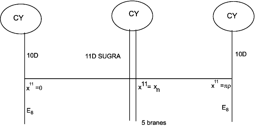
Figure 1: Schemetic picture of H-W M-theory with 5 branes in the bulk. 11D supergravity is in the bulk and $E_{8}$ Yang-Mills fields are on the 10D orbifold planes.

2 Horava-Witten M-theory

We summarize here some of the basic ideas of Horava-Witten (HW) M-theory. In HW theory one considers an 11 dimensional(11D) orbifold, which to lowest order has symmetry $M_{4}\times X\times S_{1}/Z_{2}$ where $M_{4}$ is Minkowski space and $X$ is a Calabi-Yau(CY) 3-fold. In general, supersymmetry allows there to be a set of 5-branes orthogonal to the 11th coordinate x¹¹ wrapped around the CY space with a holomorphic curve.. The orbifold planes are at $x^{11}=0$ (the physical 10D plane) and $x^{11}=\pi\rho$ (the “hidden sector”), shown schematically in Fig.1. To cancel 11D supergravity (SUGRA) anomalies, there must be $E_{8}$ Yang-Mills gauge fields on the orbifold planes, and to make these supersymmetric one must modify the Bianchi identity of the 5-form field strength G of 11D SUGRA to have sources on the orbifold planes and 5-branes:

$$dG_{11\,RSTU} = 4\sqrt{2}\pi(\frac{\kappa}{4\pi})^{2/3}\left[J^{(0)}\delta(x^{11})\right.$$

$$+ \left.J^{N+1}\delta(x^{11}-\pi\rho)+\frac{1}{2}\Sigma_{n=1}^{N}J^{(n)}(\delta(x^{11}-x_{n})+\delta(x^{11}+x_{n}))\right]_{RSTU}.$$

where

$$J^{0} = -\frac{1}{16\pi^{2}}\left(\mathrm{tr}\,F\wedge F-\frac{1}{2}\,\mathrm{tr}\,R\wedge R\right)_{x^{11}=0}$$ (2)

$$J^{N+1} = -\frac{1}{16\pi^{2}}\left(\mathrm{tr}\,F\wedge F-\frac{1}{2}\,\mathrm{tr}\,R\wedge R\right)_{x^{11}=\pi\rho}$$ (3)

$J^{(n)}$, $n=1\ldots N$ are 5-brane sources, $F^{(i)}$, $i=1,2$ are the $E_{8}$ Y-M field strengths, $R$ is the curvature tensor and $\kappa^{-2/9}$ is the 11D Planck mass. The Bianchi identities then imply.

$$\Sigma^{N+1}_{n=0}\beta^{(n)}_{i}=0;\,\,\beta^{n)}_{i}\equiv\int_{C_{i}}J^{(n)},\,n=0,..,N+1.$$ (4)

Finally the quantum theory is gauge invariant provided

$$\lambda^{2}=2\pi(4\pi\kappa)^{2/3}.$$ (5)

where $\lambda$ is the 10D gauge coupling constant.

Thus HW M-theory represents a quantum theory based on the fundamental requirements of anomaly cancelation, Yang-Mills gauge invariance and supergravity invariance. While the $E_{8}$ Yang-Mills invariance guarantees grand unification of the gauge couplings, the additional remarkable thing is that the quantum theory determines the unified (10D) gauge coupling constant $\lambda$ in terms of the (11D) graviational constant $\kappa$ as given in the Eq.(5), and so gauge and gravity are also unified.

Eq.(5) leads to the Witten relations[5] for the GUT coupling constant $\alpha_{G}$ and the Newton constant $G_{N}$

$$\alpha_{G}=\frac{(4\pi\kappa^{2})^{2/3}}{2\mathcal{V}};\,\,\,\,G_{N}=\frac{\kappa^{2}}{16\pi^{2}\mathcal{V}\rho}$$ (6)

where $\mathcal{V}\equiv(M_{G})^{-6}$ is the CY volume. Assuming $M_{G}$ is the GUT mass, $M_{G}\simeq 3\times 10^{16}$ GeV (since experimentally grand unification should occur at the compactification scale) one has ($\alpha_{G}\simeq 1/25$)

$$\kappa^{-2/9}\cong 2M_{G},\,\,(\pi\rho)^{-1}\cong 4.7\times 10^{15}{\rm GeV}$$ (7)

Eq.(7) implies two points. First since the 11 dimensional gravitational mass $\kappa^{-2/9}$ is the fundamental mass of the theory, one sees that $M_{G}$ rather than the Planck mass from $G_{N}$ is the fundamental mass scale. ($M_{pl}$ is a derived 4D quantity from Eq.(6) which is accidentally large.) Second the orbifold length $\pi\rho$ is $O(10)$ times larger than the CY size $M_{G}^{-1}$. Thus Witten discusssed a solution in terms of an expansion in powers of $\kappa^{2/3}$ or more explicitly in powers of the dimensionless parameter

$$\epsilon=(\frac{\kappa}{4\pi})^{2/3}\frac{2\pi^{2}\rho}{\mathcal{V}^{2/3}}$$ (8)

and this has been extensively examined to $O(\epsilon)$. (See[7] and references therein). Actually $\epsilon$ is not small, i.e. $\epsilon\simeq$ 0.9. However for the HW models we will consider $\epsilon$ is multiplied by a small parameter $d_{n}\simeq 0.1$ so that $\epsilon d_{n}$ is indeed small.

Chiral matter arises from expanding the Y-M field strength $F_{\mu{\bar{b}}}$ ($\mu$=0, 1, 2, 3 is in Minkowski space and $b$, ${\bar{b}}$ in CY space) in CY (0,1) harmonic functions $u_{I{\bar{b}}}$:

$$F_{\mu\bar{b}}=\sqrt{2\pi\alpha_{G}}\Sigma_{I}u_{Ib}T_{x}D_{\mu}C^{I}(x)$$ (9)

Here $C^{I}(x)$ are the chiral fields, $I$ is the family index, $T_{x}$ is a group generator. (Thus gauge and chiral matter are also unified.) The quantities needed to construct a phenomenological model to $O(\epsilon)$ (following the analysis of [7]) are the gauge function on the physical orbifold plane

$$f^{(1)}=S+\epsilon T^{i}\left(\beta^{(0)}_{i}+\sum^{N}_{n=1}(1-z_{n})^{2}\beta^{(n)}_{i}\right),$$ (10)

the matter Kahler metric ($K=Z_{IJ}\bar{C^{I}}C^{J}$)

$$Z_{IJ}=e^{-K_{T}/3}\left[G_{IJ}-\frac{\epsilon}{2V}{\Gamma}^{i}_{IJ}(\sum^{N}_{n=1}(1-z_{n})^{2}\beta^{(n)}_{i}+\beta^{(0)}_{i})\right]$$ (11)

and the Yukawa coupling constants

$$Y_{IJK}=2\sqrt{2\pi\alpha_{G}}\lambda_{IJK}\int_{X}\Omega\wedge u_{I}\wedge u_{J}\wedge u_{K}$$ (12)

Here $V=ReS$ is the CY volume modulus, $Rb_{i}\equiv ReT_{i}$ (R is the orbifold modulus),

$$G_{IJ}(a^{i};R)=\frac{1}{{\mathcal{V}}}\int_{X}\sqrt{g}g^{a\bar{b}}u_{Ia}u_{J\bar{b}}$$ (13)

$\Omega$ is the covariantly constant (0,3) form, $z_{n}=x_{n}/{\pi\rho}$ are the positions of the 5-branes and $X$ is the CY space. (Explicit forms for $K_{T}$ and $\Gamma^{i}_{IJ}$ can be[6] found in [7].) Thus $f^{(1)}$ and $Z_{IJ}$ contain a zeroth order piece and an $\epsilon$ correction. Supersymmetry is broken by the Horava mechanism [6] of a condensate on the distant orbifold plane with superpotential.

$$W=hexp[-\frac{6\pi}{b\alpha_{G}}(S+\epsilon T^{i}[-\beta^{(0)}_{i}+\sum^{N}_{n=1}(z_{n}^{2}-1)\beta^{(n)}_{i}]),$$ (14)

where $h\simeq\alpha_{G}/\mathcal{V}$ and $b$=90 (for the $E_{8}$ gauge group on the distant brane).

3 Quark and Lepton Masses

In conventional SUGRA GUT models, one assumes a complicated Yukawa matrix at $M_{G}$ and calculates the masses and CKM matrix at the electroweak scale. Thus for example, a u-quark Yukawa matrix at $M_{G}$ which accounts approximately for the low energy observed electroweak data is given in Fig.2[8].  

$$Y_{U}=\left(\begin{array}[]{ccc}0&\sqrt{2}\lambda^{6}&0\cr\sqrt{2}\lambda^{6}&\sqrt{3}\lambda^{4}&\lambda^{2}\cr 0&\lambda^{2}&1\end{array}\right).$$

Fig.2. The u-quark Yuakawa matrix at $M_{G}$, where $\lambda=0.2$ is the Wolfenstein parameter. 

However, $\lambda^{6}\simeq 10^{-5}$ is needed to obtain $m_{u}/m_{t}\simeq 10^{-5}$ at the electroweak scale, so that the quark mass hierarcy is not explained. In HW theory, the Yukawa matrices are integrals over the CY space, Eq.(12), with no reason to assume that some components should be anomalously small. However, this is not necessarily the case for the Kahler metric for Eq.(11). $Z_{IJ}$ is given there in an expansion in $\epsilon$. As mentioned above, $\epsilon$ is not too small ($\epsilon\simeq 0.9$) making the validity of the expansion in doubt. However, if it were possible to have a CY manifold where $\beta^{(0)}_{i}$=0, then what actually appears in Eqs.(10) and (11) are the combinations

$$\epsilon d_{n}^{2},\,\,\,\epsilon d_{n};\,\,d_{n}\equiv 1-z_{n}$$ (15)

which would be small if $d_{n}\simeq 0.1$. Thus the $\epsilon$ expension would be reasonable (at least in first order) if the 5-branes in Fig.1 all cluster near the distant orbifold plane $x^{11}=\pi\rho$ and the topological parameters $\beta^{(0)}_{i}$ vanish. We will see below that this structure needed for convergence of the $\epsilon$ expansion naturally gives rise to the quark and lepton mass hierarchy.

However, the condition $\beta^{(0)}_{i}$=0 is highly non trivial, and it is possible to show this is impossible for an elliptically fibered CY manifold[9]. This no-go theorem can be evaded, however using a torus fibered CY (with two sections) and one can show that a three generation model with $\beta^{(0)}_{i}$=0 and SU(5) symmetry satisfying all topological constraints exists provided one uses a del Pezzo base $dP_{7}$[10]. (More recently a similar result with SO(10) symmetry has been obtained [11]) The torus fibration also allows for a Wilson line breaking of the $SU(5)$[or $SO(10)$] symmetry at $M_{G}$ to the Standard Model, giving rise to the phenomenologically desired grand unified supergravity GUT model below $M_{G}$.

In the following, we will treat $q\equiv(u_{L},\,u_{R},\,d_{L})$ together [as in SU(5)], and $d_{R}$ seperately. The non-zero elements of $G_{IJ}$ are a priori expected to be $O(1)$. A quark mass spectrum which is qualitatively right can emerge if we assume that the $G_{IJ}$ contributions to $Z_{IJ}$ contribute to all generations for the $d_{R}$ states but only to the first two generations for the $q$ states. The general form then for $Z^{q}$ is shown in Fig.3. The contributions involving the third generations of $Z^{q}$ must be small since $d_{n}$ must be small for the Witten expansion to converge.  

$$Z^{q}=\left(\begin{array}[]{ccc}O(1)&O(1)&O(d_{n}^{2})\cr O(1)&O(1)&O(d_{n}^{2})\cr O(d_{n}^{2})&O(d_{n}^{2})&O(d_{n}^{2})\end{array}\right).$$

Fig.3. The qualitative form of the Kahler matrix $Z^{q}$ for $q\equiv(u_{L},\,u_{R},\,d_{L})$ where $d_{n}\equiv 1-z_{n}\simeq 0.1$ 

The superpotential for the chiral matter fields has the form

$$W_{Y}=e^{\frac{1}{2}K}\frac{1}{3}Y_{IJK}C^{I}C^{J}C^{K}$$ (16)

where $Y_{IJK}$ is given in Eq.(12). For example the $q_{L}u_{R}H_{2}$ coupling [$q_{L}=(u_{L},d_{L})$] (which at the electroweak scale gives rise to the u-quark mass) is

$$W_{Y}=\frac{1}{4R^{3/2}V^{1/2}}(Y^{(u)}q_{L}H_{2}u_{R});\,V\equiv r^{6}.$$ (17)

where we parametrize $V$ by $r^{6}$. To obtain the canonical form, one must reduce $Z_{IJ}$ to a unit matrix. Thus the canonical matter variables are

$$C^{I^{\prime}}={\frac{1}{\sqrt{f_{T}}}}(US)_{IJ}{C^{J}}^{\prime};\,\,f_{T}=e^{-K_{T}/3}$$ (18)

where $U$ diagonalizes $Z_{IJ}$ and $S$ reduces it to a unit matrix

$${\rm diag}S=(\lambda_{1}^{-1/2},\,\lambda_{2}^{-1/2},\,\lambda_{3}^{-1/2}).$$ (19)

Here $\lambda_{i}^{(u,d)}$ are the eigenvalues of $Z_{IJ}$. In terms of canonical variables then, $W_{Y}=u_{L}^{\prime}\lambda^{(u)}u_{R}^{\prime}H_{2}^{\prime}$ where

$$\lambda^{(u)}_{IJ}=\frac{1}{8\sqrt{2}}\frac{1}{R^{3}V^{1/2}}\frac{1}{\sqrt{G_{H_{2}}}}(S^{u}{\tilde{U}^{u}}Y^{u}U^{u}S^{u})_{IJ}$$ (20)

where $H_{2}^{\prime}=\sqrt{G_{H_{2}}}H_{2}$. Since unitary matrices have entries of $O(1)$, the scale of the u-quark masses are qualitatively governed by the eigenvalues of the Kahler matrix i.e.

$$m_{u}:m_{c}:m_{t}=\frac{1}{\lambda^{u}_{1}}:\frac{1}{\lambda^{u}_{2}}:\frac{1}{\lambda^{u}_{3}}$$ (21)

As an example, consider $Z^{u}$ to be

$$Z^{u}=f_{T}\left(\begin{array}[]{ccc}1&1/3&0\cr 1/3&1/8&(2/3)d_{n}^{2}\cr 0&(2/3)d_{n}^{2}&(1/3)d_{n}^{2}\end{array}\right);\,\,d_{n}=1-z_{n}=0.1.$$ (22)

Then

$$\lambda^{u}_{1}=1.12;\,\,\lambda^{u}_{2}=0.0144;\,\,\lambda^{u}_{3}=1.05d_{n}^{4}$$ (23)

and so

$$m_{t}\simeq 100m_{c}\simeq(100)^{2}m_{u}$$ (24)

which is qualitatively correct.

Thus the quark masses hierarchy arises from the effects of the HW 5 branes on the Kahler metric when the 5-branes lie close to the distant orbifold plane. The parameter of smallness in the quark mass matrix is then the geometrical one $d_{n}\equiv 0.1$.

 

$$Z^{u}=f_{T}\left(\begin{array}[]{ccc}1&0.3452&0\cr 0.3452&0.1311&0.006365\cr 0&0.006365&0.00344\end{array}\right);\,\,\,Z^{d}=f_{T}\left(\begin{array}[]{ccc}1&0.496&0\cr 0.496&0.564&0.435\cr 0&0.435&0.729\end{array}\right);$$ (31)

$$Z^{l}=f_{T}\left(\begin{array}[]{ccc}1&-0.547&0\cr-0.547&0.432&0.025\cr 0&0.025&0.09\end{array}\right);\,\,\,Z^{e}=f_{T}\left(\begin{array}[]{ccc}1&0.624&0\cr 0.624&0.397&0.00574\cr 0&0.00574&0.004407\end{array}\right).$$ (38)

Fig.4 Kahler matrices $Z^{(u,d,l,e)}_{IJ}$ and Yukawa matrices $Y^{(u,d,e)}$ for $\tan\beta$=40.

 

 

Quantity	Theoretical Value	Experimental Value
$m_{t}$(pole)	175.2	$174.3\pm 5.1$
$m_{c}$($m_{c}$)	1.27	1.0-1.4
$m_{u}$(1 GeV)	0.00326	0.002-0.006
$m_{b}$($m_{b}$)	4.21	4.0-4.5
$m_{s}$(1 GeV)	0.086	0.108-0.209
$m_{d}$(1 GeV)	0.00627	0.006-0.012
$m_{\tau}$	1.78	1.777
$m_{\mu}$	0.1054	0.1056
$m_{e}$	0.000512	0.000511
$|V_{us}|$	0.221	$0.2210\pm 0.0023$
$|V_{cb}|$	0.042	0.0415$\pm$0.0011
$|V_{ub}|$	$4.96\times 10^{-3}$	$3.80^{+0.24}_{-0.13}\pm 0.45\times 10^{-3}$
$|V_{td}|$	$6\times 10^{-3}$	$9.2\pm 1.4\pm 0.5\times 10^{-3}$
$\sin 2\beta$	0.803	$0.731\pm 0.056$ [15]

Fig. 5. Quarks and leptons masses and CKM matrix elements obtained from the model of Fig.4[12]. Masses are in GeV. Experimental values for lepton and quark masses are from [13] and CKM entries from [14] unless otherwise noted. The only mass input in the second column is $m_{t}$(pole) which sets the scale of all other masses.

 

A similar analysis holds for d-quarks and charged leptons, and a semi-quantitative picture of their mass ratios can also be achieved naturally using only $d_{n}=0.1$. Of course, to precisely get the quark and lepton masses, one must accurately chose $Z^{u,d,e}$, $Y^{u,d,e}$ and one can check that this is possible. Thus Fig.4, in accord with the general HW assumptions stated above, gives rise to the table in Fig.5 for the quark, lepton and CKM elements[12]. Fig.4 determines all the mass ratios and CKM elements and the absolute values of all quark and lepton masses are then obtained by putting in only one mass, i.e. $m_{t}(pole)=175.2$ GeV. The actual value of $m_{t}$ can be related to the CY moduli parameters $R$ and $r$. Thus using Eqs.(17) and (20) for the t-quark gives the relation (for $m_{t}=175$ GeV),

$$Rr(G_{H_{2}})^{1/2}=6.82;\,\,m_{t}=175{\rm GeV}$$ (39)

which is a reasonable condition one might expect to hold for the moduli of the physical CY manifold.

4 Neutrino Masses

The low energy Standard Model does not allow for neutrino masses. The conventional way of introducing neutrino masses is to assume that they arise from GUT scale physics by the see-saw mechanism. Here one assumes the existence of right-handed neutrinos $\nu_{R}$ which develop a GUT size Majorana mass (M) as well as an electroweak scale size Dirac mass (m) with the physical left-handed neutrinos $\nu_{L}$. Eliminating the heavy $\nu_{R}$ fields, one is left with Majorana masses for $\nu_{L}$ of size $m^{2}/M$, which is the size observed experimentally.

The Horava-Witten model offers an alternate possibility for neutrino masses arising from the Kahler potential[12]. Along with the quadratic matter Kahler potential discussed in Sec.3, the Kahler potential can in principle have gravitationally induced cubic terms which would be scaled on dimensional grounds by $1/\kappa_{11}\simeq M_{G}$ (the 11D Planck mass). In general these terms are negligible. An exception arises if there are holomorphic terms involving the $\nu_{R}$ neutrinos. The only gauge invariant holomorphic cubic terms involving $\nu_{R}$ is

$$K_{\nu}=\kappa_{11}Y^{(\nu)}l_{L}H_{2}\nu_{R}$$ (40)

where $l_{L}=(\nu_{L},\,e_{L})$ and $Y^{(\nu)}$ is a neutrino Yukawa matrix. (The possibility of forming this structure is the unique feature of the SUSY SM that $l_{L}$ and $H_{2}$ poseess the same $SU(2)_{L}$ quantum numbers.) By a Kahler transformation one can move this term into the superpotential,

$$K \rightarrow K-K_{\nu},$$

$$W \rightarrow e^{\kappa_{4}^{\;2}K_{\nu}}W=W+\kappa_{4}^{\;2}K_{\nu}W+\cdots$$ (41)

where $1/\kappa_{4}$ is the 4D Planck mass. When supersymmetry breaks, one has the additional superpotential term at $M_{G}$ of

$$W^{\nu}=\left\langle W\right\rangle\frac{\kappa_{4}^{\;2}}{M_{G}}Y^{(\nu)}l_{L}H_{2}\nu_{R}$$ (42)

which leads to Dirac masses at the electroweak scale when $H_{2}$ grows a VEV.

To find the size of the neutrino masses, one must proceed as in the squark and lepton case transforming to canonical fields. $W^{\nu}$ becomes

$$W^{\nu}=\nu_{L}^{\prime}\lambda^{(\nu)}\nu_{R}^{\prime}H_{2}^{\prime}$$ (43)

where

$$\lambda^{(\nu)}_{IJ}=\frac{1}{\sqrt{2}}\frac{1}{R^{3/2}}\frac{1}{\sqrt{G_{H_{2}}}}\frac{\kappa_{4}^{2}\left\langle W\right\rangle}{M_{G}}(S^{(l)}{U^{(l)}}Y^{(\nu)}U^{(\nu)}S^{(\nu)})_{IJ}$$ (44)

Here $S^{(l)}U^{(l)}$ diagonalizes the charge lepton Kahler matrix (and was determined in Sec.3 to obtain the correct lepton masses) while $U^{(\nu)}S^{(\nu)}$ diagonalize the $\nu_{R}$ Kahler matrix $Z^{\nu_{R}}$. As an example we consider $\tan\beta=40$ with $Z^{\nu_{R}}$ and $Y^{\nu}$ of Fig.6 [12] which has the 5-brane induced structure as in $Z^{q}$.  

$$Z^{\nu_{R}}=\left(\begin{array}[]{ccc}1&-0.465&0\cr-0.465&0.3105&2.54d_{n}^{2}\cr 0&2.54d_{n}^{2}&2.7d_{n}^{2}\end{array}\right).$$

$$diagY_{\nu}=\left(4,\,0.4,\,4\right).$$

Fig.6. $Z^{\nu_{R}}$ and $Y^{\nu}$ for the case $\tan\beta=40$. As in the quark lepton sector $d_{n}=0.1$.  Using the renormalization group equations(RGE), one finds at the electroweak scale that $U_{e3}$ is small

$$|U_{e3}|=0.005$$ (45)

and hence the solar($S$) neutrino oscillations are governed by $\Delta m_{21}^{2}$and the atmospheric(A) oscillations by $\Delta m_{32}^{2}$. Thus for the solar oscillations we find[12]

$$\Delta m_{21}^{2}=5.5\times 10^{-5}\,\,\rm{eV}^{2};\,\,\tan^{2}\theta_{12}=0.42.$$ (46)

in accord with the KAMLAND data[17]

$$5.6\times 10^{-5}\leq\Delta m_{S}^{2}/\rm{eV}^{2}\leq 8.9\times 10^{-5}$$ (47)

and for the atmospheric oscillation

$$\Delta m_{32}^{2}=2.7\times 10^{-3}\,\,\rm{eV}^{2};\,\,\tan^{2}\theta_{23}=0.93.$$ (48)

in accord with the SuperKamiokande and K2K large mixing angle solution[18]

$$0.85\leq\sin^{2}2\theta_{A}\leq 1;\,\,\,\,\,1.4\times 10^{-3}\leq\,\,\Delta m_{A}^{2}/\rm{eV}^{2}\leq 3.8\times 10^{-3}.$$ (49)

The mass scale of the neutrino masses is determined by the front factor of Eq.(44),

$$Q=\frac{\kappa_{4}^{2}\left\langle W\right\rangle}{R^{3/2}\sqrt{G_{H_{2}}}M_{G}}$$ (50)

and the above neutrino masses are obtained by choosing

$$Q=1.072\times 10^{-14}$$ (51)

However, there are theoretical constraints on $Q$, as $\left\langle W\right\rangle$ is related to $m_{3/2}$, and one might ask whether Eq.(51) is a reasonable value for Q. One has that

$$m_{3/2}=\frac{5}{\sqrt{12}}\frac{\kappa_{4}^{2}\left\langle W\right\rangle}{R^{3/2}}$$ (52)

Hence,

$$Q=\frac{\sqrt{12}}{5}\frac{1}{\sqrt{G_{H_{2}}}}\frac{m_{3/2}}{M_{G}}$$ (53)

For $m_{3/2}$=500 GeV, one finds that the choice Eq.(51) (which gives the correct size of neutrino masses) is satisfied by:

$$\sqrt{G_{H_{2}}}=1.077$$ (54)

a reasonable result. Thus the smallness of neutrino masses in the model, i.e. the smallness of $Q$ in Eq.(51), is related to the gauge hierarchy i.e. that $m_{3/2}/M_{G}\simeq 10^{-14}$ in Eq.(53). Using the previous result from the t-quark mass, Eq.(39), one then finds

$$R=\frac{6.74}{r}$$ (55)

relating the orbifold and CY moduli.

However, one can go further, since $\left\langle W\right\rangle$ in Eq.(52) can be obtained from Eq.(14):

$$m_{3/2}=\frac{5}{\sqrt{12}}(\frac{r}{6.74})^{3/2}\kappa_{4}^{2}\frac{\alpha_{G}}{\mathcal{V}}exp[-\frac{6\pi}{b\alpha_{G}}(r^{6}-2\epsilon T_{i}\Sigma d_{n}\beta_{i}^{(n)})]$$ (56)

For $m_{3/2}$=500 GeV, Eq.(56) determines $r$, and using Eq.(55) one finds

$$r\simeq 1.34;\,\,\,R\simeq 4.97\,\,{\rm for\,\,m_{3/2}=500\,GeV,\,\,\tan\beta=40}$$ (57)

Thus the model we have constructed giving rise to the quark, lepton, neutrino mass hierarchies implies that the Calabi-Yau and orbifold moduli posseses reasonable values.

5 CP Violation in B Decays and Non-Universal Soft Breaking

In mSUGRA GUT models, one assumes that universal soft breaking of SUSY occurs at $M_{G}$ so that all scalar particles have a common mass $m_{0}$ at $M_{G}$, and the cubic soft breaking mass $A_{0}$ is common for all Yukawa couplings $Y_{IJK}$ at $M_{G}$. This in general is a good fit to all data with one possible exception. Recent measurements at the B factories (BaBar and Belle) for a class of B decays $B\rightarrow\phi K^{0}_{s}$, $B\rightarrow\phi K^{0}_{L}$ and $B\rightarrow\eta^{\prime}K^{0}$ etc., have indicated a possible breakdown of the Standard Model. These decays are unique in two ways. First the SM tree level contribution is zero and so both the SM and SUSY contributions begin at the first loop level. Since both contributions are a priori of comparable size, these decays are a place where the new physics of SUSY might be experimentally observable. Second, at the quark level, all these decays have the general structure of

$$b\rightarrow s+\bar{s}+s$$ (58)

so we are dealing with a well defined class of processes.

B decays exhibit large CP violation and so the B factories can measure both the CP violating phase $\beta$ as well as the branching ratios. In the SM, CP violation stems from a single source, the phase in the CKM matrix. The CP violating phase $\beta$ in B decays is governed by the CKM phase and in the SM one has $\sin 2\beta\simeq 0.73$. However, SUSY allows for additional CP violating phases which could modify the value of $\sin 2\beta$. Averaged over all the $b\rightarrow s$ decays, BaBar finds a 2.7$\sigma$ deviation of $\sin 2\beta$ from the SM results[19] and Belle a 2.4 $\sigma$ deviation[20]. The decay mode that is most theoretically accessible is $B\rightarrow\phi K^{0}_{S}$. Averaging the BaBar and Belle results for this decay, we find $\sin 2\beta_{\phi K_{s}}=0.18\pm 0.23$ which is $2.4\sigma$ deviation from the SM. In addition, the measured branching ratio for both $B^{0}\rightarrow\phi K^{0}$ and $B^{+}\rightarrow\phi K^{+}$ are large. Thus for the well measured $B^{+}$ decay one has Br$[B^{+}\rightarrow\phi K^{+}]$=$(10.9\pm 1.0)\times 10^{-6}$, while over most of the parameter space the SM expects a branching ratio of $5\times 10^{-6}$, much lower than the experimental result.

While the errors are still quite large (and B decay calculations are very complicated) one might ask how one could account for such effects. It turns out that mSUGRA (with universal soft breaking) gives result almost identical to SM[abh1], so if the above results are borne out by further data, they would imply both a breakdown of the Standard Model and of mSUGRA! For a SUGRA GUT model, then the only way one might account for this data would be by assuming non-universal soft breaking at $M_{G}$. If the soft breaking masses have natural (i.e. electroweak) size, then the only non-universal terms that can account for the B decays data is a non-universal cubic soft breaking $A$ parameter mixing the second and third generations in the $u$ or $d$ quark sectors. Detailed calculations[16] then show that

$$|A_{23}^{u,d}|\simeq A_{0}$$ (59)

can correctly give both the experimental $\sin 2\beta_{\phi K_{s}}$ and the $B\rightarrow\phi K$ branching ratios.

It is interesting that the Horava-Witten model we have been considering produces non-universal $A$ parameters in precisely the $A_{23}^{u,d}$ sector. The effective potential for the $A$ soft breaking term is $V_{A}=A_{IJK}C^{I}C^{J}C^{K}$ or

$$V_{A}=A_{IJK}C^{I^{\prime}}C^{J^{\prime}}C^{K^{\prime}}Q^{I}_{I^{\prime}}Q^{J}_{J^{\prime}}Q^{K}_{K^{\prime}}$$ (60)

where $C^{I^{\prime}}$ ar the canonical chiral fields and $Q=US$ reduces the Kahler metric $Z_{IJ}$ to the unit matrix as discussed in Eqs.(18) and (19) above. The soft breaking parameters $A_{IJK}$ are[7]

$$A_{IJK}=F^{a}[\frac{1}{2}\partial_{a}KY_{IJK}-\Gamma^{N}_{a(I}Y_{JK)N}+\partial_{a}Y_{IJK}]$$ (61)

where

$$F^{a}=\kappa_{4}^{2}e^{\frac{K}{2}}K^{a\bar{b}}(\partial_{\bar{b}}W+W\partial_{\bar{b}}K),$$ (62)

$K_{a\bar{b}}=\partial_{a}\partial_{\bar{b}}K$ and W is the superpotential. The first term of Eq. (47) gives rise to the universal soft breaking with

$$A_{0}=\frac{1}{2}F^{a}\partial_{a}K$$ (63)

while the second and third terms give non-universal corrections mixing the generations. The mixing is significant only between the second and third generations since the S matrix elements of Eq.(19), which enters into Eq. (46) are large then since $\lambda_{2,3}$ are small. One can estimate the expected size for $A_{23}^{u,d}$ and finds qualitatively it is about the right size to account for the B factory data, i.e. Eq.(45)[21]. So it possible that this Horava-Witten model can account for the anomalous B data.

6 Conclusions

With the large number of string vacuua and the large number of different string models one might construct, it is of interest to see if one can find string models that can explain naturally some aspects of the Standard Model that are a priori arbitrary (and unreasonable). String theory offers mechanisms to do this that are not available in field theory GUT models. We have considered here the Horava-Witten M-theory with the assumption that the 5-branes in the bulk cluster near the distant brane ($d_{n}=1-z_{n}\simeq 0.1$) and the topological parameters $\beta^{(0)}_{i}$ of the physical brane vanish. This later condition is non-trivial, but allows a three generation model to exist for a Calabi-Yau compactification with torus fibration with two sections and a del Pezzo $dP_{7}$ base. The parameter $d_{n}\simeq 0.1$ then offers a natural parameter to simultaneously help converge the Witten $\epsilon$ expansion and account for the quark and lepton mass hierarchy without significant fine tuning. Thus in this model, the quark and lepton mass hierarchies arise due to the geometrical structure of the model, i.e. the positions of the 5-branes in the bulk. Similarly, the Kahler potential offers an alternate way of introducing neutrino masses, different from the field theoretic see-saw mechanism. The model is distinguishable from the see-saw mechanism in that it gives rise to Dirac neutrino masses and hence no neutrinoless double beta decay. In addition, it predicts that $U_{e3}$ is small, Eq. (31). One can also see the possible origin of non-universal soft breaking terms.

Models of this type are of course not complete. One can not actually calculate Yukawa couplings as these involve integrals over a Calabi-Yau manifold which in general can not be explicitly carried out. (One can only attempt to qualitatively estimate them) While there has been recent work to stabilize string theory moduli[22, 23, 24], one needs an explicit mechanism for stabilizing the 5-branes close to the distant orbifold plane which would give a fundamental explanation for the phenomenological choice of $d_{n}\simeq 0.1$. What one can hope models of this type can do at present give a suggestion as to the direction of where a good string model might be.

References

- [1] M. R. Douglas, JHEP 0305, 046 (2003).
- [2] S. Weinberg, Phys. Rev. Lett. 59, 2607 (1987).
- [3] P. Horava and E. Witten, Nucl. Phys., B460, 506 (1996).
- [4] P. Horava and E. Witten, Nucl. Phys., B475 94 (1996).
- [5] E. Witten, Nucl. Phys. B471, 135 (1996).
- [6] P. Horava, Phys. Rev. D54, 7561 (1996).
- [7] A. Lukas, B. Ovrut and D. Waldram, JHEP 9904, 009 (1999).
- [8] P. Ramond, R. G. Roberts and G. G. Ross, M. Barranco and J. R. Buchler, Phys. Rev. C34, 1729 (1980).
- [9] A. Lukas and B. Ovrut, hep-th/9908100.
- [10] R. Arnowitt and B. Dutta, Nucl. Phys. B592, 143 (2001).
- [11] A. E. Faraggi and R. S. Garavuso, Nucl. Phys. B B659, 224 (2003).
- [12] R. Arnowitt, B. Dutta and B. Hu Nucl. Phys. B682, 347 (2004).
- [13] K. Hagiwara et al., Phys. Rev. D 66, 010001 (2002).
- [14] K. Schubert, talk given at XXI international symposium on lepton and photon interactions at high energies, Fermilab, Batavia, Illinois USA (2003), http://conferences.fnal.gov/lp2003/program/S6/schubert-s06.pdf.
-
[15]
Heavy Flavor Averaging Group,
http://www.slac.stanford.edu/xorg/hfag/index.html. - [16] R. Arnowitt, B. Dutta and B. Hu Phys. Rev. D68, 075008 (2003).
- [17] Super-Kamiokande Collaboration, hep-ex/0309011.
- [18] G. L. Fogli, E. Lisi, A. Marrone and D. Montanino, Phys. Rev. D67, 093006 (2003).
- [19] S. Passaggio, Recent results from BaBar, talk at PASCOS 04, Aug.20,2004, Northeastern University.
- [20] S. Suzuki, Recent results from Belle, talk at PASCOS 04, Aug.20,2004, Northeastern University.
- [21] R. Arnowitt, B. Dutta and B. Hu, in preparation.
- [22] E. Buchbinder, B. Ovrut, [hep-th/0310112].
- [23] S. Kachru, R. Kallosh, A. Linde, S. Trivedi,Phys. Rev.D68,046005 (2003).
- [24] M. Becker, G. Curio, A. Krause, [hep-th/0403027].