Abstract

$SU(2)_{L}$ doublet Higgs fields are unified with gauge fields in the $U(3)_{s}\times U(3)_{w}$ model of Antoniadis, Benakli and Quirós’ on the orbifold $M^{4}\times(T^{2}/Z_{2})$. The effective potential for the Higgs fields (the Wilson line phases) is evaluated. The electroweak symmetry is dynamically broken to $U(1)_{EM}$ by the Hosotani mechanism. There appear light Higgs particles. There is a phase transition as the moduli parameter of the complex structure of $T^{2}$ is varied.

December 1, 2004 OU-HET 494/2004

Gauge fields and Higgs scalar fields in four dimensions are unified in gauge theory in higher dimensions. In particular, gauge theory defined in spacetime with orbifold extra dimensions has recently attracted much attention in constructing phenomenological models.

The idea of unifying Higgs scalar fields with gauge fields was first put forward by Manton and Fairlie.[2] Manton considered $SU(3)$, $O(5)$ and $G_{2}$ gauge theory on $M^{4}\times S^{2}$, supposing that field strengths on $S^{2}$ are nonvanishing in such a way that gauge symmetry breaks down to the electroweak $SU(2)_{L}\times U(1)_{Y}$. Extra-dimensional components of gauge fields of the broken part of the symmetry are the Weinberg-Salam Higgs fields. Higher energy density resulting from nonvanishing field strengths on $S^{2}$, however, leads to the instability of the background configuration. The stabilization of states with nonvanishing flux by quantum effects has been discussed.[3]

The problem of the instability is more naturally solved by considering gauge theory on non-simply connected space. It was shown [4, 5] that quantum dynamics of Wilson line phases can induce gauge symmetry breaking. In particular it was proposed to identify adjoint Higgs fields in grand unified theory (GUT) with extra-dimensional components of gauge fields, which dynamically induces the symmetry breaking such as $SU(5)\rightarrow SU(3)_{c}\times SU(2)_{L}\times U(1)_{Y}$.

Significant progress along this line has been made recently by constructing gauge theory on orbifolds.[6]-[17] In gauge theory on orbifolds, boundary conditions imposed at fixed points on orbifolds incorporate a new way of gauge symmetry breaking. With this orbifold symmetry breaking some of light modes in the Kaluza-Klein tower expansion of fields are eliminated from the spectrum at low energies so that chiral fermions in four dimensions naturally emerge. Furthermore, GUT on orbifolds can provide an elegant solution to the triplet-doublet mass splitting problem of the Higgs fields [9] and the gauge hierarchy problem.[7] There is an attempt to unify all of the gauge fields, Higgs fields and quarks and leptons as well.[13]

In gauge theory on an orbifold, boundary conditions given at the fixed points of the orbifold play an important role. This advantage, however, also implies indeterminacy in theory, namely the arbitrariness problem of boundary conditions.[15] It is desirable to show how a particular set of boundary conditions is chosen naturally or dynamically.

It has been known that in gauge theory on non-simply connected space, different sets of boundary conditions can be physically equivalent by the Hosotani mechanism.[5] It was shown in ref. [14] that there are equivalence relations among different sets of boundary conditions in gauge theory on orbifolds as well. In each equivalence class of boundary conditions, physics is independent of boundary conditions imposed. The physical symmetry is determined by the dynamics of surviving Wilson line phases. Thus the arbitrariness problem of boundary conditions is partly solved.

Dynamics of Wilson line phases are very important in the gauge-Higgs unification in the electroweak theory.[11, 14] In 2001, Antoniadis, Benakli and Quirós proposed an intriguing model of electroweak interactions.[8] $U(3)_{s}\times U(3)_{w}$ gauge theory is defined on $M^{4}\times(T^{2}/Z_{2})$. In this model the weak gauge symmetry $U(3)_{w}\simeq SU(3)_{w}\times U(1)_{w}$ is broken, by the orbifold boundary conditions, to $SU(2)_{L}\times U(1)_{w^{\prime}}\times U(1)_{w}$. The strong group $U(3)_{s}$ is decomposed as $SU(3)_{c}\times U(1)_{s}$. Quarks and leptons are introduced such that among three $U(1)$ groups only one combination, $U(1)_{Y}$, is free from anomalies, while the gauge fields of the other two $U(1)$’s become massive by the Green-Schwarz mechanism. Thus the surviving symmetry at the orbifold scale is $SU(3)_{c}\times SU(2)_{L}\times U(1)_{Y}$.

An amusing feature of this model is that a part of the extra-dimensional components of $SU(3)_{w}$ gauge fields become $SU(2)_{L}$ doublet Higgs fields in four dimensions. They are massless at the tree level. They may acquire nonvanishing vacuum expectation values at the one loop level, thus breaking the electroweak symmetry to $U(1)_{EM}$. At the same time they acquire nonvanishing masses. These points were left unsettled in the original paper by Antoniadis et al. The purpose of this paper is to evaluate the effective potential for the Higgs fields (the Wilson line phases) and examine the resultant spectrum. We find below that physics depends on the matter content and also the moduli parameter of the complex structure of $T^{2}$. We will observe that light Higgs particles appear.

The model is defined on $M^{4}\times(T^{2}/Z_{2})$. Let $x^{\mu}$ $(\mu=0,\cdots,3)$ and $\vec{y}=(y^{1},y^{2})$ be coordinates of $M^{4}$ and $T^{2}$, respectively. Loop translations along the $y^{a}$ axis is given by $\vec{y}\rightarrow\vec{y}+\vec{l}_{a}$ where $\vec{l}_{1}=(2\pi R_{1},0)$ and $\vec{l}_{2}=(0,2\pi R_{2})$. The metric of $T^{2}$ is given by

$$g_{ij}=\pmatrix{1&\cos\theta\cr\cos\theta&1}~{}~{},$$ (1)

where $\theta$ is the angle between the directions of the $y^{1}$ and $y^{2}$ axes. The orbifold $T^{2}/Z_{2}$ is obtained by the $Z_{2}$ orbifolding, namely identifying $\vec{y}$ with $-\vec{y}$. The $Z_{2}$ orbifolding yields four fixed points on $T^{2}/Z_{2}$; $\vec{z}_{0}=\vec{0}$, $\vec{z}_{1}=\hbox{${1\over 2}$}\vec{l}_{1}$, $\vec{z}_{2}=\hbox{${1\over 2}$}\vec{l}_{2}$, and $\vec{z}_{3}=\hbox{${1\over 2}$}(\vec{l}_{1}+\vec{l}_{2})$.

The Lagrangian density must be single-valued; ${\cal L}(x,\vec{y}+\vec{l}_{a})={\cal L}(x,\vec{y})$ $(a=1,2)$ and ${\cal L}(x,\vec{z}_{j}-\vec{y})={\cal L}(x,\vec{z}_{j}+\vec{y})$ $(j=0,\cdots,3)$. However, this does not imply that fields are single-valued. Instead, it is sufficient for gauge fields, for instance, to satisfy [17]

$$\hskip-28.45274ptA_{M}(x,\vec{y}+\vec{l}_{a})=U_{a}A_{M}(x,\vec{y})\,U_{a}^{\dagger}~{}~{},~{}~{}(a=1,2)$$ (2)

$$\hskip-28.45274pt\pmatrix{A_{\mu}\cr A_{y^{I}}\cr}(x,\vec{z}_{i}-\vec{y})=P_{i}\pmatrix{A_{\mu}\cr-A_{y^{I}}\cr}(x,\vec{z}_{i}+\vec{y})\,P_{i}^{\dagger}~{}~{},~{}~{}(i=0,\cdots,3)$$ (3)

where $U_{a}^{\dagger}=U_{a}^{-1}$ and $P_{i}^{\dagger}=P_{i}=P_{i}^{-1}$. The commutativity of two independent loop translations demands $U_{1}U_{2}=U_{2}U_{1}$. Not all of $U_{a}$ and $P_{i}$ are independent; $U_{a}=P_{0}P_{a}$ and $P_{3}=P_{2}P_{0}P_{1}=P_{1}P_{0}P_{2}$.

Let $g_{s}$ and $g$ be gauge coupling constants for the groups $U(3)_{s}$ and $U(3)_{w}$, respectively. The boundary conditions are given by

$$P_{0}=P_{1}=P_{2}={\bf 1}_{3\times 3}\otimes\pmatrix{-1\cr&-1\cr&&+1\cr}~{}~{}.$$ (4)

Note that $U_{1}=U_{2}={\bf 1}_{3\times 3}\otimes{\bf 1}_{3\times 3}$, that is, gauge fields are periodic on $T^{2}$. With the given boundary conditions $SU(3)_{w}$ symmetry breaks down to $SU(2)_{L}\times U(1)_{w^{\prime}}$ at the classical level. There are zero modes of $A_{y^{I}}$, Wilson line phases, on $T^{2}$. They are

$$A_{y^{I}}={1\over\sqrt{2}}\pmatrix{~{}&{\vphantom{{\displaystyle 1\over\displaystyle 2}}}\Phi_{I}\cr~{}~{}\Phi_{I}^{\dagger}~{}&\cr}\quad(I=1,2)~{}.$$ (5)

$\Phi_{1}$ and $\Phi_{2}$ are $SU(2)_{L}$ doublets. At the tree level the Lagrangian density for the zero-modes of $\Phi_{I}$ is given by

$$\hskip-28.45274pt{\cal L}_{\rm tree}(\Phi_{1},\Phi_{2})=g^{jk}(D^{\mu}\Phi_{j})^{\dagger}(D_{\mu}\Phi_{k})-V_{\rm tree}(\Phi_{1},\Phi_{2})$$ (6)

$$\hskip-28.45274ptV_{\rm tree}={g^{2}\over 2\sin^{2}\theta}\Big{\{}\Phi_{1}^{\dagger}\Phi_{1}\cdot\Phi_{2}^{\dagger}\Phi_{2}+\Phi_{2}^{\dagger}\Phi_{1}\cdot\Phi_{1}^{\dagger}\Phi_{2}-(\Phi_{2}^{\dagger}\Phi_{1})^{2}-(\Phi_{1}^{\dagger}\Phi_{2})^{2}\Big{\}}~{},$$ (7)

which has flat directions for $\Phi_{1}=\gamma\Phi_{2}$ ($\gamma$: real), corresponding to the vanishing field strength $F_{y^{1}y^{2}}=0$. The potential $V_{\rm tree}$ does not have the custodial symmetry.

On $T^{2}/Z_{2}$ fermions satisfy

$$\psi(x,\vec{z}_{j}-\vec{y})=\eta_{j}\,T[P_{j}]\,(i\Gamma^{4}\Gamma^{5})\psi(x,\vec{z}_{j}+\vec{y})~{}~{}~{}~{}~{}\quad(j=0,1,2,3)~{}~{}$$ (8)

Here $T[P_{j}]$ stands for an appropriate representation matrix under the gauge group associated with $P_{j}$. If $\psi$ belongs to the fundamental representation, $T[P_{j}]\,\psi=P_{j}\psi$. $\eta_{j}=\pm 1$ and $\eta_{3}=\eta_{0}\eta_{1}\eta_{2}$. $\{\Gamma^{a};(a=0\sim 5)\}$ are six dimensional $8\times 8$ Dirac’s matrices. Four- and six-dimensional chiral operators are given by $\Gamma^{4c}=i\Gamma^{0}\cdots\Gamma^{3}$ and $\Gamma^{6c}=i\Gamma^{4c}\Gamma^{4}\Gamma^{5}$, respectively.

Quarks and leptons are introduced in such a way that only one combination of three $U(1)$’s remains free from anomaly.[8] They come in as six-dimensional (6D) Weyl fermions. Three families of fermions are introduced as

$$\hskip-28.45274ptL_{1,2,3}=({\bf 1,3})^{+}~{}~{},~{}~{}D^{c}_{1,2,3}=({\bf\bar{3},1})^{+}~{}~{},$$ (9)

$$\hskip-28.45274ptQ_{1}=({\bf 3,\bar{3}})^{+}~{}~{},~{}~{}Q_{2}=({\bf 3,\bar{3}})^{-}~{}~{},~{}~{}Q_{3}=({\bf\bar{3},3})^{-}$$ (10)

where $({\bf n_{s},n_{w}})^{\epsilon}$ stands for a fermion with 6D chirality $\epsilon=\pm$ in the representations ${\bf n_{s}}$ and ${\bf n_{w}}$ of $U(3)_{s}$ and $U(3)_{w}$, respectively. Each 6D Weyl fermion is decomposed into 4D left-handed (L) and right-handed (R) fermions. $L_{1}$ in (10), for instance, consists of $L_{1L}=(\nu_{L},e_{L},\tilde{e}_{L})$ and $L_{1R}=(\tilde{\nu}_{R},\tilde{e}_{R},e_{R})$. Among them $\nu_{L}$, $e_{L}$ and $e_{R}$ have zero modes, whereas $\tilde{\nu}_{R}$, $\tilde{e}_{L}$ and $\tilde{e}_{R}$ do not. Let ${\cal Q}_{c}$, ${\cal Q}_{w}$, and ${\cal Q}_{w^{\prime}}$ be appropriately normalized charges of $U(1)_{c}$, $U(1)_{w}$, and $U(1)_{w^{\prime}}$. It has been shown in ref. [8] that with the assignment (10), the charge ${\cal Q}_{Y}=-\frac{1}{3}{\cal Q}_{c}-\frac{2}{3}{\cal Q}_{w}+\frac{1}{6}{\cal Q}_{w^{\prime}}$ is anomaly free. ${\cal Q}_{Y}$ is the weak hypercharge. The resultant theory at low energies is exactly the standard Weinberg-Salam theory of massless quarks and leptons with two Higgs doublets. The weak hypercharge coupling $g_{Y}$ is given by $g^{-2}_{Y}=3g^{-2}+\frac{2}{3}g_{s}^{-2}$. Should the electroweak symmetry breaking take place, the Weinberg angle is given by

$$\sin^{2}\theta_{w}={1\over~{}4+{\displaystyle 2g^{2}\over\displaystyle 3g^{2}_{s}}~{}}~{}~{}.$$ (11)

which is close to the observed value.

The main question is if the electroweak symmetry breaking takes place at the quantum level through the Hosotani mechanism. The effective potential $V_{\rm eff}$ for $\Phi_{I}$ becomes nontrivial even in the flat directions of the potential $V_{\rm tree}$ in (7). The minimum of $V_{\rm eff}$ can be at nontrivial values of $\Phi_{I}$, the symmetry breaking being induced and the Higgs fields acquiring finite masses.

It is sufficient to evaluate the effective potential for a configuration

$$\sqrt{2}gR_{1}\Phi_{1}=\pmatrix{0\cr a\cr}~{}~{},~{}~{}\sqrt{2}gR_{2}\Phi_{2}=\pmatrix{0\cr b\cr}~{}~{},$$ (12)

where $a$ and $b$ are phase variables with a period 2. Depending on the location of the global minimum of $V_{\rm eff}(a,b)$, the physical symmetry varies. To pin down the physical symmetry, it is most convenient to move to a new gauge, in which $\raise 0.68889pt\hbox{$\langle$}\lower 0.68889pt\hbox{}A_{y^{I}}^{\prime}\,\raise 0.68889pt\hbox{$\rangle$}\lower 0.68889pt\hbox{}=0$, by a gauge transformation

$$\Omega(\vec{y}~{};a,b)=\exp\Bigg{\{}i\bigg{(}{\displaystyle ay^{1}\over\displaystyle 2R_{1}}+{\displaystyle by^{2}\over\displaystyle 2R_{2}}\bigg{)}\lambda^{6}\Bigg{\}}~{}~{}.$$ (13)

Then new parity matrices in (3) become

$$P_{0}^{\prime}=\pmatrix{-1&&\cr&-\tau_{3}},\quad P_{1}^{\prime}=\pmatrix{-1&\cr&-{\rm e}^{i\pi a\tau^{1}}\tau^{3}},\quad P_{2}^{\prime}=\pmatrix{-1&\cr&-{\rm e}^{i\pi b\tau^{1}}\tau^{3}}~{}.$$ (14)

As shown in [17], generators commuting with the new $P_{i}^{\prime}$ $(i=0,1,2)$ span the algebra of the physical symmetry. The physical symmetry is given by

$$\cases{SU(2)_{L}\times U(1)_{Y}&for $(a,b)=(0,0)$,\cr\kern 5.0pt\cr U(1)_{EM}\times U(1)_{Z}&for $(a,b)=(0,1),(1,0),(1,1)$,\cr\kern 5.0pt\cr U(1)_{EM}&otherwise.\cr}$$ (15)

For generic values of $(a,b)$, electroweak symmetry breaking takes place and the Weinberg angle is given by (11).

The evaluation of the effective potential is reduced to finding contributions from a $Z_{2}$-doublet $\phi^{t}=(\phi_{1},\phi_{2})$.[14] When $\phi$ satisfies boundary conditions

$$\phi(x,-\vec{y})=\tau_{3}\phi(x,\vec{y})~{}~{},~{}~{}\phi(x,\vec{y}+\vec{l}_{a})=e^{2\pi i\gamma_{a}\tau_{2}}\phi(x,\vec{y})~{}~{},$$ (16)

its mode expansion is given by

$$\hskip-28.45274pt\phi(x,\vec{y})={1\over\sqrt{2\pi^{2}R_{1}R_{2}\sin\theta}}\sum_{n,m=-\infty}^{\infty}\phi_{nm}(x)\pmatrix{\cos c_{nm}(\vec{y})\cr\sin c_{nm}(\vec{y})\cr}$$ (17)

$$\hskip 0.0ptc_{nm}(\vec{y})={\displaystyle(n+\gamma_{1})y_{1}\over\displaystyle R_{1}}+{\displaystyle(m+\gamma_{2})y_{2}\over\displaystyle R_{2}}~{}~{}.$$ (18)

The Lagrangian density for $\phi$, including the interaction with Wilson line phases $\alpha_{j}$, is given by

$${\cal L}_{1}={\displaystyle 1\over\displaystyle 2}g^{jk}D_{j}\phi_{a}D_{k}\phi_{a}~{}~{},~{}~{}D_{j}\phi_{a}=\partial_{j}\phi_{a}-{\displaystyle\alpha_{j}\over\displaystyle R_{j}}\epsilon_{ab}\phi_{b}~{}~{}.$$ (19)

Inserting (18) into $\int d^{2}y\sqrt{g}\,{\cal L}_{1}$, one obtains the spectrum of $\phi_{nm}(x)$ fields. From the spectrum the contribution of $[\phi_{1},\phi_{2};(\gamma_{1},\gamma_{2}),(\alpha_{1},\alpha_{2})]$ to the 1-loop effective potential is found to be $I[\alpha_{1}+\gamma_{1},\alpha_{2}+\gamma_{2};\cos\theta]$ where [18, 8]

$$\hskip-28.45274ptI[\alpha,\beta;\cos\theta]=-{1\over 16\pi^{9}}\Bigg{\{}\sum_{n=1}^{\infty}{\displaystyle\cos 2\pi n\alpha\over\displaystyle n^{6}R_{1}^{6}}+\sum_{m=1}^{\infty}{\displaystyle\cos 2\pi m\beta\over\displaystyle m^{6}R_{2}^{6}}$$ (20)

$$\hskip 28.45274pt+\sum_{n=1}^{\infty}\sum_{m=1}^{\infty}{\displaystyle\cos 2\pi(n\alpha+m\beta)\over\displaystyle(n^{2}R_{1}^{2}+m^{2}R_{2}^{2}+2nmR_{1}R_{2}\cos\theta)^{3}}$$ (21)

$$\hskip 28.45274pt+\sum_{n=1}^{\infty}\sum_{m=1}^{\infty}{\displaystyle\cos 2\pi(n\alpha-m\beta)\over\displaystyle(n^{2}R_{1}^{2}+m^{2}R_{2}^{2}-2nmR_{1}R_{2}\cos\theta)^{3}}\Bigg{\}}~{}.$$ (22)

One unit of $I$ represents contributions to the effective potential from two physical degrees of freedom. Note that $I[-\alpha,\beta;\cos\theta]=I[\alpha,-\beta;\cos\theta]=I[\alpha,\beta;-\cos\theta]$.

Contributions from $SU(3)_{w}$ gauge fields to the effective potential $V_{\rm eff}(a,b)$ in the background field gauge are given, for each degree of freedom, by $V_{\rm eff}^{\rm g+gh}=-{i\over 2}{\rm tr~{}ln}\,D_{L}D^{L}(A_{y^{I}})$, as both the Ricci tensors and background gauge field strengths vanish.[5] For ghost fields the sign is reversed.

For each spacetime component of gauge fields in the tetrad frame we write $B=\sum_{a=1}^{8}\hbox{${1\over 2}$}B_{a}\lambda_{a}$. The four-dimensional components of gauge fields and ghost fields decompose into the following $Z_{2}$-doublets $[\phi_{1},\phi_{2};(\gamma_{1}.\gamma_{2}),(\alpha_{1}.\alpha_{2})]$;

$$\hskip-28.45274pt[-\hbox{${1\over 2}$}(\sqrt{3}B_{3}+B_{8}),B_{6};(0,0),(0,0)]$$ (23)

$$\hskip-28.45274pt[B_{1},B_{5};(0,0),(\hbox{${1\over 2}$}a,\hbox{${1\over 2}$}b)]$$ (24)

$$\hskip-28.45274pt[B_{2},B_{4};(0,0),(-\hbox{${1\over 2}$}a,-\hbox{${1\over 2}$}b)]$$ (25)

$$\hskip-28.45274pt[-\hbox{${1\over 2}$}(B_{3}-\sqrt{3}B_{8}),B_{7};(0,0),(a,b)]~{}.$$ (26)

Similarly, the extra-dimensional components of gauge fields decompose into

$$\hskip-28.45274pt[B_{6},-\hbox{${1\over 2}$}(\sqrt{3}B_{3}+B_{8});(0,0),(0,0)]$$ (27)

$$\hskip-28.45274pt[B_{5},B_{1};(0,0),(-\hbox{${1\over 2}$}a,-\hbox{${1\over 2}$}b)]$$ (28)

$$\hskip-28.45274pt[B_{4},B_{2};(0,0),(\hbox{${1\over 2}$}a,\hbox{${1\over 2}$}b)]$$ (29)

$$\hskip-28.45274pt[B_{7},-\hbox{${1\over 2}$}(B_{3}-\sqrt{3}B_{8});(0,0),(-a,-b)]~{}.$$ (30)

Summing up all these contributions, one finds

$$V_{\rm eff}(a,b)^{\rm g+gh}=4I(0,0)+8I(\hbox{${1\over 2}$}a,\hbox{${1\over 2}$}b)+4I(a,b)~{}~{}.$$ (31)

Here $I(a,b)=I(a,b;\cos\theta)$.

To find contributions from fermions, one notes that the extra-dimensional part of the Dirac operator is given by $\bar{D}=i\Gamma^{a}{e_{a}}^{j}D_{j}(A_{y^{I}})$ ($a=4,5$, $j=y^{j}$) where the tetrad satisfies $\delta^{ab}{e_{a}}_{j}{e_{b}}_{k}=g_{jk}$ and $D_{j}(A_{y^{I}})$ is a covariant derivative. As $T^{2}$ is flat, spin connections vanish. To evaluate the effective potential $V_{\rm eff}(a,b)$ at one loop, it is sufficient to know the spectrum of $\bar{D}$. As $i\Gamma^{4}\Gamma^{5}\psi$ satisfies the same boundary condition (8) as $\psi$ and $i\Gamma^{4}\Gamma^{5}\bar{D}=-\bar{D}i\Gamma^{4}\Gamma^{5}$, eigenvalues $\lambda(a,b)$ of $\bar{D}\psi=\lambda\psi$ always appear in a pair $(\lambda,-\lambda)$. The exception is for modes with $\lambda=0$ which give irrelevant constant contributions to $V_{\rm eff}(a,b)$. Hence contributions from fermions are summarized as $+\hbox{${1\over 2}$}i{\rm tr\,}(D_{4}+\bar{D})=i{\rm tr\,}(D_{4}^{2}+\bar{D}^{2})$.

As the tetrads are constant and the background $F_{y^{1}y^{2}}=0$, $\bar{D}^{2}=-g^{jk}D_{j}D_{k}$. As in the case of bosons, nontrivial contributions arise from $Z_{2}$ doublets. From $L_{1}$, for instance, one has

$$\hskip-28.45274pt[e_{L},i\tilde{e}_{L};(0,0),(\hbox{${1\over 2}$}a,\hbox{${1\over 2}$}b)]$$ (32)

$$\hskip-28.45274pt[e_{R},-i\tilde{e}_{R};(0,0),(-\hbox{${1\over 2}$}a,-\hbox{${1\over 2}$}b)]~{}~{}.$$ (33)

$\nu_{L}$ and $\tilde{\nu}_{R}$ have no coupling to $a$ and $b$. Similar results are obtained for $L_{j}$ and $Q_{j}$. $D_{j}^{c}$ does not couple to $a$ and $b$. To summarize, three families of fermions give

$$V_{\rm eff}(a,b)^{\rm f}=-3\,\Big{\{}14I(0,0)+16I(\hbox{${1\over 2}$}a,\hbox{${1\over 2}$}b)\Big{\}}~{}~{}.$$ (34)

Adding (31) and (34), one finds

$$V_{\rm eff}(a,b)^{\rm total}=-40I(\hbox{${1\over 2}$}a,\hbox{${1\over 2}$}b)+4I(a,b)$$ (35)

up to a constant.

Given $R_{1}$, $R_{2}$ and $\cos\theta$, the absolute minimum of $V_{\rm eff}(a,b)$ is easily found. First note that in the pure gauge theory $V_{\rm eff}(a,b)^{\rm g+gh}$ in (31) has the minimum at $(a,b)=(0,0)$, i.e. $SU(2)_{L}\times U(1)_{Y}$ symmetry remains unbroken. In the presence of fermions the symmetry is partly broken. For $\cos\theta=0$, the minimum of $V_{\rm eff}(a,b)^{\rm total}$ in (35) is located at $(a,b)=(1,1)$. See fig. 1(a). The symmetry breaks down to $U(1)_{EM}\times U(1)_{Z}$. $Z$ bosons remain massless, which is not what is sought for.

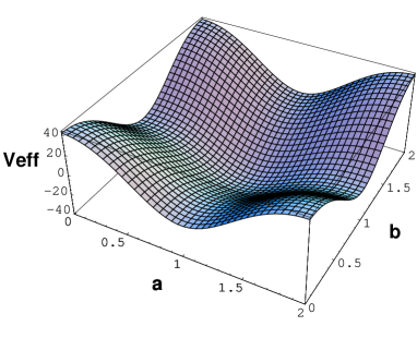
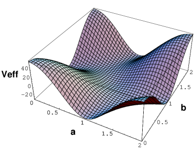
(a)                                                             (b)

Figure 1: $V_{\rm eff}(a,b)$ in (35) for $R_{1}=R_{2}$. (a) $\cos\theta=0$. (b) $\cos\theta=0.5$.

Before presenting models with the electroweak symmetry breaking, we would like to comment that the phase structure critically depends on the value of $\cos\theta$. For $\cos\theta<0.5$, the absolute minimum is located at $(a,b)=(1,1)$. At $\cos\theta=0.5$ with $R_{1}=R_{2}$, there appear three degenerate minima at $(a,b)=(1,1),(0,1),(1,0)$. See fig. 1(b). Notice that the barrier height $V_{\rm B}$ separating the three minima is very small compared with the potential height. For $\cos\theta>0.5$, the absolute minima are given by $(a,b)=(0,1),(1,0)$. Although the physical symmetry in the model leading to $V_{\rm eff}$ in (35) is $U(1)_{EM}\times U(1)_{Z}$ for all values of $\cos\theta$, the spectrum changes at $\cos\theta=0.5$. There is a first-order phase transition there.

Models with the electroweak symmetry breaking are obtained by adding heavy fermions. For each quark/lepton multiplet in (10), which has $(\eta_{0}\eta_{1},\eta_{0}\eta_{2})=(1,1)$ in (8), we introduce three parity partners with $(\eta_{0}\eta_{1},\eta_{0}\eta_{2})=(-1,1),(1,-1),(-1,-1)$. Further we add fermions in the adjoint representation with $(\eta_{0}\eta_{1},\eta_{0}\eta_{2})=(-1,1)$. The total effective potential is, up to a constant,

$$\hskip-28.45274ptV_{\rm eff}(a,b)^{\rm total}=8I(\hbox{${1\over 2}$}a,\hbox{${1\over 2}$}b)+4I(a,b)-N_{Ad}\Big{\{}8I(\hbox{${1\over 2}$}a+\hbox{${1\over 2}$},\hbox{${1\over 2}$}b)+4I(a+\hbox{${1\over 2}$},b)\Big{\}}$$ (36)

$$\hskip 0.0pt-16N_{F}\Big{\{}I(\hbox{${1\over 2}$}a,\hbox{${1\over 2}$}b)+I(\hbox{${1\over 2}$}a+\hbox{${1\over 2}$},\hbox{${1\over 2}$}b)+I(\hbox{${1\over 2}$}a,\hbox{${1\over 2}$}b+\hbox{${1\over 2}$})+I(\hbox{${1\over 2}$}a+\hbox{${1\over 2}$},\hbox{${1\over 2}$}b+\hbox{${1\over 2}$})\Big{\}}~{}.$$ (37)

Here $N_{Ad}$ and $N_{F}$ are the numbers of Weyl fermions in the adjoint representation and of generation of quarks and leptons, respectively. Fermions with $(\eta_{0}\eta_{1},\eta_{0}\eta_{2})\not=(1,1)$ do not have zero modes. For $N_{F}=3$ the spectrum at low energies is the same as in the minimal model leading to (35).

An interesting model is obtained for $N_{Ad}=1$ and $N_{F}=3$. $V_{\rm eff}$ with $N_{Ad}=1$, $N_{F}=3$, $\cos\theta=0$ and $R_{1}=R_{2}$ is displayed in fig. 2. The global minima are located at $(a,b)=(0,\pm 0.269)$. The $SU(2)_{L}\times U(1)_{Y}$ symmetry breaks down to $U(1)_{EM}$. At $\cos\theta=0.1$ the global minima move to $(a,b)=(\pm 0.013,\pm 0.224)$. There is a critical value for $\cos\theta$. At $\cos\theta=0.133\equiv\cos\theta_{c}$, the minima at $(a,b)=(\pm 0.0135,\pm 0.158)$ become degenerate with the minimum at $(a,b)=(0,0)$. For $\cos\theta>\cos\theta_{c}$, the point $(a,b)=(0,0)$ is the global minimum and the symmetry remains unbroken. There is a first-order phase transition at $\cos\theta_{c}$. We note that dynamical electroweak symmetry breaking takes place for $N_{Ad}=0$ and $N_{F}\geq 7$. For instance, the global minima of $V_{\rm eff}$ for $N_{Ad}=0$, $N_{F}=9$, $\cos\theta=0$, and $R_{1}=R_{2}$ are located at $a=\pm b$, $a=\pm 0.320$.

Figure 2: $V_{\rm eff}(a,b)$ in (37) with $N_{Ad}=1$, $N_{F}=3$, $\cos\theta=0$ and $R_{1}=R_{2}$. The minimum is located at $(a,b)=(0,\pm 0.269)$. Dynamical electroweak symmetry breaking takes place.

Let us examine the spectrum of gauge bosons and Higgs particles in the model $N_{Ad}=1$, $N_{F}=3$. The mass of $W$ bosons is given by

$$m_{W}^{2}=\frac{1}{4\sin^{2}\theta}\left(\frac{a_{0}^{2}}{R_{1}^{2}}+\frac{b_{0}^{2}}{R_{2}^{2}}-\frac{2a_{0}b_{0}\cos\theta}{R_{1}R_{2}}\right)~{}.$$ (38)

When $R_{1}=R_{2}=R$, $m_{W}=0.135R^{-1}$ and $0.112R^{-1}$ for $\cos\theta=0$ and $0.1$, respectively. Here $(a_{0},b_{0})$ denotes the location of the global minimum of $V_{\rm eff}$.

The mass of $Z$ bosons is subtle. For $\cos\theta<\cos\theta_{c}$, only photons ($A_{\mu}^{EM}$) remain massless. Let $A_{\mu}^{Y}=A_{\mu}^{Y_{1}}$, $A_{\mu}^{Y_{2}}$ and $A_{\mu}^{Y_{3}}$ be gauge fields associated with the weak hypercharge $Y=Y_{1}$ and the other two $U(1)$ charges $Y_{2}$ and $Y_{3}$. These three gauge fields are related to $A_{\mu}^{w(8)}$ and the two gauge fields associated with $U(1)_{s}$ and $U(1)_{w}$ by an orthogonal transformation. In particular $A_{\mu}^{w(8)}=\sum_{j=1}^{3}\Omega_{1j}A_{\mu}^{Y_{j}}$ where $\Omega\in SO(3)$ and $\sqrt{3}\,\Omega_{11}=\tan\theta_{W}$. The (mass)² matrix in the basis $(A_{\mu}^{w(3)},A_{\mu}^{Y_{j}})$ is given, for $\cos\theta=0$, by

$$\hskip-28.45274ptK=K^{(0)}+K^{(1)}$$ (39)

$$\hskip-14.22636pt=\pmatrix{0\cr&0\cr&&m_{2}^{2}\cr&&&m_{3}^{2}}+m_{W}^{2}\pmatrix{1&-\sqrt{3}\Omega_{1k}\cr\cr-\sqrt{3}\Omega_{1j}&3\Omega_{1j}\Omega_{1k}}~{}.$$ (40)

Here $m_{2}$ and $m_{3}$ are the masses of $A_{\mu}^{Y_{2}}$ and $A_{\mu}^{Y_{3}}$ acquired through the Green-Schwarz mechanism. The second term $K^{(1)}$ arises from the $\hbox{${1\over 2}$}{\rm Tr\,}(F^{w}_{\mu y_{j}})^{2}$ term with nonvanishing $\raise 0.68889pt\hbox{$\langle$}\lower 0.68889pt\hbox{}A^{w}_{y_{j}}\,\raise 0.68889pt\hbox{$\rangle$}\lower 0.68889pt\hbox{}$. We suppose that $m_{2}^{2},m_{3}^{2}\gg m_{W}^{2}$.

One of the eigenstates of $K$ is $A_{\mu}^{EM}$ which has an eigenvector $\vec{v}_{EM}{}^{t}=(\cos\theta_{W},-\sin\theta_{W},0,0)$ with a vanishing eigenvalue. The Weinberg angle is given by (11). The eigenvalue and eigenvector for a $Z$ boson are found in a power series in $m_{W}^{2}/m_{j}^{2}$. One finds

$$m_{Z}^{2}={\displaystyle m_{W}^{2}\over\displaystyle\cos\theta_{W}^{2}}\,\Bigg{\{}1-\bigg{(}\Omega_{12}^{2}{\displaystyle m_{W}^{2}\over\displaystyle m_{2}^{2}}+\Omega_{13}^{2}{\displaystyle m_{W}^{2}\over\displaystyle m_{3}^{2}}\bigg{)}\Bigg{\}}~{}.$$ (41)

Due to the mixing with $A_{\mu}^{Y_{2}}$ and $A_{\mu}^{Y_{3}}$, the $\rho$ parameter ($=m^{2}_{W}/(m^{2}_{Z}\cos^{2}\theta_{W})$) becomes slightly bigger than 1 at the tree level. The correction remains small if the masses generated by the Green-Schwarz mechanism are much larger than $m_{W}$.

A prominent feature of the model is observed in the spectrum of the Higgs particles. In the six-dimensional model there are two Higgs doublets, $\Phi_{1}$ and $\Phi_{2}$. With parametrization

$$\Phi_{j}=\pmatrix{H_{j}\cr 2^{-1/2}(v_{j}+\phi_{j}+i\chi_{j})}$$ (42)

where $(v_{1},v_{2})=(a_{0}/gR_{1},b_{0}/gR_{2})$, the bilinear terms in $V_{\rm tree}$ are given by

$$\hskip-28.45274ptV_{\rm tree}={g^{2}\over 4{\sin^{2}\theta}}(H_{1}^{\dagger},H_{2}^{\dagger})\pmatrix{v_{2}^{2}&-v_{1}v_{2}\cr-v_{1}v_{2}&v_{1}^{2}}\pmatrix{H_{1}\cr H_{2}}$$ (43)

$$\hskip 5.69046pt+{g^{2}\over 2{\sin^{2}\theta}}(\chi_{1},\chi_{2})\pmatrix{v_{2}^{2}&-v_{1}v_{2}\cr-v_{1}v_{2}&v_{1}^{2}}\pmatrix{\chi_{1}\cr\chi_{2}}~{}~{}.$$ (44)

Among charged Higgs fields $(H_{1},H_{2})$, there are two massless modes and two massive modes with a mass $g(v_{1}^{2}+v_{2}^{2})^{1/2}/2\sin\theta$. Neutral CP-odd Higgs fields $(\chi_{1},\chi_{2})$ decompose into one massless mode and one massive mode with a mass $g(v_{1}^{2}+v_{2}^{2})^{1/2}/\sin\theta$. The three massless modes are absorbed by $W$ and $Z$. For $\cos\theta=0$ physical charged Higgs particles and neutral CP-odd Higgs particle have masses $m_{W}$ and $2m_{W}$, respectively.

Neutral CP-even Higgs particles $(\phi_{1},\phi_{2})$ are massless at the tree level, but do acquire finite masses from $V_{\rm eff}^{\rm 1-loop}$. Noting that $a_{j}=a_{j0}+gR_{j}\phi_{j}$, where $(a_{1},a_{2})\equiv(a,b)$, in $V_{\rm eff}(a_{1},a_{2})$, the effective Lagrangian density for the zero modes of $\phi_{j}$ is

$$\hskip-28.45274pt{\cal L}_{\rm eff}={1\over 2}g^{jk}\partial_{\mu}\phi_{j}\partial^{\mu}\phi_{k}-{1\over 2}K^{jk}\phi_{j}\phi_{k}~{}~{},$$ (45)

$$\hskip-28.45274ptK^{jk}=g^{2}R_{j}R_{k}\left.{\displaystyle\partial^{2}V_{\rm eff}\over\displaystyle\partial a_{j}\partial a_{k}}\right|_{\rm min}~{}~{}.$$ (46)

Hence the two eigenvalues of (mass)² are $\hbox{${1\over 2}$}\big{(}A\pm\sqrt{A^{2}-4B\sin^{2}\theta}\big{)}$ where $A=g_{jk}K^{jk}$ and $B=\det K$. In the case $N_{Ad}=1$, $N_{F}=3$, and $R_{1}=R_{2}=R$ in (37), one of the CP-even Higgs particles is much heavier than the other. Let us denote the four-dimensional gauge coupling by $g_{4}^{2}=g^{2}/(2\pi^{2}R^{2}\sin\theta)$. For $\cos\theta=0$, the masses are given by $(0.871,3.26)\times\sqrt{\alpha_{w}}\,m_{W}$ where $\alpha_{w}=g_{4}^{2}/4\pi$. For $\cos\theta=0.1$, they are $(0.799,4.01)\times\sqrt{\alpha_{w}}\,m_{W}$. In the case $N_{Ad}=0$, $N_{F}=9$ and $\cos\theta=0$ in (37), the Higgs masses are given by $(1.039,1.174)\times\sqrt{\alpha_{w}}\,m_{W}$. In the current scheme the mass of the lightest Higgs particle comes out too low.

In the dynamical gauge-Higgs unification scheme in six dimensions, O($m_{W}$) masses of charged and CP-odd neutral Higgs fields are generated from the ${\rm Tr\,}F_{y^{1}y^{2}}^{2}$ term, or $V_{\rm tree}(\Phi)$ in (7). Along the flat directions in $V_{\rm tree}$, there appear light CP-even neutral Higgs fields. Their masses squared are generated at the one loop level and therefore are suppressed by a factor $\alpha_{w}$.

As for the masses of quarks and leptons, the current model yields a mass spectrum which is independent of the generations, and therefore is not realistic. As pointed out in ref. [19], each fermion multiplet can acquire a mass from $Z_{2}$-twists in the boundary conditions on $T^{2}$. By combining this with the VEV of $\Phi_{j}$, it may be possible to produce hierarchy in the mass spectrum.

In this paper we have examined the $U(3)\times U(3)$ model of Antoniadis et al. to find that the electroweak symmetry breaking dynamically takes place through the Hosotani mechanism, provided additional heavy fermions are added. Higgs fields are unified with gauge fields. There appear both neutral and charged Higgs particles at the weak scale. The Weinberg angle comes out about the observed value.

Although it is very encouraging that dynamical electroweak symmetry breaking is implemented in the scheme of the gauge-Higgs unification, there remain several issues to be addressed. First, the Kaluza-Klein mass scale ($1/R$) turns out to be about $10m_{W}$, which is too small. This is a general feature of the models constructed on flat space. The effective potential is minimized at O(1) values of the Wilson line phases (Higgs fields). The Higgsless model on the Randall-Sundrum background[20] and the Hosotani mechanism on the warped spacetime[21] may have a hint for the resolution of this problem. Secondly, the fermion mass spectrum in the model does not distinguish one generation from the others. One of the roles of the Higgs doublets in the Weinberg-Salam theory is to give fermions masses. As the Higgs fields become a part of gauge fields in the gauge-Higgs unification scenario, additional sources for fermion masses need to be introduced. Thirdly the dynamical gauge-Higgs unification scheme generically yields light Higgs particles which may conflict with experimental data. Fourthly it is desirable to extend the model to supersymmetric cases where the Scherk-Schwarz SUSY breaking can induce gauge symmetry breaking.[22] Further, in six dimensions one can introduce bare fermion mass terms as well whose quantum effect on gauge symmetry breaking is of great interest.[23] We hope to come back to these issues in separate publications.

Acknowledgments

This work was supported in part by Scientific Grants from the Ministry of Education and Science, Grant No. 13135215, Grant No. 13640284, and Grant No. 15340078 (Y.H), and by the 21st Century COE Program at Osaka University (K.T.).

References

[1]
[2]
N. Manton, Nucl. Phys. B158 (1979) 141;
D.B. Fairlie, Phys. Lett. B82 (1979) 97;
J. Phys. G5 (1979) L55;
P. Forgacs and N. Manton, Comm. Math. Phys. 72 (1980) 15.
[3]
Y. Hosotani, Phys. Lett. B129 (1984) 193;
Phys. Rev. D29 (1984) 731.
[4]
Y. Hosotani, Phys. Lett. B126 (1983) 309.
[5]
Y. Hosotani, Ann. Phys. (N.Y.)190 (1989) 233.
[6]
A. Pomarol and M. Quiros, Phys. Lett. B438 (1998) 255.
[7]
H. Hatanaka, T. Inami and C.S. Lim,
Mod. Phys. Lett. A13 (1998) 2601;
K. Hasegawa, C.S. Lim and N. Maru, hep-ph/0408028.
[8]
I. Antoniadis, K. Benakli and M. Quiros,
New. J. Phys.3 (2001) 20.
[10]
L. Hall and Y. Nomura, Phys. Rev. D64 (2001) 055003;
Ann. Phys. (N.Y.)306 (2003) 132;
R. Barbieri, L. Hall and Y. Nomura,
Phys. Rev. D66 (2002) 045025;
Nucl. Phys. B624 (2002) 63;
A. Hebecker and J. March-Russell,
Nucl. Phys. B625 (2002) 128;
M. Quiros, hep-ph/0302189.
[11]
M. Kubo, C.S. Lim and H. Yamashita,
Mod. Phys. Lett. A17 (2002) 2249.
[12]
G. Dvali, S. Randjbar-Daemi and R. Tabbash,
Phys. Rev. D65 (2002) 064021;
L.J. Hall, Y. Nomura and D. Smith, Nucl. Phys. B639 (2002) 307;
L. Hall, H. Murayama, and Y. Nomura,
Nucl. Phys. B645 (2002) 85;
G. Burdman and Y. Nomura, Nucl. Phys. B656 (2003) 3;
C. Csaki, C. Grojean and H. Murayama, Phys. Rev. D67 (2003) 085012;
C.A. Scrucca, M. Serone and L. Silverstrini, Nucl. Phys. B669 (2003) 128;
K. Choi et al.,
JHEP0402 (2004) 37;
C.A. Scrucca, M. Serone, L. Silvestrini and A. Wulzer,
JHEP0402 (2004) 49.
[13]
I. Gogoladze, Y. Mimura and S. Nandi,
Phys. Lett. B562 (2003) 307;
Phys. Rev. Lett. 91 (2003) 141801;
Phys. Rev. D69 (2004) 075006.
[14]
N. Haba, M. Harada, Y. Hosotani and Y. Kawamura,
Nucl. Phys. B657 (2003) 169;
Erratum, ibid. B669 (2003) 381;
N. Haba, Y. Hosotani and Y. Kawamura,
Prog. Theoret. Phys. 111 (2004) 265.
[15]
Y. Hosotani, in ”Strong Coupling Gauge Theories and Effective Field
Theories”, ed. M. Harada, Y. Kikukawa and K. Yamawaki (World Scientific
2003), p. 234. (hep-ph/0303066).
[16]
N. Haba, Y. Hosotani, Y. Kawamura and T. Yamashita,
Phys. Rev. D70 (2004) 015010.
[17]
Y. Hosotani, S. Noda and K. Takenaga,
Phys. Rev. D69 (2004) 125014.
[18]
J.E. Hetrick and C.L. Ho, Phys. Rev. D40 (1989) 4085;
C.C. Lee and C.L. Ho, Phys. Rev. D62 (2000) 085021.
[19]
Y. Hosotani, hep-ph/0408012.
[20]
C. Csaki, C. Grojean, L. Pilo, and J. Terning,
Phys. Rev. Lett. 92 (2004) 101802.