B-meson signatures of a
Supersymmetric U(2) flavor model

Abstract

We discuss B-meson signatures of a Supersymmetric U(2) flavor model, with relatively light (electroweak scale masses) third generation right-handed scalars. We impose current $B$ and $K$ meson experimental constraints on such a theory, and obtain expectations for $B_{d}\rightarrow X_{s}\gamma$, $B_{d}\rightarrow X_{s}\,g$, $B_{d}\rightarrow X_{s}\ell^{+}\ell^{-}$, $B_{d}\rightarrow\phi K_{s}$, $B_{s}\bar{B}_{s}$ mixing and the dilepton asymmetry in $B_{s}$. We show that such a theory is compatible with all current data, and furthermore, could reconcile the apparent deviations from Standard Model predictions that have been found in some experiments.

I Introduction

The Standard Model (SM) of high energy physics suffers from the gauge hierarchy problem and the flavor problem. The first is the fine tuning required to maintain a low electroweak mass scale ($M_{EW}$) in the theory, in the presence of a high scale, the Planck Scale ($M_{Pl}$). The second problem is a lack of explanation of the mass hierarchy and mixings of the quarks and leptons.

Supersymmetry (SUSY) eliminates the gauge hierarchy problem by introducing for each SM particle, a new particle with the same mass but different spin. For example, for each SM quark/lepton a new scalar (squark/slepton), and for each SM gauge boson a new fermion (gaugino), is introduced. If SUSY is realized in nature, the fact that we do not see such new particles, we believe, could be because SUSY is spontaneously broken, making the superpartners heavier than the mass ranges probed by experiments. Owing to a lack of understanding of how exactly SUSY is broken, a phenomenologically general Lagrangian, for example, the Minimal Supersymmetric Standard Model (MSSM), is usually considered to compare with data. Various experimental searches have placed constraints on the masses and couplings in the MSSM.

Attempts have been made to address the flavor problem by proposing various flavor symmetries. In a supersymmetric theory, a flavor symmetry in the quark sector might imply a certain structure in the scalar sector, leading to definite predictions for flavor changing neutral current (FCNC) processes on which experiments have placed severe constraints. In the literature, a lot of attention has been devoted toward analyzing the minimal flavor violation (MFV) scenario, in which the scalar flavor structure is aligned with the quark sector so that the two are simultaneously diagonalized. In MFV, the Cabibbo-Kobayashi-Maskawa (CKM) matrix describes the flavor changing interactions in the supersymmetric sector as well, and the only CP violating phase is the one in the CKM matrix. In this work, we do not assume such an alignment, and we will consider non-minimal flavor violation (NMFV), which we treat as a perturbation over the MFV case.

In this paper we wish to explore in what form a supersymmetric extension of the SM, with a U(2) flavor symmetry, could influence K and B physics observables. We thus restrict ourselves to the quark and scalar-quark (squark) sectors. We consider an “effective supersymmetry” Cohen:1996vb framework, with heavy (TeV scale) first two generation squarks, in order to escape neutron electric dipole moment (EDM) constraints. This allows the possibility of having large CP violating phases in the squark sector. We consider a supersymmetric U(2) theory Pomarol:1995xc ; Barbieri:1995uv , impose recent $K$ and $B$ meson experimental constraints and obtain predictions for $B_{d}\rightarrow X_{s}\gamma$, $B_{d}\rightarrow X_{s}\,g$, $B_{d}\rightarrow X_{s}\ell^{+}\ell^{-}$, $B_{d}\rightarrow\phi K_{s}$, $B_{s}\bar{B}_{s}$ mixing and the dilepton asymmetry in $B_{s}$. Though we consider a specific flavor symmetry, namely U(2), our conclusions would hold for any model with a sizable off-diagonal 32 element in the squark mass matrix.

Some $B$ physics consequences in a supersymmetric U(2) theory have been considered in Ref. Barbieri:1995uv . Large $\tan{\beta}$ effects in $B$ decays have been carefully analyzed in Ref. mylgtanb , but for simplicity we will restrict ourselves to the case when $\tan{\beta}$ is not too large. Other work along similar lines, though in more general contexts, have been presented in Refs. Bertolini:1990if ; Hagelin:1992tc ; mygenwk ; Kane:2002sp . In this work we will include all dominant contributions to a particular observable in order to include interference effects between various diagrams. This has not always been done in the literature. We will then study the implications of recent data from the B-factories, including the $b\rightarrow s$ penguin decay mode $B_{d}\rightarrow\phi K_{s}$ which shows a slight deviation from the SM prediction.

The paper is organized as follows: In Section II we specify the supersymmetric U(2) theory we will work with, and the choices we make for the various SUSY and SUSY breaking parameters. In Sections III and IV we consider $\Delta S=2$ (Kaon mixing) and $\Delta B=2$ ($B_{d}\bar{B}_{d}$ and $B_{s}\bar{B}_{s}$ mixing) FCNC process, respectively. In Section V we will consider the implications of such a theory to $\Delta B=1$ FCNC processes, namely $B_{d}\rightarrow X_{s}\gamma$, $B_{d}\rightarrow X_{s}\,g$, $B_{d}\rightarrow X_{s}\ell^{+}\ell^{-}$ and $B_{d}\rightarrow\phi K_{s}$. We conclude in Section VI. We give details of various squark mixings and their diagonalization in Appendix A, and collect loop functions that we will need in Appendix B.

II Supersymmetric U(2)

II.1 The Model

The supersymmetric model that we will discuss is as described in Ref. Barbieri:1995uv , with the first and second generation superfields ($\psi_{a}$, a=1,2) transforming as a U(2) doublet while the third generation superfield ($\psi$) is a singlet. The most general superpotential can be written as :

$${\cal W}=\psi\alpha_{1}H\psi+\frac{\phi^{a}}{M}\psi\alpha_{2}H\psi_{a}+\frac{\phi^{ab}}{M}\psi_{a}\alpha_{3}H\psi_{b}+\frac{\phi^{a}\phi^{b}}{M^{2}}\psi_{a}\alpha_{4}H\psi_{b}+\frac{S^{ab}}{M}\psi_{a}\alpha_{5}H\psi_{b}+\mu H_{u}H_{d},$$ (1)

where $M$ is the cutoff scale below which such an effective description is valid, the $\alpha_{i}$ are O(1) constants, and three new U(2) tensor fields are introduced: $\phi^{a}$ a U(2) doublet, $\phi^{ab}$ a second rank antisymmetric U(2) tensor and $S^{ab}$ a second rank symmetric U(2) tensor. The parameter $\mu$ could be complex and we allow for this possibility. Following Ref. Barbieri:1995uv , we assume that U(2) is broken spontaneously by the vacuum expectation value (VEV) Barbieri:1995uv

$$\left<\phi^{a}\right>=\pmatrix{0\cr V};\ \ \ \left<\phi^{ab}\right>=v\epsilon^{ab};\ \ \ \left<S^{11,12,21}\right>=0,\left<S^{22}\right>=V\ ,$$ (2)

with $V/M\equiv\epsilon\sim 0.02$ and $v/M\equiv\epsilon^{\prime}\sim 0.004$, in order to get the correct quark masses. These VEV’s lead to the quark mass matrix given by (we show only the down quark mass matrix after the $SU(2)_{L}$ is broken by the usual Higgs mechanism)

$${\cal L} \supset -\pmatrix{\bar{d_{R}}&\bar{s_{R}}&\bar{b_{R}}}{\cal M}_{d}\pmatrix{d_{L}\cr s_{L}\cr b_{L}}+{\rm h.c.},$$ (3)

$${\cal M}_{d} = v_{d}\pmatrix{O&-\lambda_{1}\epsilon^{\prime}&O\cr\lambda_{1}\epsilon^{\prime}&\lambda_{2}\epsilon&\lambda_{4}\epsilon\cr O&\lambda_{4}^{\prime}\epsilon&\lambda_{3}},$$

where $v_{d}=\left<h_{d}\right>$ is the VEV of the Higgs field. In ${\cal M}_{d}$, the $\lambda_{i}$’s are O(1) (complex) coefficients, given in terms of the $\alpha_{i}$’s. Ref. Barbieri:1995uv shows that such a pattern of the mass matrix explains the quark masses and CKM elements.

If U(2) is still a good symmetry at the SUSY breaking scale, and broken (spontaneously) only below the SUSY breaking scale, the SUSY breaking terms would have a structure dictated by U(2). For our purposes it is sufficient to consider the down sector squark mass matrices, and they are given as

$${\cal L}\supset-\pmatrix{\tilde{d}_{L}^{*}&\tilde{s}_{L}^{*}&\tilde{b}_{L}^{*}}{\cal M}^{2}_{LL}\pmatrix{\tilde{d}_{L}\cr\tilde{s}_{L}\cr\tilde{b}_{L}}-\pmatrix{\tilde{d}_{R}^{*}&\tilde{s}_{R}^{*}&\tilde{b}_{R}^{*}}{\cal M}^{2}_{RR}\pmatrix{\tilde{d}_{R}\cr\tilde{s}_{R}\cr\tilde{b}_{R}}$$

$$+\left(\pmatrix{\tilde{d}_{R}^{*}&\tilde{s}_{R}^{*}&\tilde{b}_{R}^{*}}{\cal M}^{2}_{RL}\pmatrix{\tilde{d}_{L}\cr\tilde{s}_{L}\cr\tilde{b}_{L}}+{\rm h.c.}\right),$$ (4)

$${\cal M}^{2}_{LL} = {\cal M}_{d}^{\dagger}{\cal M}_{d}+\pmatrix{m_{1}^{2}&i\epsilon^{\prime}m_{5}^{2}&0\cr-i\epsilon^{\prime}m_{5}^{2}&m_{1}^{2}+\epsilon^{2}m_{2}^{2}&\epsilon m_{4}^{2*}\cr 0&\epsilon m_{4}^{2}&m_{3}^{2}}_{LL}+{\rm D-term},$$

$${\cal M}^{2}_{RR} = {\cal M}_{d}{\cal M}_{d}^{\dagger}+\pmatrix{m_{1}^{2}&i\epsilon^{\prime}m_{5}^{2}&0\cr-i\epsilon^{\prime}m_{5}^{2}&m_{1}^{2}+\epsilon^{2}m_{2}^{2}&\epsilon m_{4}^{2*}\cr 0&\epsilon m_{4}^{2}&m_{3}^{2}}_{RR}+{\rm D-term},$$

$${\cal M}^{2}_{RL} = \mu^{*}\tan{\beta}{\cal M}_{d}+v_{d}\pmatrix{O&-A_{1}\epsilon^{\prime}&O\cr A_{1}\epsilon^{\prime}&A_{2}\epsilon&A_{4}\epsilon\cr O&A_{4}^{\prime}\epsilon&A_{3}},$$ (5)

where $m_{i}^{2}$ and $A_{i}$ are determined by the SUSY breaking mechanism. Here $m_{1}^{2},m_{2}^{2},m_{3}^{2}~{}{\rm and}~{}m_{5}^{2}$ are real, while $m_{4}^{2}~{}{\rm and}~{}A_{i}$ could be complex. We will assume that the $A_{i}$ are of order $A$, a common mass scale. The D terms are flavor diagonal, and since we are interested in FCNC processes, we will not write them in detail, but will think of them as included in $m_{1}^{2}$ and $m_{3}^{2}$.

Thus far we have presented the mass matrices in the gauge basis. In the following sections, we will work in the superKM basis in which the quark mass matrix is diagonal, and the quark field rotations that diagonalize the quark mass matrix are applied to the squarks, whose mass matrix would also have been diagonalized in the MFV scheme. Since we will not assume an MFV structure, in the superKM basis, there would be small off-diagonal terms in the squark mass matrix, which we treat as perturbations. The structure of the squark mass matrix in the superKM basis is similar to that in Eq. (5) owing to the smallness of the mixing angles that diagonalize the quark mass matrix.

II.2 SUSY parameters

Lacking specific knowledge about the SUSY breaking mechanism realized in nature, we make some assumptions on the SUSY mass spectrum. Neutron EDM places strong constraints on the CP violating phases and the masses of the first two generations of scalars. To satisfy this and other collider constraints, we consider an “effective SUSY” framework in which the scalars of the first two generations are heavy, suppressing EDM, and allowing for larger CP violating phases. Defining the scalar mass scale, $m_{0}\sim 1~{}{\rm TeV}$, we take all $m_{i}\sim m_{0}$ except for $m_{\tilde{t}_{R},\tilde{b}_{R}}\equiv{m_{3}}_{RR}\sim 100~{}{\rm GeV}$. We take $A\sim m_{0}$, the gaugino mass parameter $M_{2}$ and charged-Higgs masses to be $250~{}{\rm GeV}$ and the gluino mass to be $300~{}{\rm GeV}$. We assume such a spectrum just above the weak scale without specifying what mechanism of SUSY breaking and mediation might actually give rise to it. As we will show later, if realized in nature such a spectrum would lead to enhancements in the processes we are considering here.

The rates of various FCNC processes follow from the mass matrix that we have specified in Eq. (5). We will work in the superKM basis. The interaction vertices in the mass basis are obtained by diagonalizing the mass matrices in Eq. (5), and the perturbative diagonalization to leading order is shown in Appendix. A.

The dominant NMFV SUSY contributions to FCNC processes would be due to the 32 and 23 entries in Eq. (5), since they are the biggest off-diagonal terms. For convenience we define

$$\delta_{32,23}^{RL,RR,LL}\equiv\frac{({\cal M}^{2}_{RL,RR,LL})_{32,23}}{m_{0}^{2}}.$$ (6)

Since we have written down an effective theory and not specified the dynamics of U(2) and SUSY breaking, we can only specify the order of magnitude of $\delta_{32,23}$. To parametrize this uncertainty we write,

$$\delta_{32,23}^{RL}=\frac{v_{d}A\epsilon}{m_{0}^{2}}\,d_{32,23}^{RL},\qquad\delta_{32,23}^{LL,RR}=\frac{\epsilon m_{4}^{2}}{m_{0}^{2}}\,d_{32,23}^{LL,RR}\ ,$$ (7)

where we have denoted the unknown $\mathcal{O}(1)$ coefficients by $d_{32,23}^{LL,RR,RL}$.

$m_{0}$	$1000\$	$\tan{\beta}$	$5\$
${m_{\tilde{b}_{R},\tilde{t}_{R}}}$	$100\$	$\mu$	$200\,e^{i\,2.2}\$
${m_{\tilde{d}_{R},\tilde{s}_{R}}}$	$1000\$	$M_{2}$	$250\$
${m_{\tilde{q}_{L}}}$	$1000\$	$M_{\tilde{g}}$	$300\$
$A$	$1000\$	$m_{H^{\pm}}$	$250\$
$\ d_{32}^{RL}\$	$~{}2\,e^{i\,3.2}\$	$\ d_{32}^{RR}\$	$1.75\,e^{i\,1.6}\$

Table 1: Default SUSY parameters for this work that satisfy all experimental constraints discussed in this paper. All masses are in GeV.

We summarize our choice of the parameters in Table 1. For these values, from Eq. (7), the natural sizes of $\delta_{32,23}$ are given by

$$\delta_{32,23}^{RL}=6.82\times 10^{-4}\,d_{32,23}^{RL}\ ,\qquad\delta_{32,23}^{LL,RR}=0.02\,d_{32}^{LL,RR}\ .$$ (8)

We will find in the rest of this paper that $\delta^{RL}$ induces NMFV $\Delta B=1$ FCNC processes dominantly, while $\delta^{RR,LL}$ induces $\Delta S=2$ and $\Delta B=2$ FCNC processes. Though the $\delta_{32}^{RL}$ and $\delta_{23}^{RL}$ elements have similar magnitudes, the $\delta_{32}^{RL}$ gluino NMFV contribution to $\Delta B=1$ FCNC processes is larger, since we take $\tilde{b}_{R}$ to be much lighter than the other scalars, and the $\delta_{23}^{RL}$ gluino diagrams are relatively suppressed by the heavier $\tilde{b}_{L}$ mass. Therefore, in this work we will include only the dominant $\delta_{32}^{RL}$ contribution. We illustrate this in Fig. 1, where we show the gluino contribution to $B_{d}\rightarrow X_{s}\gamma$ as an example.

Figure 1: Gluino contribution to $B_{d}\rightarrow X_{s}\gamma$. The diagram on the left, proportional to $\delta_{32}^{RL}$, has the lighter scalar $\tilde{b}_{R}$, while the one on the right, proportional to $\delta_{23}^{RL}$, only has heavier scalars and is therefore relatively suppressed.

Similarly, owing to the smaller $\tilde{b}_{R}$ mass, the $\delta_{32,23}^{RR}$ NMFV contribution to $\Delta S=2$ and $\Delta B=2$ FCNC processes is relatively larger compared to the $\delta_{32,23}^{LL}$ contribution. We note here that, from Eq. (62) in Appendix A, the sbottom mixing angle is negligibly small, and therefore, we ignore sbottom mixing effects; stop mixing is not as small and we include its effects.

In the next three sections we will discuss the implication of the U(2) model to $\Delta S=2$, $\Delta B=2$ and $\Delta B=1$ FCNC processes. From this we will see that present experimental data are compatible with the values shown in Table 1, and we will obtain expectations for some measurements that are forthcoming. We will present plots of different FCNC effects by varying a couple of parameters at a time, while keeping all others fixed at the values shown in Table 1.

III $\Delta S=2$ FCNC process

The CP violation parameter $\epsilon_{K}$ due to mixing in the Kaon sector has been measured to be Eidelman:2004wy

$$|\epsilon_{K}|=\left(2.284\pm 0.014\right)\times 10^{-3}\ .$$ (9)

We wish to estimate the new physics contributions to $\epsilon_{K}$ in the scenario that we are considering. Here we note that even though the direct CP violation parameter $\epsilon_{K}^{\prime}/\epsilon_{K}$ has also been measured, large hadronic uncertainties do not permit us to constrain new physics models through this observable.

Kaon mixing is governed by the $\Delta S=2$ effective Hamiltonian

$${\cal H}^{eff}_{\Delta S=2}=\sum_{i=1}^{5}C_{i}Q_{i}+\sum_{i=1}^{3}\tilde{C}_{i}\tilde{Q}_{i}\ ,$$ (10)

where,

$$Q_{1} = \bar{d}_{L}^{\alpha}\gamma_{\mu}s_{L}^{\alpha}\bar{d}_{L}^{\beta}\gamma^{\mu}s_{L}^{\beta}\ ,$$

$$Q_{2} = \bar{d}_{R}^{\alpha}s_{L}^{\alpha}\bar{d}_{R}^{\beta}s_{L}^{\beta}\ ,$$

$$Q_{3} = \bar{d}_{R}^{\alpha}s_{L}^{\beta}\bar{d}_{R}^{\beta}s_{L}^{\alpha}\ ,$$

$$Q_{4} = \bar{d}_{R}^{\alpha}s_{L}^{\alpha}\bar{d}_{L}^{\beta}s_{R}^{\beta}\ ,$$

$$Q_{5} = \bar{d}_{R}^{\alpha}s_{L}^{\beta}\bar{d}_{L}^{\beta}s_{R}^{\alpha}\ .$$ (11)

The operators $\tilde{Q}_{i}$ (i=1,2,3) are obtained by exchanging $L\leftrightarrow R$. In the SM and the new physics model we are considering, the dominant contributions are to $Q_{1}$, as we explain later in this section. The CP violation parameter $\epsilon_{K}$ is then given by (see for example Ref. Branco:1994eb )

$$\epsilon_{K}=e^{i\pi/4}\frac{1}{3\sqrt{2}}\frac{m_{K}B_{K}f_{K}^{2}}{\Delta m_{K}}~{}{\rm Im}\left[C_{1}(m_{K})\right]\ ,$$ (12)

where $B_{K}$ is the Bag parameter and $f_{K}$ is the Kaon decay constant.

In addition to the SM $W$ box diagram contribution to $C_{1}$, in the supersymmetric U(2) theory we are considering, the charged-Higgs and chargino MFV contributions could be sizable. The dominant MFV contributions to $C_{1}$ can be written as

$$C_{1}^{MFV}=C_{1}^{W}+C_{1}^{H}+C_{1}^{\chi}\ ,$$ (13)

which is the sum of the SM $W$, the charged-Higgs, and the chargino contributions, respectively.
SM contribution: The SM $W$ contribution is Buchalla:1995vs

$$C_{1}^{SM}(m_{t})=C_{1}^{W}(m_{t})=\frac{G_{F}^{2}m_{W}^{2}}{4\pi^{2}}~{}~{}\Biggl{\{}\left(V_{td}^{*}V_{ts}\right)^{2}~{}S_{0}(x_{t})$$

$$\Biggl{.}+\left(V_{cd}^{*}V_{cs}\right)^{2}~{}S_{0}(x_{c})+2\left(V_{td}^{*}V_{ts}V_{cd}^{*}V_{cs}\right)~{}S_{0}(x_{t},x_{c})\Biggl{\}}\ ,$$ (14)

where the function $S_{0}$ is given in Appendix B, Eq. (72), and $x_{t}\equiv m_{t}^{2}/m_{W}^{2}$, $x_{c}\equiv m_{c}^{2}/m_{W}^{2}$. The QCD correction due to renormalization group running from $m_{t}$ to $m_{b}$ gives

$$C_{1}^{SM}(m_{K})=C_{1}^{W}(m_{K})=\frac{G_{F}^{2}m_{W}^{2}}{4\pi^{2}}~{}~{}\Biggl{\{}\left(V_{td}^{*}V_{ts}\right)^{2}\eta_{K33}~{}S_{0}(x_{t})$$

$$\Biggl{.}+\left(V_{cd}^{*}V_{cs}\right)^{2}\eta_{K22}~{}S_{0}(x_{c})+2\left(V_{td}^{*}V_{ts}V_{cd}^{*}V_{cs}\right)\eta_{K32}~{}S_{0}(x_{t},x_{c})\Biggl{\}}\ ,$$ (15)

where the $\eta_{K}$ are QCD correction factors given in Eq. (20) below, and $V_{ij}$ are the CKM matrix elements.
Charged-Higgs contribution: Supersymmetric theories require two Higgs doublets to give masses to the up and down type fermions. The Higgs doublets contain the charged-Higgs $H^{\pm}$, and the dominant charged-Higgs-top contribution is Branco:1994eb

$$C_{1}^{H}(m_{t}) = \frac{G_{F}^{2}m_{W}^{2}}{4\pi^{2}}\left(V_{td}^{*}V_{ts}\right)^{2}~{}\left[-F_{V}^{H}\right]\ ,$$ (16)

$$F_{V}^{H} = \frac{1}{4\tan^{4}\beta}x_{t}^{2}~{}Y_{1}(r_{H},r_{H},x_{t},x_{t})+\frac{1}{2\tan^{2}\beta}x_{t}^{2}~{}Y_{1}(1,r_{H},x_{t},x_{t})-\frac{2}{\tan^{2}\beta}x_{t}~{}Y_{2}(1,r_{H},x_{t},x_{t})\ ,$$

where $r_{H}\equiv m_{H}^{2}/m_{W}^{2}$, and the functions $Y_{1}$ and $Y_{2}$ are given in Appendix B, Eq. (73).
Chargino contribution: The dominant chargino-right-handed-stop contribution is Branco:1994eb

$$C_{1}^{\chi}(m_{t}) = \frac{G_{F}^{2}m_{W}^{2}}{4\pi^{2}}\left(V_{td}^{*}V_{ts}\right)^{2}\left[-F_{V}^{\chi}\right]\ ,$$ (17)

$$F_{V}^{\chi} = \frac{1}{4}|\Gamma_{\chi R}^{(i)}|^{2}|\Gamma_{\chi R}^{(j)}|^{2}~{}Y_{1}(r_{\tilde{t}_{2}},r_{\tilde{t}_{2}},s_{i},s_{j})\ ,$$

where $r_{\tilde{t}_{2}}\equiv m_{\tilde{t}_{2}}^{2}/m_{W}^{2}$, $s_{1,2}\equiv m_{\tilde{\chi}_{1,2}}^{2}/m_{W}^{2}$, and the coupling is given by

$$\Gamma_{\chi R}^{(i)}=\sqrt{2}({\cal C}_{R}^{*})_{1i}({\cal C}_{\tilde{t}}^{*})_{12}-\frac{({\cal C}_{R}^{*})_{2i}({\cal C}_{\tilde{t}}^{*})_{22}}{\sin\beta}\frac{m_{t}}{m_{W}}\ ,$$ (18)

with the chargino and stop diagonalization matrices $({\cal C}_{R})$ and $({\cal C}_{\tilde{t}})$ given in Appendix A, Eqs. (57) and (61), respectively . Taking into account renormalization group running, we have

$$C_{1}^{H,\chi}(m_{K})\approx\eta_{K33}~{}C_{1}^{H,\chi}(m_{t})\ .$$ (19)

Gluino contribution: In general, the NMFV gluino contributions induce many operators shown in Eq. (11), but in the model we are considering, these are not significant due to a suppression from the heavy $\tilde{d}$ and $\tilde{s}$ masses, Glashow-Iliopoulos-Maiani (GIM) suppression owing to their approximate degeneracy (split only by $\mathcal{O}(\epsilon^{2})$, cf. Eq. (5)), and the contribution from the relatively light right-handed sbottom being suppressed by its small mixing to the first two generations. Moreover, owing to the structure of the mass matrix, Eq. (5), the gluino contribution is real, and hence does not contribute to $\epsilon_{K}$.

In our numerical analysis, we take the following values for the various parameters Eidelman:2004wy ; Buchalla:1995vs :

$$\eta_{K33} = 0.57\ ,\quad\eta_{K22}=1.38\ ,\quad\eta_{K32}=0.47\ ,$$

$$f_{K} = 0.160~{}{\rm GeV}\ ,\quad 0.6<B_{K}<0.9\ ,$$ (20)

$$m_{K} = 0.497~{}{\rm GeV}\ ,\quad\Delta m_{K}=(3.48\pm 0.01)\times 10^{-15}~{}{\rm GeV}\ ,\quad m_{c}=(1.2\pm 0.2)~{}{\rm GeV}\ .$$

The SM prediction for $\epsilon_{K}$ is in agreement with the experimental data, but it should be noted that there is considerable uncertainty in the lattice computation of the Bag parameter $B_{K}$ (see Eq. (20)). The chargino and charged-Higgs contributions to $C_{1}$ add constructively with the SM contribution. Therefore, if the true value of $B_{K}$ is taken to be closer to the lower limit, we can allow MFV contributions to be up by a factor of 1.2 compared to the SM value; i.e., ${\rm Im}(C_{1}^{MFV})/{\rm Im}(C_{1}^{SM})\lower 3.01385pt\hbox{$\;\stackrel{{\scriptstyle\textstyle<}}{{\sim}}\;$}1.2$. Fig. 2 shows the region of MFV parameter space where this is satisfied. This justifies some of the choices we make in the list shown in Table 1.

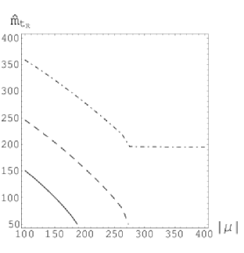
Figure 2: The (dash-dot, dash, solid) curves are (1.05, 1.1, 1.2) contours of ${\rm Im}(C_{1}^{MFV})/{\rm Im}(C_{1}^{SM})$, showing the MFV contributions to Kaon mixing relative to the SM. Parameters not shown on a plot’s axes are fixed as shown in Table 1.

IV $\Delta B=2$ FCNC processes

IV.1 General formalism

We start by discussing in general $B_{q}\bar{B}_{q}$ mixing and later specialize in succession to $B_{d}\bar{B}_{d}$ (q=d) and to $B_{s}\bar{B}_{s}$ (q=s). The $\Delta B=2$ effective Hamiltonian is given by Becirevic:2001jj :

$${\cal H}^{eff}_{\Delta B=2}=\sum_{i=1}^{5}C_{i}Q_{i}+\sum_{i=1}^{3}\tilde{C}_{i}\tilde{Q}_{i}\ ,$$ (21)

where, for $B_{q}$,

$$Q_{1} = \bar{q}_{L}^{\alpha}\gamma_{\mu}b_{L}^{\alpha}\bar{q}_{L}^{\beta}\gamma^{\mu}b_{L}^{\beta}\ ,$$

$$Q_{2} = \bar{q}_{R}^{\alpha}b_{L}^{\alpha}\bar{q}_{R}^{\beta}b_{L}^{\beta}\ ,$$

$$Q_{3} = \bar{q}_{R}^{\alpha}b_{L}^{\beta}\bar{q}_{R}^{\beta}b_{L}^{\alpha}\ ,$$

$$Q_{4} = \bar{q}_{R}^{\alpha}b_{L}^{\alpha}\bar{q}_{L}^{\beta}b_{R}^{\beta}\ ,$$

$$Q_{5} = \bar{q}_{R}^{\alpha}b_{L}^{\beta}\bar{q}_{L}^{\beta}b_{R}^{\alpha}\ .$$ (22)

The operators $\tilde{Q}_{i}$ (i=1,2,3) are obtained by exchanging $L\leftrightarrow R$. The Wilson coefficients $C_{i}$ are run down from the SUSY scale, $M_{S}$, using Becirevic:2001jj

$$C_{r}(m_{b})=\sum_{i}\sum_{s}\left(b_{i}^{(r,s)}+\eta c_{i}^{(r,s)}\right)\eta^{a_{i}}C_{s}(M_{S})$$ (23)

where $\eta\equiv\alpha_{s}(M_{S})/\alpha_{s}(m_{t})$ and the $a_{i}$, $b_{i}$ and $c_{i}$ are constants given in Ref. Becirevic:2001jj .

The matrix elements of the $Q_{i}$ in the vacuum insertion approximation are given by Becirevic:2001jj ; Ko:2002ee .

$$\left<\bar{B}_{q}|Q_{1}(\mu)|B_{q}\right> = \frac{2}{3}m_{B_{q}}^{2}f_{B_{q}}^{2}B_{1}(\mu)\ ,$$

$$\left<\bar{B}_{q}|Q_{2}(\mu)|B_{q}\right> = -\frac{5}{12}\left(\frac{m_{B_{q}}}{m_{b}+m_{q}}\right)^{2}m_{B_{q}}^{2}f_{B_{q}}^{2}B_{2}(\mu)\ ,$$

$$\left<\bar{B}_{q}|Q_{3}(\mu)|B_{q}\right> = \frac{1}{12}\left(\frac{m_{B_{q}}}{m_{b}+m_{q}}\right)^{2}m_{B_{q}}^{2}f_{B_{q}}^{2}B_{3}(\mu)\ ,$$

$$\left<\bar{B}_{q}|Q_{4}(\mu)|B_{q}\right> = \frac{1}{2}\left(\frac{m_{B_{q}}}{m_{b}+m_{q}}\right)^{2}m_{B_{q}}^{2}f_{B_{q}}^{2}B_{4}(\mu)\ ,$$

$$\left<\bar{B}_{q}|Q_{5}(\mu)|B_{q}\right> = \frac{1}{6}\left(\frac{m_{B_{q}}}{m_{b}+m_{q}}\right)^{2}m_{B_{q}}^{2}f_{B_{q}}^{2}B_{5}(\mu)\ ,$$ (24)

where we take for the decay constants $f_{B_{q}}=0.2\pm 0.03$ GeV and the Bag parameters (at scale $m_{b}$) $B_{1}=0.87$, $B_{2}=0.82$, $B_{3}=1.02$, $B_{4}=1.16$ and $B_{5}=1.91$ Becirevic:2001jj ; Ko:2002ee .

The $B_{q}$ mass difference is given by

$$\Delta m_{B_{q}}=2\left|M_{12}(B_{q})\right|\ ,$$ (25)

where $M_{12}(B_{q})$ is the off-diagonal Hamiltonian element for the $B_{q}\bar{B}_{q}$ system, and is given by

$$M_{12} = M_{12}^{SM}+M_{12}^{SUSY}\ ,$$

$$\Gamma_{12} \approx \Gamma_{12}^{SM}\ .$$

$\Gamma_{12}$ to an excellent approximation is dominated by the SM tree decay modes. From Refs. Buras:1997fb ; Ko:2002ee we have,

$$|M_{12}(B_{q})|=\frac{1}{2m_{B_{q}}}\left|\left<B_{q}|{\cal H}^{eff}_{\Delta B=2}|\bar{B}_{q}\right>\right|\ ,$$

$$\Gamma_{12}^{SM}=(-1)\frac{G_{F}^{2}m_{b}^{2}m_{B_{q}}B_{B_{q}}f_{B_{q}}^{2}}{8\pi}\left[v_{t}^{2}+\frac{8}{3}v_{c}v_{t}(z_{c}+\frac{1}{4}z_{c}^{2}-\frac{1}{2}z_{c}^{3})\right.$$

$$\left.+v_{c}^{2}\left(\sqrt{1-4z_{c}}(1-\frac{2}{3}z_{c})+\frac{8}{3}z_{c}+\frac{2}{3}z_{c}^{2}-\frac{4}{3}z_{c}^{3}-1\right)\right]\ ,$$ (26)

where $v_{x}\equiv V_{xb}V_{xq}^{*}$, $z_{c}\equiv m_{c}^{2}/m_{b}^{2}$ and we take $B_{B_{q}}\approx 1.37$.

The dilepton asymmetry in $B_{q}$ is given by Randall:1998te

$$A_{ll}^{B_{q}}\equiv\frac{N(B_{q}B_{q})-N(\bar{B}_{q}\bar{B}_{q})}{N(B_{q}B_{q})+N(\bar{B}_{q}\bar{B}_{q})}={\rm Im}\left({\frac{\Gamma_{12}}{M_{12}}}\right)\ .$$ (27)

We discuss next the SM and new physics contributions to the coefficients $C_{i}$ and $\tilde{C}_{i}$.
MFV contribution: The SM $W$ contribution is almost identical to that shown in Eq. (14) but for the fact that it is sufficient to keep only the top contribution (the $S_{0}(x_{t})$ term) and changing the CKM factor to $\left(V_{tq}^{*}V_{tb}\right)^{2}$. The new physics MFV charged-Higgs and chargino contributions are again identical to Eqs. (16) and (17), respectively, with the same change for the CKM factors. $C_{1}(m_{t})$ is evolved down to $m_{b}$ using Eq. (23).

Gluino contribution: We only include the dominant gluino-right-handed-sbottom box diagrams with $\delta_{32}^{RL}$ and $\delta_{32}^{RR}$ mass insertions, since $\tilde{b}_{R}$ is the only relatively light down type squark in our scenario. These contributions are given by Hagelin:1992tc

$$\tilde{C}_{1}^{\tilde{g}}(M_{\tilde{g}}) = ig_{S}^{4}\left[\Gamma_{b3}^{RR}\left(\Gamma_{q3}^{RR}\right)^{*}\right]^{2}\left[\frac{1}{36}\tilde{I}_{4}+\frac{1}{9}M_{\tilde{g}}^{2}I_{4}\right]\ ,$$

$$\tilde{C}_{2}^{\tilde{g}}(M_{\tilde{g}}) = ig_{S}^{4}\left[\Gamma_{b3}^{RL}\left(\Gamma_{q3}^{RL}\right)^{*}\right]^{2}\left[\frac{3}{2}M_{\tilde{g}}^{2}I_{4}\right]\ ,$$

$$\tilde{C}_{3}^{\tilde{g}}(M_{\tilde{g}}) = -ig_{S}^{4}\left[\Gamma_{b3}^{RL}\left(\Gamma_{q3}^{RL}\right)^{*}\right]^{2}\left[\frac{1}{2}M_{\tilde{g}}^{2}I_{4}\right]\ ,$$ (28)

with the box integrals $I_{4}$ and $\tilde{I}_{4}$ given in Appendix B. The couplings are given by

$$\Gamma_{b3}^{RR}=\cos{\theta_{32}^{RR}} \quad\Gamma_{b3}^{RL}=\cos{\theta_{32}^{RL}}\ ,$$ ,

$$\Gamma_{d3}^{RR}=\sin{\theta_{12}^{RR}}\sin{\theta_{32}^{RR}}e^{-i(\gamma_{32}^{RR}+\gamma_{12}^{RR})}\ \quad\Gamma_{s3}^{RR}=-\cos{\theta_{12}^{RR}}\sin{\theta_{32}^{RR}}e^{-i\gamma_{32}^{RR}}\ ,$$ ,

$$\Gamma_{d3}^{RL}=\sin{\theta_{12}^{RL}}\sin{\theta_{32}^{RL}}e^{-i(\gamma_{32}^{RL}+\gamma_{12}^{RL})}\ \quad\Gamma_{s3}^{RL}=-\cos{\theta_{12}^{RL}}\sin{\theta_{32}^{RL}}e^{-i\gamma_{32}^{RL}}\ ,$$ , (29)

obtained from the $3\times 3$ mixing matrix that is the product of ${\mathcal{C}}_{\tilde{d}_{R}\tilde{s}_{R}}$ and ${\mathcal{C}}_{\tilde{b}_{R}\tilde{s}_{R}}$, with the mixing angles $\theta$ and phases $\gamma$ given in Appendix A. In our U(2) model, if $m_{4}$ is of the same order as $A$, based on the estimate in Eq. (8), we expect $\tilde{C}_{1}^{\tilde{g}}$ to receive the dominant gluino contribution from $\delta_{32}^{RR}$. We will focus on this contribution in the following.

We point out in Appendix A, Eq. (69), that $\tilde{d}_{R}\tilde{s}_{R}$ mixing can be generically large (near maximal), in which case the gluino contributions to both $B_{d}\bar{B}_{d}$ and $B_{s}\bar{B}_{s}$ mixing can be sizable. However, if $\epsilon^{\prime}m_{5}^{2}\ll\epsilon^{2}m_{2}^{2}$, this mixing can be small and the gluino contribution to $B_{d}\bar{B}_{d}$ mixing is negligible since it is proportional to $\sin{\theta_{12}^{RR}}$, cf. Eqs. (28) and (29). The gluino contribution to $B_{s}\bar{B}_{s}$, however, can still be sizable in either case since it is proportional to $\cos{\theta_{12}^{RR}}$.

IV.2 $B_{d}\bar{B}_{d}$ mixing

The $B_{d}\bar{B}_{d}$ mass difference ($\Delta m_{d}$), and CP violation in $B_{d}\rightarrow\psi K_{s}$ ($a_{\psi K_{s}}$) have been measured to be Eidelman:2004wy ; HFAG ,

$$\Delta m_{d} = 0.502\pm 0.007~{}{\rm ps^{-1}}\ ,$$

$$a_{\psi K_{s}} = 0.725\pm 0.037\ .$$ (30)

In the SM, the usual notation is, $a_{\psi K_{s}}^{SM}\equiv\sin{2\beta}$.

As we have already pointed out in Section III, the charged-Higgs and chargino MFV contributions add constructively with the SM contribution. The SM prediction agrees quite well with the data, but given the uncertainty in $f_{B_{d}}$, cf. below Eq. (24), it might be possible to accommodate an MFV contribution up to a factor of about 1.3 bigger than the SM contribution. We show in Fig. 3 the region in MFV parameter space that satisfies this constraint, ignoring the gluino contribution.

Figure 3: The (dash-dot, dash, solid) curves are (1.1, 1.2, 1.3) contours of $|C_{1}^{MFV}/C_{1}^{SM}|$, showing the MFV contributions to $B_{d}\bar{B}_{d}$ mixing relative to the SM. Parameters not shown on a plot’s axes are fixed as shown in Table 1.

As pointed out in the previous subsection, in general we expect in the U(2) model, $\tilde{d}_{R}\tilde{s}_{R}$ mixing to be near maximal, in which case the gluino contribution to $B_{d}\bar{B}_{d}$ can be sizable. The gluino contribution can then be important to both $\Delta m_{d}$ and $a_{\psi K_{s}}$. Taking this into account, we can write $a_{\psi K_{s}}=\sin{(2\beta+2\theta_{d})}$, where $\theta_{d}$ is the new phase in $M_{12}(B_{d})$ Grossman:1997dd , and we have Eidelman:2004wy ; BRANCOCP.BOOK

$$a_{\psi K_{s}} = {\rm Im}(\lambda_{\psi K})\ ,$$

$$\lambda_{\psi K}\equiv-\frac{q}{p}\frac{\bar{A}(\bar{B_{d}}\rightarrow\psi K_{s})}{A(B_{d}\rightarrow\psi K_{s})}\ \qquad\frac{q}{p}\equiv\sqrt{\frac{M_{12}^{*}-\frac{i}{2}\Gamma_{12}^{*}}{M_{12}-\frac{i}{2}\Gamma_{12}}}\ ,$$ , (31)

with $M_{12}$ and $\Gamma_{12}$ given in Eq. (IV.1). (The “$-$” sign in $\lambda_{\psi K}$ is because the final state is CP odd.) In our case, $\Gamma_{12}\ll M_{12}$, so that

$$a_{\psi K_{s}}\approx\sin{\left(\arg{(M_{12})}\right)}\ ,$$ (32)

where “arg” denotes the argument of the complex quantity.

For the case when $\tilde{d}_{R}\tilde{s}_{R}$ mixing is large, we show the gluino contribution to $B_{d}\bar{B}_{d}$ in Fig 4. The plot on the left also shows the constraint from $a_{\psi K_{s}}$, which is not shown in the plot on the right since almost the whole region shown is allowed. The region $(\pi<\arg{(\delta_{32}^{RR})}<2\pi)$ is not shown since it is identical to the region $(0,~{}\pi)$. From the figure, we see that in the large mixing case, the constraint on $\delta_{32}^{RR}$ is quite strong.

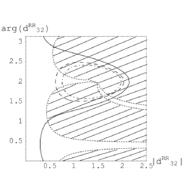
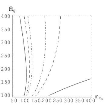
Figure 4: For large $\tilde{d}_{R}\tilde{s}_{R}$ mixing, the (dash-dot, dash, solid) curves are (0.9, 1.0, 1.25) contours of $|(C_{1}+\tilde{C}_{1})/C_{1}^{SM}|$, showing the NMFV contributions to $B_{d}\bar{B}_{d}$ mixing relative to the SM. $d_{32}^{RR}$ is defined in Eq. (7). The hatched region is excluded by $a_{\psi K_{s}}$. Parameters not shown on a plot’s axes are fixed as shown in Table 1.

However, if $\tilde{d}_{R}\tilde{s}_{R}$ mixing is small, the constraint on $\delta_{32}^{RR}$ from $B_{d}\bar{B}_{d}$ mixing is weak.

IV.3 $B_{s}\bar{B}_{s}$ mixing

$B_{s}\bar{B}_{s}$ mixing has not yet been observed and the current experimental limit is $\Delta m_{B_{s}}>14.4~{}ps^{-1}$ @ 95% C.L. Eidelman:2004wy . The SM prediction is: $14~{}{\rm ps^{-1}}<\Delta m_{B_{s}}<20~{}{\rm ps^{-1}}$ Anikeev:2001rk . The SM prediction for the dilepton asymmetry $A_{ll}^{B_{s}}$ is small, around $10^{-4}$, cf. references in Ref. Randall:1998te .

$B_{s}\bar{B}_{s}$ mixing depends quite sensitively on $\delta_{32}^{RR}$, and for the region in Fig. 4 allowed by $B_{d}\bar{B}_{d}$ mixing, we find $\Delta m_{B_{s}}\approx 22~{}{\rm ps^{-1}}$ and $A_{ll}^{B_{s}}\approx 5\times 10^{-4}$. This $\Delta m_{B_{s}}$ is a little higher than the SM prediction, although may be within the SM allowed range, given uncertainties.

As we pointed out in the previous subsection, if $\tilde{d}_{R}\tilde{s}_{R}$ mixing is small, then the $B_{d}\bar{B}_{d}$ mixing constraints on $\delta_{32}^{RR}$ becomes weak. If such is the case, there are essentially no constraints from $B_{d}\bar{B}_{d}$ mixing, and we show contours of $\Delta m_{B_{s}}$ and $A_{ll}^{B_{s}}$ in Fig. 5. We show only the range $(0<\arg{(\delta_{32}^{RR})}<\pi)$, since the $(\pi,~{}2\pi)$ range is identical to this. It can be seen that $\Delta m_{B_{s}}$ can increase significantly above the SM prediction.

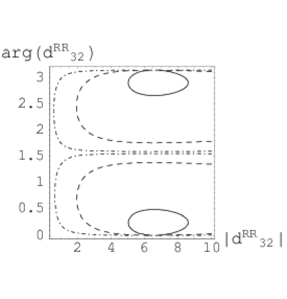
Figure 5: For small $\tilde{d}_{R}\tilde{s}_{R}$ mixing, the (dash-dot, dash, solid) curves are (15, 25, 40 ${\rm ps^{-1}}$) contours of $\Delta m_{B_{s}}$ (left), and ($10^{-4}$, $10^{-3}$ and $10^{-2}$) contours of $|A_{ll}^{B_{s}}|$ (right). $d_{32}^{RR}$ is defined in Eq. (7). Parameters not shown on a plot’s axes are fixed as shown in Table 1.

The projected Run II sensitivity for $\Delta m_{B_{s}}$ at the Tevatron with $2~{}{\rm fb^{-1}}$ is around $40~{}{\rm ps^{-1}}$ Anikeev:2001rk , and can probe a significant region of U(2) parameter space. If a higher value of $\Delta m_{B_{s}}$ is measured than what the SM predicts, it would indicate the presence of new physics. Measuring $A_{ll}^{B_{s}}$ can also significantly constrain $\delta_{32}^{RR}$ as can be seen from Fig. 5 (right).

V $\Delta B=1$ FCNC processes

V.1 Effective Hamiltonian

The $\Delta B=1$ effective Hamiltonian at a scale $\mu$ in the operator produce expansion (OPE) is Buchalla:1995vs ; Buras:1998ra ; Buras:1994dj

$${\cal H}^{eff}_{\Delta B=1}=-\frac{G_{F}}{\sqrt{2}}V_{ts}V_{tb}^{*}\left(\sum_{i=1...6,9,10}\!\!\!\!\!C_{i}(\mu)O_{i}(\mu)+C_{7\gamma}(\mu)O_{7\gamma}(\mu)+C_{8g}(\mu)O_{8g}(\mu)\right)\ ,$$ (33)

with

$$O_{1} = (\bar{s}_{\alpha}c_{\beta})_{V-A}(\bar{c}_{\beta}b_{\alpha})_{V-A},$$

$$O_{2} = (\bar{s}c)_{V-A}(\bar{c}b)_{V-A},$$

$$O_{3} = (\bar{s}b)_{V-A}\sum_{q}(\bar{q}q)_{V-A},$$

$$O_{4} = (\bar{s}_{\alpha}b_{\beta})_{V-A}\sum_{q}(\bar{q}_{\beta}q_{\alpha})_{V-A},$$

$$O_{5} = (\bar{s}b)_{V-A}\sum_{q}(\bar{q}q)_{V+A},$$

$$O_{6} = (\bar{s}_{\alpha}b_{\beta})_{V-A}\sum_{q}(\bar{q}_{\beta}q_{\alpha})_{V+A},$$

$$O_{7\gamma} = \frac{e}{8\pi^{2}}m_{b}\bar{s}_{\alpha}\sigma^{\mu\nu}(1+\gamma_{5})b_{\alpha}F_{\mu\nu},$$

$$O_{8g} = \frac{g_{s}}{8\pi^{2}}m_{b}\bar{s}_{\alpha}\sigma^{\mu\nu}(1+\gamma_{5})T^{a}_{\alpha\beta}b_{\beta}G^{a}_{\mu\nu},$$

$$O_{9} = (\bar{s}b)_{V-A}(\bar{e}e)_{V},$$

$$O_{10} = (\bar{s}b)_{V-A}(\bar{e}e)_{A},$$ (34)

where, the subscript $(V\pm A)$ means $\gamma_{\mu}(1\pm\gamma_{5})$, and $F^{\mu\nu}$, $G^{\mu\nu}$ are the electromagnetic and color field strengths, respectively.

The Wilson coefficients can be computed at the scale $M_{W}$ (the $W$ boson mass), and then run down to the scale $m_{b}$ (the $b$ quark mass). Below, when no scale is specified for the coefficients, it is understood to be at $m_{b}$, i.e., $C_{i}\equiv C_{i}(m_{b})$. The coefficients when run down from $M_{W}$ to $m_{b}$ mix under renormalization, so that Buras:xp  

$$C_{j} = \sum_{i=1}^{8}k_{ji}\eta^{a_{i}},\ \ \ \ (j=1,...,6),$$

$$C_{7\gamma} = \eta^{\frac{16}{23}}C_{7\gamma}(M_{W})+\frac{8}{3}\left(\eta^{\frac{14}{23}}-\eta^{\frac{16}{23}}\right)C_{8g}(M_{W})+\sum_{i=1}^{8}h_{i}\eta^{a_{i}}C_{2}(M_{W}),$$

$$C_{8g} = \eta^{\frac{14}{23}}C_{8g}(M_{W})+\sum_{i=1}^{8}\bar{h}_{i}\eta^{a_{i}}C_{2}(M_{W}),$$ (35)

where $\eta\equiv\frac{\alpha_{s}(M_{W})}{\alpha_{s}(m_{b})}\approx 0.56$ and $h_{i}$, $\bar{h}_{i}$, $a_{i}$ and $k_{ji}$ are given in Ref. Buchalla:1995vs . In addition, the evolution equation for $C_{9}$ is given in Ref. Buras:1994dj , and $C_{10}$ is not renormalized.

Separating out the new physics contribution to the renormalization group evolution, i.e., Eq. (35), we get

$$C_{2} = C_{2}^{SM},$$

$$C_{7\gamma} = C_{7\gamma}^{SM}+0.67C_{7\gamma}^{new}(M_{W})+0.09C_{8g}^{new}(M_{W}),$$

$$C_{8g} = C_{8g}^{SM}+0.70C_{8g}^{new}(M_{W}),$$ (36)

in which the superscript “SM” indicates the contribution from the SM, and “new” from new physics.

SM contribution: The SM $W^{\pm}$ contribution to $C_{7\gamma}(M_{W})$ and $C_{8g}(M_{W})$ are given by Grinstein:vj ; Demir:2001yz

$$C_{2}^{SM}(M_{W}) = 1,$$ (37)

$$C_{7\gamma,8g}^{SM}(M_{W}) = \frac{3}{2}F^{LL}_{7,8}\left(\frac{m_{t}^{2}}{M_{W}^{2}}\right),$$

where $F^{LL}_{7,8}(x)$ are given in Appendix B. Using Eq. (35) we can compute $C_{2}^{SM}$, $C_{7\gamma}^{SM}$ and $C_{8g}^{SM}$.

In the following, we will discuss, in order, the new physics contribution arising from the charged-Higgs boson ($H^{\pm}$), charginos ($\tilde{\chi}^{\pm}$) and gluinos ($\tilde{g}$).
Charged Higgs ($H^{\pm}$) contribution: The charged-Higgs contribution to $B_{d}\rightarrow X_{s}\gamma$ is given by Bertolini:1990if ; Demir:2001yz ; Barbieri:1993av

$$C_{7\gamma,8g}^{H}(M_{W}) = \frac{1}{2}\cot^{2}\beta F^{LL}_{7,8}\left(\frac{m_{t}^{2}}{M_{H}^{2}}\right)+\tilde{F}^{LL}_{7,8}\left(\frac{m_{t}^{2}}{M_{H}^{2}}\right),$$ (39)

where $F^{LL}_{7,8}(x)$ and $\tilde{F}^{LL}_{7,8}(x)$ are given in Appendix B.
Chargino ($\tilde{\chi}^{\pm}$) contribution: The chargino-stop contribution can be comparable to the SM contribution for a light stop and chargino. In the scenario that we are considering, the stop mixing angle is negligibly small and $m_{\tilde{t}_{L}}\approx m_{\tilde{t}_{1}}\sim\tilde{m}_{0}$ and $m_{\tilde{t}_{R}}\approx m_{\tilde{t}_{2}}\sim M_{W}$. We therefore run the $\tilde{t}_{1}$ contribution from $\tilde{m}_{0}$ down to $M_{W}$ and evaluate the $\tilde{t}_{2}$ contribution at $M_{W}$. The chargino-stop contribution is Bertolini:1990if ; Demir:2001yz ; Barbieri:1993av

$$C_{7\gamma,8g}^{\tilde{\chi}\tilde{t}_{1}}(\tilde{m}_{0})=-\sum_{j=1}^{2}\left[|\Gamma_{L}^{1j}|^{2}\frac{M_{W}^{2}}{m_{\tilde{t}_{1}}^{2}}F_{7,8}^{LL}\left(\frac{m_{\tilde{t}_{1}}^{2}}{M_{\tilde{\chi}_{j}}^{2}}\right)+\gamma_{RL}^{1j}\frac{M_{W}}{M_{\tilde{\chi}_{j}}}F_{7,8}^{RL}\left(\frac{m_{\tilde{t}_{1}}^{2}}{M_{\tilde{\chi}_{j}}^{2}}\right)\right],$$

$$C_{7\gamma,8g}^{\tilde{\chi}\tilde{t}_{2}}(M_{W})=-\sum_{j=1}^{2}\left[|\Gamma_{L}^{2j}|^{2}\frac{M_{W}^{2}}{m_{\tilde{t}_{2}}^{2}}F_{7,8}^{LL}\left(\frac{m_{\tilde{t}_{2}}^{2}}{M_{\tilde{\chi}_{j}}^{2}}\right)+\gamma_{RL}^{2j}\frac{M_{W}}{M_{\tilde{\chi}_{j}}}F_{7,8}^{RL}\left(\frac{m_{\tilde{t}_{2}}^{2}}{M_{\tilde{\chi}_{j}}^{2}}\right)\right],$$ (40)

where the loop functions $F_{7,8}^{RL}$ are given in Appendix B, and $\Gamma_{L}^{ij}$ and $\gamma_{RL}^{ij}$ contain the stop and chargino mixing matrices. Explicit expressions for $\Gamma_{L}^{ij}$, $\gamma_{RL}^{ij}$ and the renormalization group equations to evolve $C_{7\gamma,8g}^{\tilde{\chi}\tilde{t}_{1}}(\tilde{m}_{0})$ down to $M_{W}$ are given in Ref. Demir:2001yz .
Gluino ($\tilde{g}$) contribution: In our NMFV scenario, the gluino contributions can be sizable since they couple with strong interaction strength. Furthermore, because the sbottom mixing angle is negligibly small, $m_{\tilde{b}_{L}}\approx m_{\tilde{b}_{1}}\sim\tilde{m}_{0}$ and $m_{\tilde{b}_{R}}\approx m_{\tilde{b}_{2}}\sim M_{W}$. Keeping only the $\frac{M_{\tilde{g}}}{m_{b}}$ enhanced piece, the gluino contribution is Bertolini:1990if

$$C_{7\gamma}^{\tilde{g}}(M_{W})=-\frac{4\pi\alpha_{s}\sqrt{2}}{G_{F}V_{ts}^{*}V_{tb}}\frac{M_{\tilde{g}}}{m_{b}}\cos{\theta^{RL}_{32}}\sin{\theta^{RL}_{32}}e^{-i\gamma^{RL}_{32}}\frac{1}{9}\left[\frac{1}{m_{\tilde{b}_{2}}^{2}}F_{4}\left(\frac{M_{\tilde{g}}^{2}}{m_{\tilde{b}_{2}}^{2}}\right)-\frac{1}{m_{\tilde{b}_{1}}^{2}}F_{4}\left(\frac{M_{\tilde{g}}^{2}}{m_{\tilde{b}_{1}}^{2}}\right)\right],$$

$$C_{8g}^{\tilde{g}}(M_{W})=\frac{4\pi\alpha_{s}\sqrt{2}}{G_{F}V_{ts}^{*}V_{tb}}\frac{M_{\tilde{g}}}{m_{b}}\cos{\theta^{RL}_{32}}\sin{\theta^{RL}_{32}}e^{-i\gamma^{RL}_{32}}\frac{1}{8}\left[\frac{1}{m_{\tilde{b}_{2}}^{2}}F_{\tilde{g}}\left(\frac{M_{\tilde{g}}^{2}}{m_{\tilde{b}_{2}}^{2}}\right)-\frac{1}{m_{\tilde{b}_{1}}^{2}}F_{\tilde{g}}\left(\frac{M_{\tilde{g}}^{2}}{m_{\tilde{b}_{1}}^{2}}\right)\right],\$$ (41)

where the mixing angle $\theta^{RL}_{32}$ and phase $\gamma^{RL}_{32}$ are defined in Appendix A, and $F_{4}$ and $F_{\tilde{g}}$ are defined in Appendix B. In the above equation, we have neglected the effect of running the $\tilde{b}_{1}$ contribution from $\tilde{m}_{0}$ to $M_{W}$ as the $\tilde{b}_{2}$ contribution is dominant.

The dominant new physics contribution is given by adding Eqs. (39), (40) and (41), which yields

$$C_{7\gamma,8g}^{new}(M_{W})=C_{7\gamma,8g}^{H}(M_{W})+C_{7\gamma,8g}^{\tilde{\chi}}(M_{W})+C_{7\gamma,8g}^{\tilde{g}}(M_{W}).$$ (42)

In what follows we will discuss in detail the new physics contribution predicted by the U(2) model to the rare decay processes $B_{d}\rightarrow X_{s}\gamma$, $B_{d}\rightarrow X_{s}\,g$, $B_{d}\rightarrow X_{s}\ell^{+}\ell^{-}$ and $B_{d}\rightarrow\phi K_{s}$.

V.2 $B_{d}\rightarrow X_{s}\gamma$, $B_{d}\rightarrow X_{s}\,g$

The dominant operators contributing to $B_{d}\rightarrow X_{s}\gamma$ and $B_{d}\rightarrow X_{s}\,g$ are $O_{2}$, $O_{7\gamma}$ and $O_{8g}$. The decay branching ratio B.R.($B_{d}\rightarrow X_{s}\gamma$), at leading order, normalized to the semi-leptonic $B.R.(B_{d}\rightarrow X_{c}e\bar{\nu})\approx 10.5\%$, is given by Buras:xp ; mybsgwk ; Kagan:1998bh

$$\frac{\Gamma(B_{d}\rightarrow X_{s}\gamma)}{\Gamma(B_{d}\rightarrow X_{c}e\bar{\nu})}\Biggr{|}_{(E_{\gamma}>(1-\delta)E_{\gamma}^{max})}=\frac{6\alpha}{\pi}\frac{1}{g(\frac{m_{c}}{m_{b}})}\left|\frac{V^{*}_{ts}V_{tb}}{V_{cb}}\right|^{2}|C_{7\gamma}|^{2},$$ (43)

where $g(z)\equiv 1-8z^{2}+8z^{6}-z^{8}-24z^{4}\ln(z)$ is a phase space function, and $\delta$ is the fractional energy cut, i.e., only photon energy ${E_{\gamma}>(1-\delta)E_{\gamma}^{max}}$ is accepted.

The CP asymmetry in $B_{d}\rightarrow X_{s}\gamma$ is given by Kagan:1998bh

$$A_{CP}^{B_{d}\rightarrow X_{s}\gamma}(\delta) = \frac{\Gamma(\bar{B}_{d}\rightarrow X_{s}\gamma)-\Gamma(B_{d}\rightarrow X_{\bar{s}}\gamma)}{\Gamma(\bar{B}_{d}\rightarrow X_{s}\gamma)+\Gamma(B_{d}\rightarrow X_{\bar{s}}\gamma)}\Biggr{|}_{E_{\gamma}>(1-\delta)E_{\gamma}^{max}}\ ,$$ (44)

$$= \frac{1}{|C_{7\gamma}|^{2}}\{{a_{27}(\delta){\rm Im}[C_{2}C_{7\gamma}^{*}]+a_{87}(\delta){\rm Im}[C_{8g}C_{7\gamma}^{*}]+a_{28}(\delta){\rm Im}[C_{2}C_{8g}^{*}]}\}.$$

For $\delta=0.15$, which is a typical experimental cut, we use $a_{27}=0.0124$, $a_{87}=-0.0952$ and $a_{28}=0.0004$ Kagan:1998bh .

The experimentally measured HFAG branching ratio is $B.R.(B_{d}\rightarrow X_{s}\gamma)=(3.52^{+0.3}_{-0.28})\times 10^{-4}$. In the SM, we have $C_{2}^{SM}\approx 1.11$, $C_{7\gamma}^{SM}\approx-0.31$ and $C_{8g}^{SM}\approx-0.15$. The SM prediction for B.R.($B_{d}\rightarrow X_{s}\gamma$), which depends on $|C_{7\gamma}|$, cf. Eq. (43), is largely consistent with experiment, and new physics contributions to $|C_{7\gamma}|$ is constrained by this branching ratio. In the context of SUSY this has been analyzed, for example, in Refs. Bertolini:1990if ; Buras:xp ; mybsgwkbr .

The SM CP asymmetry in $B_{d}\rightarrow X_{s}\gamma$ is of the order of 1%, so that a larger CP asymmetry measured would imply new physics Kagan:1998bh . The present limit at 95 % C.L. is HFAG ; Nishida:2003yw ; Aubert:2004hq $-0.07<A_{CP}^{B_{d}\rightarrow X_{s}\gamma}<0.07$.

The B.R.($B_{d}\rightarrow X_{s}\,g$) is obtained simply from Eq. (43)

$$\frac{\Gamma(B_{d}\rightarrow X_{s}\,g)}{\Gamma(B_{d}\rightarrow X_{c}e\bar{\nu})}=C(R)\frac{6\alpha_{s}}{\pi}\frac{1}{g(\frac{m_{c}}{m_{b}})}\left|\frac{V^{*}_{ts}V_{tb}}{V_{cb}}\right|^{2}|C_{8g}|^{2},$$ (45)

where the SU(3) quadratic Casimir $C(R)=4/3$. The B.R.($B_{d}\rightarrow X_{s}\,g$) has large experimental and theoretical uncertainties and Ref. Kagan:1997qn suggests that the data might prefer a B.R. value of around $10\%$.

Figs. 6 and 7 show the interplay between the $W^{\pm}$, $H^{\pm}$, $\tilde{\chi}^{\pm}$ and $\tilde{g}$ contributions to $B_{d}\rightarrow X_{s}\gamma$, where the sum of these contributions to the magnitude of $C_{7\gamma}$ is constrained by B.R.($B_{d}\rightarrow X_{s}\gamma$). The experimental data on B.R.($B_{d}\rightarrow X_{s}\gamma$) allows (at $2\,\sigma$) the region bounded by the contours shown in the figures. In the plots, the parameters are as given in Table 1, and some relevant ones are varied as shown in the figures.

To illustrate the dependence on the MFV parameters, we consider for example, in Fig. 6, the dependence of $A_{CP}^{B_{d}\rightarrow X_{s}\gamma}$ and B.R.($B_{d}\rightarrow X_{s}\gamma$) as a function of $m_{H}$ and $M_{2}$ (left) and as a function of $\tan\beta$ and $\arg{(\mu)}$ (right), for the choice of parameters shown in Table 1. The experimental $2\,\sigma$ allowed contours of B.R.($B_{d}\rightarrow X_{s}\gamma$) are also shown.

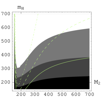
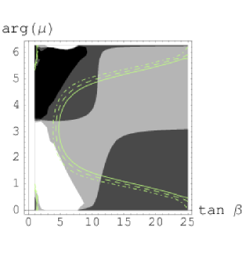
Figure 6: The boundaries between the shaded regions show (2.5,3,3.5)% (darkest to lightest) contours of $A_{CP}^{B_{d}\rightarrow X_{s}\gamma}$ as a function of $m_{H}$ and $M_{2}$ (left), and, (-3.5,0,3.5)% (darkest to lightest) contours of $A_{CP}^{B_{d}\rightarrow X_{s}\gamma}$ as a function of $\tan\beta$ and $\arg{(\mu)}$ (right). Superimposed is the experimental $2\,\sigma$ allowed contours of B.R.($B_{d}\rightarrow X_{s}\gamma$). Parameters not shown on a plot’s axes are fixed as shown in Table 1.

In Fig. 7 (left), the shaded regions show $A_{CP}^{B_{d}\rightarrow X_{s}\gamma}$ as a function of the magnitude and argument of $d_{32}^{RL}$, the dimensionless $\mathcal{O}(1)$ coefficient defined in Eq (8). In Fig. 7 (right), we show contours of B.R.($B_{d}\rightarrow X_{s}\,g$), and a B.R. of up to about 15% can be accommodated in this model.

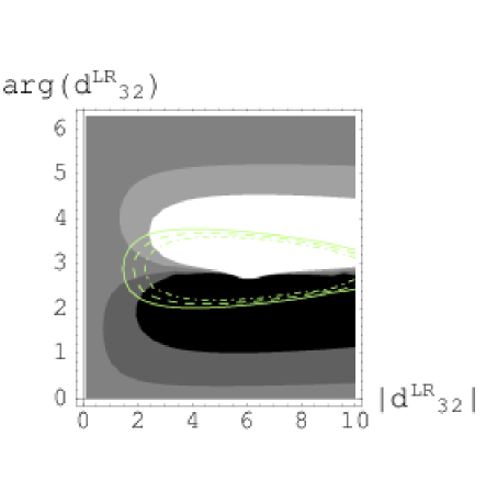
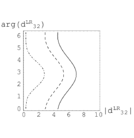
Figure 7: The boundaries between the shaded regions show (-7,-3,3,7)% (darkest to lightest) contours of $A_{CP}^{B_{d}\rightarrow X_{s}\gamma}$ (left) with experimentally allowed $2\,\sigma$ contours of B.R.($B_{d}\rightarrow X_{s}\gamma$) superimposed, and, 1 %, 7.5 % and 15 % contours of predicted B.R.($B_{d}\rightarrow X_{s}\,g$) (right). Parameters not shown on a plot’s axes are fixed as shown in Table 1.

V.3 $B_{d}\rightarrow X_{s}\ell^{+}\ell^{-}$

The dominant operators contributing to $B_{d}\rightarrow X_{s}\ell^{+}\ell^{-}$ ($\ell=e,\mu$) are $O_{7\gamma}$, $O_{9}$ and $O_{10}$. It is usual to define

$$C_{9}(\mu) \equiv \frac{\alpha}{2\pi}\tilde{C}_{9}(\mu),$$

$$C_{10} \equiv \frac{\alpha}{2\pi}\tilde{C}_{10},$$

and

$$\hat{s}\equiv\frac{(p_{\ell^{+}}+p_{\ell^{-}})^{2}}{m_{b}^{2}}.$$ (46)

The (differential) partial width $\frac{d}{d\hat{s}}\Gamma(B_{d}\rightarrow X_{s}\ell^{+}\ell^{-})$, normalized to $\Gamma(B_{d}\rightarrow X_{c}e\bar{\nu})$, is given by Buras:1994dj :

$$R(\hat{s})\equiv\frac{\frac{d}{d\hat{s}}\Gamma(B_{d}\rightarrow X_{s}\ell^{+}\ell^{-})}{\Gamma(B_{d}\rightarrow X_{c}e\bar{\nu})}=\frac{\alpha^{2}}{4\pi^{2}}\left|\frac{V_{ts}^{*}V_{tb}}{V_{cb}}\right|^{2}\frac{(1-\hat{s})^{2}}{f(\frac{m_{c}}{m_{b}})\kappa(\frac{m_{c}}{m_{b}})}\left[(1+2\hat{s})\left(|\tilde{C}_{9}^{eff}|^{2}+|\tilde{C}_{10}|^{2}\right)+\right.$$

$$\left.4\left(1+\frac{2}{\hat{s}}\right)|C_{7\gamma}|^{2}+12~{}{\rm Re}(C_{7\gamma}\tilde{C}_{9}^{eff})\right],$$ (47)

where $f$ and $\kappa$ are phase space functions and $\tilde{C}_{9}^{eff}$ is the QCD corrected $\tilde{C}_{9}$, given in terms of $\tilde{C}_{9}$ and $C_{i}$ ($i$=1…6) Buras:1994dj . Integrating this we get the prediction for the decay branching ratios and we show this in Table 2 for the SM along with the experimental result HFAG . We choose the lower limit on the integration to correspond to a typical experimental choice, $(p_{\ell^{+}}+p_{\ell^{-}})^{2}>(0.2~{}{\rm GeV})^{2}$. Since the rate of $B_{d}\rightarrow X_{s}\ell^{+}\ell^{-}$ is down by the square of the electromagnetic coupling constant compared to $B_{d}\rightarrow X_{s}\gamma$, the experimental errors are comparatively larger.

	ExperimentHFAG	SM prediction
$B.R.(B_{d}\rightarrow X_{s}\ell^{+}\ell^{-})$	$4.46^{+0.98}_{-0.96}\times 10^{-6}$	$5.3\times 10^{-6}$

Table 2: The current data for $B_{d}\rightarrow X_{s}\ell^{+}\ell^{-}$.

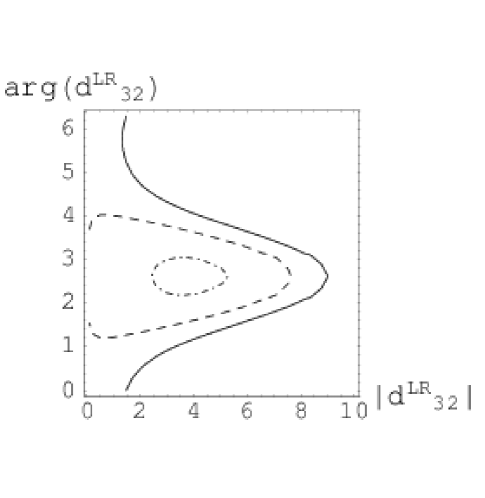
Figure 8: The (dash-dot, dash, solid) curves are $(5.25,~{}6.25,~{}7.25)\times 10^{-6}$ contours of $B_{d}\rightarrow X_{s}\ell^{+}\ell^{-}$. Parameters not shown on the plot’s axes are fixed as shown in Table 1.

Fig. 8 shows the contours of B.R.($B_{d}\rightarrow X_{s}\ell^{+}\ell^{-}$) as a function of $d_{32}^{RL}$. Compared to B.R.($B_{d}\rightarrow X_{s}\gamma$), cf. Fig. 7 (left), the $B_{d}\rightarrow X_{s}\ell^{+}\ell^{-}$ constraint is not very stringent right now, and improved statistics at the B-factories could place tighter constraints on the parameter space.

V.4 $B_{d}\rightarrow\phi K_{s}$

The decay $B_{d}\rightarrow\phi K_{s}$ ($b\rightarrow ss\bar{s}$ at the quark level) can be a sensitive probe of new physics since the leading order SM contribution is one-loop suppressed, and loop processes involving heavy SUSY particles can contribute significantly. However, the computation of B.R.($B_{d}\rightarrow\phi K_{s}$) suffers from significant theoretical uncertainties in calculating the hadronic matrix elements. We follow the factorization approach, details of which are presented in Ref. Beneke:2001ev . The theoretical uncertainties largely cancel in the CP asymmetry, and is therefore a good probe of new physics.

The CP asymmetry in $B_{d}\rightarrow\phi K_{s}$ is defined by

$$A_{CP}^{B_{d}\rightarrow\phi K_{s}} \equiv \frac{\Gamma\left(\bar{B}_{d}(t)\rightarrow\phi K_{s}\right)-\Gamma\left(B_{d}(t)\rightarrow\phi K_{s}\right)}{\Gamma\left(\bar{B}_{d}(t)\rightarrow\phi K_{s}\right)+\Gamma\left(B_{d}(t)\rightarrow\phi K_{s}\right)}$$ (48)

$$= -C_{\phi K}\cos{\left(\Delta m_{B_{d}}\,t\right)}+S_{\phi K}\sin{\left(\Delta m_{B_{d}}\,t\right)}\ ,$$ (49)

where

$$C_{\phi K} \equiv \frac{1-|\lambda_{\phi K}|^{2}}{1+|\lambda_{\phi K}|^{2}}\ ,$$

$$S_{\phi K} \equiv \frac{2\,{\rm Im}{\left(\lambda_{\phi K}\right)}}{1+|\lambda_{\phi K}|^{2}}\ ,$$

$$\lambda_{\phi K} \equiv -e^{-2i(\beta+\theta_{d})}\frac{\bar{A}(B_{d}\rightarrow\phi K_{s})}{A(\bar{B_{d}}\rightarrow\phi K_{s})}\ ,$$

where $B_{d}(t)$ represents the state that is a $B_{d}$ at time $t=0$, $\Delta m_{B_{d}}$ is the $B_{d}\bar{B}_{d}$ mass difference, $\beta$ is the usual angle in the SM CKM unitarity triangle fits to the CP asymmetry in $B_{d}\rightarrow J/\psi~{}K_{s}$, and $\theta_{d}$ is any new physics contributions to $B_{d}\bar{B}_{d}$ mixing ($\theta_{d}$ is discussed in Section IV.2). The SM predicts that the CP asymmetry in $B_{d}\rightarrow\phi K_{s}$ and $B_{d}\rightarrow J/\psi~{}K_{s}$ should be the same, i.e., $S_{\phi K}=\sin{2\beta}$.

The $\bar{B_{d}}\rightarrow\phi K_{s}$ amplitude and partial decay width are given by Kane:2002sp ; Beneke:2001ev :

$$A(\bar{B_{d}}\rightarrow\phi K_{s}) = \sum_{p=u,c}\lambda_{p}\left[(a_{3}+a_{4}^{p}+a_{5})-\frac{1}{2}(a_{7}+a_{9}+a_{10}^{p})\right]$$ (50)

$$\Gamma(\bar{B_{d}}\rightarrow\phi K_{s}) = \frac{G_{F}^{2}f_{\phi}^{2}m_{B}^{3}}{32\pi}(F_{1}^{B\rightarrow K})^{2}|A(\bar{B_{d}}\rightarrow\phi K_{s})|^{2}\left[\lambda(1,\frac{m_{\phi}^{2}}{m_{B}^{2}},\frac{m_{K}^{2}}{m_{B}^{2}})\right]^{\frac{3}{2}}$$ (51)

where the phase space function $\lambda(x,y,z)\equiv x^{2}+y^{2}+z^{2}-2xy-2yz-2zx$, the $\phi$ decay constant $f_{\phi}=237$ MeV, the form factor $F_{1}^{B\rightarrow K}=0.38$ and $\lambda_{p}\equiv V_{pb}V_{ps}^{*}$. The SM $a_{i}$’s, in terms of the $C_{i}$’s, are given in Ref. Beneke:2001ev to which we add the new physics contribution given in Eq. (42). We do not include the power-suppressed weak annihilation operators and we refer the reader to Refs. Beneke:2001ev  and Beneke:2003zv for a more complete discussion. As explained in Section. II.2, we are only including the $\delta_{32}^{RL}$ SUSY contribution, as this is the dominant one. The amplitude for the CP conjugate process $B_{d}\rightarrow\phi K_{s}$ is obtained by taking $\lambda_{p}\rightarrow\lambda_{p}^{*}$.

The current $B_{d}\rightarrow\phi K_{s}$ experimental average HFAG is summarized in Table. 3. The SM requires $S_{\phi K}=S_{J/\psi K}\equiv\sin{2\beta}$, but the experimental data has about a $2\,\sigma$ discrepancy between $S_{\phi K}$ and $S_{J/\psi K}$. Though not convincing yet, this could be an indication of new physics and we ask if this can be naturally explained in the theory we are considering.

	Experiment HFAG	SM prediction
$B.R.(B_{d}\rightarrow\phi K_{s})$	$8.3^{+1.2}_{-1.0}\times 10^{-6}$	$\sim 5\times 10^{-6}$
$S_{\phi K}$	$0.34\pm 0.2$	$0.725\pm 0.037$
$C_{\phi K}$	$-0.04\pm 0.17$	$0$

Table 3: The current data for $B_{d}\rightarrow\phi K_{s}$.

We showed in Section IV.2, that if $\tilde{d}_{R}\tilde{s}_{R}$ mixing is small, there is no significant new phase in $M_{12}(B_{d})$ (i.e., $\theta_{d}\approx 0$). For this case, we scan the parameter space $\arg(\mu)$, $|\delta_{32}^{RL}|$, $\arg(\delta_{32}^{RL})$, and in Fig. 9 show a scatter-plot of the points that satisfy all experimental constraints including B.R.($B_{d}\rightarrow X_{s}\gamma$) and B.R.($B_{d}\rightarrow\phi K_{s}$).

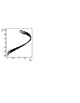
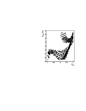
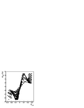
Figure 9: $A_{CP}^{B_{d}\rightarrow X_{s}\gamma}$, $S_{\phi K}$ and $C_{\phi K}$ for points that satisfy all experimental constraints (within $2\,\sigma$), resulting from a scan over $d_{32}^{LR}$ and ${\rm arg}(\mu)$, for small $\tilde{d}_{R}\tilde{s}_{R}$ mixing (negligible $\theta_{d}$). All other parameters are fixed as shown in Table 1.

We find that it is possible to satisfy all experimental constraints including the recent $B_{d}\rightarrow\phi K_{s}$ data shown in Table 3 in the framework we are considering. Furthermore, there are strong correlations between $A_{CP}^{B_{d}\rightarrow X_{s}\gamma}$, $S_{\phi K}$ and $C_{\phi K}$. As the accuracy of the experimental data improve, we can use these correlations to (in)validate the choices that we make in our model.

Large $\tilde{d}_{R}\tilde{s}_{R}$ mixing can lead to a nonzero $\theta_{d}$ which depends on $|\delta_{32}^{RR}|$ as explained in Section IV.2. We therefore include this new phase and perform a scan over $|\delta_{32}^{RR}|$, $\arg(\delta_{32}^{RR})$, $\arg(\mu)$, $|\delta_{32}^{RL}|$ and $\arg(\delta_{32}^{RL})$. We show the points that satisfy all experimental constraints and the resulting $A_{CP}^{B_{d}\rightarrow X_{s}\gamma}$, $S_{\phi K}$ and $C_{\phi K}$ in Fig. 10.

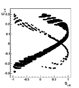
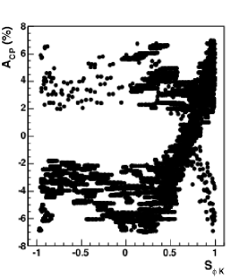
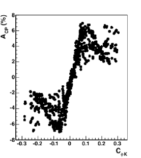
Figure 10: $A_{CP}^{B_{d}\rightarrow X_{s}\gamma}$, $S_{\phi K}$ and $C_{\phi K}$ for points that satisfy all experimental constraints (within $2\,\sigma$), resulting from a scan over $d_{32}^{LR,RR}$ and ${\rm arg}(\mu)$, for large $\tilde{d}_{R}\tilde{s}_{R}$ mixing (nonzero $\theta_{d}$). All other parameters are fixed as shown in Table 1.

We again see from Fig. 10 that $A_{CP}^{B_{d}\rightarrow X_{s}\gamma}$, $S_{\phi K}$ and $C_{\phi K}$ are strongly correlated, although the effect of the new phase in $B_{d}\bar{B}_{d}$ mixing allows new regions of parameter space compared to the small mixing case shown in Fig. 9. Even in the case of large mixing we find that it is possible to satisfy all experimental data including the $S_{\phi K}$ and $C_{\phi K}$. One feature that we find in either large or small mixing case is that sign $(C_{\phi K})$ is positively correlated with sign $(A_{CP}^{B_{d}\rightarrow X_{s}\gamma})$. Thus, further data could shed light on the validity of the choices that we make in our model.

VI Conclusions

A supersymmetric U(2) theory has the potential to explain the gauge hierarchy and flavor problems in the SM. We assumed an effective SUSY mass spectrum just above the weak scale, the only relatively light scalars being the right handed stop and sbottom (weak scale masses). We analyzed what such a hypothesis would imply for $K$ and $B$ meson observables by including all the dominant contributions that can interfere in a certain observable. Although for definiteness we considered a U(2) framework, our conclusions hold for any theory with a similar SUSY mass spectrum and structure of the squark mass matrix.

The CP violation parameter in Kaon mixing, $\epsilon_{K}$, can impose constraints on the MFV parameter space of our model, as we showed in Fig. 2, while the gluino contribution to $\epsilon_{K}$ is negligible. There is sufficient room to accommodate the MFV contributions to $\epsilon_{K}$, given the present uncertainty in the lattice computation of the Bag parameter $B_{K}$.

We find that $B_{d}\bar{B}_{d}$ mixing and $a_{\psi K_{s}}$ ($\sin{2\beta}$) can impose constraints on the supersymmetric U(2) theory. In addition to the MFV contribution, if $\tilde{d}_{R}\tilde{s}_{R}$ mixing is large, the gluino contributions to $B_{d}\bar{B}_{d}$ mixing can be significant leading to a strong constraint on the 32 entry of the RR squark mass matrix, $\delta_{32}^{RR}$, as shown in Fig. 4. Furthermore, in this case, there is a new phase in the $B_{d}\bar{B}_{d}$ mixing amplitude coming from the SUSY sector. However, if $\tilde{d}_{R}\tilde{s}_{R}$ mixing is small, the constraint on $\delta_{32}^{RR}$ from $B_{d}\bar{B}_{d}$ mixing is weak.

$B_{s}\bar{B}_{s}$ mixing most sensitively depends on $\delta_{32}^{RR}$ in the SUSY U(2) theory. If $\delta_{32}^{RR}$ is unconstrained by $B_{d}\bar{B}_{d}$ mixing (small $\tilde{d}_{R}\tilde{s}_{R}$ mixing), we showed that $\Delta m_{B_{s}}$ can be increased to quite large values (up to about $40~{}{\rm ps^{-1}}$), cf. Fig. 5 . The current and upcoming experiments can reach sensitivities required to see the SM prediction for $\Delta m_{B_{s}}$. Seeing a higher value, or not seeing a signal at all, might hint at some new physics of the type we are considering. We also presented expectations for the $B_{s}$ dilepton asymmetry, $A_{ll}^{B_{s}}$, which can constrain $\delta_{32}^{RR}$.

The experimental data on B.R.($B_{d}\rightarrow X_{s}\gamma$) imposes a constraint on the SUSY theory. While satisfying this constraint, we showed that an enhancement in CP Violation in $B_{d}\rightarrow X_{s}\gamma$ is possible. Since in the SM, $A_{CP}^{B_{d}\rightarrow X_{s}\gamma}$ is predicted to be less than $1\%$, if a much larger value is measured, it would clearly point to new physics. In Fig. 7 we presented the expectations for $A_{CP}^{B_{d}\rightarrow X_{s}\gamma}$ and B.R.($B_{d}\rightarrow X_{s}\,g$) while varying the magnitude and phase of $\delta_{32}^{RL}$. We also presented expectations for B.R.($B_{d}\rightarrow X_{s}\ell^{+}\ell^{-}$) in Fig. 8.

The present experimental data on the CP violation in $B_{d}\rightarrow\phi K_{s}$ has about a $2\,\sigma$ deviation from the SM prediction, and it will be very interesting to see if this would persist with more data. We showed that such a deviation can be accommodated in the framework we are considering, both for large or small $\tilde{d}_{R}\tilde{s}_{R}$ mixing. We showed, in Fig. 10, that $A_{CP}^{B_{d}\rightarrow X_{s}\gamma}$ can be enhanced significantly while satisfying all other experimental bounds including the present data on $S_{\phi K}$ and $C_{\phi K}$. In Figs. 9 and 10, for small and large $\tilde{d}_{R}\tilde{s}_{R}$ mixing respectively, we see strong correlations between $A_{CP}^{B_{d}\rightarrow X_{s}\gamma}$, $S_{\phi K}$ and $C_{\phi K}$. Comparing these with upcoming data with improved precision could shed light on the validity of the choices that we make in our model.

We conclude by remarking that the prospects are exciting for discovering SUSY in B-meson processes at current and upcoming colliders. Here, we showed this for a SUSY U(2) model. To unambiguously establish that it is a SUSY U(2) theory, and to determine the various SUSY breaking parameters, will require looking at a broad range of observables.

Appendix A Mixing Angles

The charged SU(2) Majorana gauginos $\tilde{W}_{1}$, $\tilde{W}_{2}$ can be combined to form the Dirac spinor

$$\tilde{W}^{+}=\frac{1}{\sqrt{2}}\pmatrix{{\tilde{W}^{+}}_{\alpha}\cr{\tilde{W}^{-\,\dot{\alpha}}}}\ ,$$ (52)

where $\tilde{W}^{\pm}_{\alpha}=\tilde{W}_{1\alpha}\pm i\tilde{W}_{2\alpha}$. The up and down type Higgsinos can be combined to form the Dirac spinor

$$\tilde{H}^{+}=\pmatrix{\tilde{H}_{u\,\alpha}\cr\tilde{H}_{d}^{\dot{\alpha}}}\ .$$ (53)

The chargino mass terms can then be written as

$${\cal L}\supset-\pmatrix{\overline{\tilde{W}^{+}}&\overline{\tilde{H}^{+}}}\left({\cal M}_{\chi}~{}P_{L}+{\cal M}_{\chi}^{\dagger}~{}P_{R}\right)\pmatrix{\tilde{W}^{+}\cr\tilde{H}^{+}}\ ,$$ (54)

where

$${\cal M}_{\chi}=\pmatrix{M_{2}&\sqrt{2}\sin{\beta}~{}m_{W}\cr\sqrt{2}\cos{\beta}~{}m_{W}&\mu}\ .$$ (55)

We can go to the chargino mass eigen basis $(\chi_{1}\ \chi_{2})$ by making the rotations

$$P_{L,R}\pmatrix{\tilde{W}^{+}\cr\tilde{H}^{+}}=\left({\cal C}_{L,R}\right)~{}P_{L,R}\pmatrix{\tilde{\chi}_{1}^{+}\cr\tilde{\chi}_{2}^{+}}\ ,$$ (56)

with the rotation matrices ${\cal C}_{L,R}$ given as

$${\cal C}_{\alpha}=\pmatrix{\cos\theta_{\alpha}&-\sin\theta_{\alpha}~{}e^{-i\gamma_{\alpha}}\cr\sin\theta_{\alpha}~{}e^{i\gamma_{\alpha}}&\cos\theta_{\alpha}}\pmatrix{e^{i\eta_{\alpha}}&0\cr 0&e^{i\rho_{\alpha}}}\ ,$$ (57)

where the mixing angles and phases are Demir:2001yz

$$\gamma_{L} = -\arg{\left(M_{2}+\mu\cot\beta\right)}$$ (58)

$$\tan{2\theta_{L}} = \frac{\sqrt{8}\,m_{W}\sin\beta|M_{2}+\mu\cot\beta|}{M_{2}^{2}+|\mu|^{2}+2\,m_{W}^{2}\cos{2\beta}}$$

$$\gamma_{R} = -\arg{\left(M_{2}+\mu^{*}\tan\beta\right)}$$

$$\tan{2\theta_{R}} = \frac{\sqrt{8}\,m_{W}\cos\beta|M_{2}+\mu^{*}\tan\beta|}{M_{2}^{2}-|\mu|^{2}-2\,m_{W}^{2}\cos{2\beta}}$$

$$\eta_{R} = \arg\left(c_{R}(M_{2}c_{L}+\sqrt{2}m_{W}\sin\beta s_{L}e^{i\gamma_{L}})+s_{R}e^{-i\gamma_{R}}(\sqrt{2}m_{W}\cos\beta c_{L}+\mu s_{L}e^{i\gamma_{L}})\right)$$

$$\rho_{R} = \arg\left(c_{R}(-\sqrt{2}m_{W}\cos\beta s_{L}e^{-i\gamma_{L}}-\mu c_{L})+s_{R}e^{i\gamma_{R}}(-M_{2}s_{L}e^{-i\gamma_{L}}+\sqrt{2}m_{W}\sin\beta c_{L})\right)$$

with $0\leq\theta_{\alpha}\leq\pi/2$ so that $M_{\alpha_{1}}^{2}>M_{\alpha_{2}}^{2}$, and, $s_{L,R}\equiv\sin\theta_{L,R}$ and $c_{L,R}\equiv\cos\theta_{L,R}$.

The sbottom mass terms are given as, cf. Eq. (5)

$${\cal L}\supset-\pmatrix{\tilde{b}_{L}^{*}&\tilde{b}_{R}^{*}}\pmatrix{m_{3LL}^{2}+m_{b}^{2}+\Delta_{L}^{d}&(v_{d}A_{b}-\mu^{*}\tan{\beta}~{}m_{b})^{*}\cr v_{d}A_{b}-\mu^{*}\tan{\beta}~{}m_{b}&m_{\tilde{b}_{R}}^{2}+m_{b}^{2}+\Delta_{R}^{d}}\pmatrix{\tilde{b}_{L}\cr\tilde{b}_{R}}\ ,$$ (59)

where the $\Delta_{L,R}$ are the D-term contributions given as

$$\Delta^{d}=\left(T_{3}-Q_{EM}\sin^{2}\theta_{W}\right)\cos{2\beta}m_{Z}^{2}\ .$$ (60)

This is diagonalized by the rotation

$$\pmatrix{\tilde{b}_{L}\cr\tilde{b}_{R}} = \pmatrix{\cos{\theta_{\tilde{b}}}&-\sin{\theta_{\tilde{b}}}e^{-i\gamma_{\tilde{b}}}\cr\sin{\theta_{\tilde{b}}}e^{i\gamma_{\tilde{b}}}&\cos{\theta_{\tilde{b}}}}\pmatrix{\tilde{b}_{1}\cr\tilde{b}_{2}}$$ (61)

$$\equiv \left({\cal C}_{\tilde{b}}\right)\pmatrix{\tilde{b}_{1}\cr\tilde{b}_{2}}\ ,$$

where the mixing angle and phase are given by

$$\tan{2\theta_{\tilde{b}}} = \frac{2|v_{d}A_{b}-\mu^{*}\tan{\beta}~{}m_{b}|}{(m_{3LL}^{2}+\Delta_{L}^{d})-(m_{\tilde{b}_{R}}^{2}+\Delta_{R}^{d})}\ ,$$

$$\gamma_{\tilde{b}} = \arg{(v_{d}A_{b}-\mu^{*}\tan{\beta}~{}m_{b})}\ .$$ (62)

We have similar equations for stop mixing with obvious changes, in addition to the off diagonal term now being given as: ($v_{u}A_{t}-\mu^{*}\cot{\beta}~{}m_{t}$), and the stop mixing matrix denoted as ${\cal C}_{\tilde{t}}$. In our framework, owing to the smallness of the off diagonal RL mixing term compared to $m_{3LL}^{2}\sim m_{0}^{2}$, we have small stop and sbottom mixing. Furthermore, the sbottom mixing angle is negligibly small and we neglect its mixing effects. We thus have $\tilde{b}_{1}\approx\tilde{b}_{L}$ and $\tilde{b}_{2}\approx\tilde{b}_{R}$. The stop mixing angle, however, is not as small and so we include its effects.

To compute the interaction vertices in the SuperKM basis, one could diagonalize the $6\times 6$ squark mass matrix. Since the off-diagonal entries in our case are small, we perform an approximate leading order diagonalization of the mass matrices shown in Eq. (5).

Focusing first on the $\tilde{b}_{R}\tilde{s}_{L}$ mixing,

$${\cal L}\supset-\pmatrix{\tilde{s}_{L}^{*}&\tilde{b}_{R}^{*}}\pmatrix{m_{1LL}^{2}+\epsilon^{2}m_{2LL}^{2}+m_{s}^{2}+\Delta_{L}^{d}&(v_{d}A_{4}^{\prime}\epsilon)^{*}\cr v_{d}A_{4}^{\prime}\epsilon&m_{\tilde{b}_{R}}^{2}+m_{b}^{2}+\Delta_{R}^{d}}\pmatrix{\tilde{s}_{L}\cr\tilde{b}_{R}}\ .$$ (63)

This is diagonalized by the rotation

$$\pmatrix{\tilde{s}_{L}\cr\tilde{b}_{R}} = \pmatrix{\cos{\theta_{32}^{RL}}&-\sin{\theta_{32}^{RL}}e^{-i\gamma_{32}^{RL}}\cr\sin{\theta_{32}^{RL}}e^{i\gamma_{32}^{RL}}&\cos{\theta_{32}^{RL}}}\pmatrix{\tilde{q}_{2}\cr\tilde{q}_{3}}$$ (64)

$$\equiv \left({\cal C}_{\tilde{b}_{R}\tilde{s}_{L}}\right)\pmatrix{\tilde{q}_{2}\cr\tilde{q}_{3}}\ .$$

The mixing angle and phase are given by

$$\tan{2\theta_{32}^{RL}} = \frac{2|v_{d}A\epsilon|}{(m_{1LL}^{2}+m_{s}^{2}+\Delta_{L}^{d})-(m_{\tilde{b}_{R}}^{2}+m_{b}^{2}+\Delta_{R}^{d})}\ ,$$

$$\gamma_{32}^{RL} = \arg{(v_{d}A\epsilon)}\ .$$ (65)

The $\tilde{b}_{R}\tilde{s}_{R}$ mixing is given similarly. We have the mass terms

$${\cal L}\supset-\pmatrix{\tilde{s}_{R}^{*}&\tilde{b}_{R}^{*}}\pmatrix{m_{1RR}^{2}+m_{s}^{2}+\Delta_{R}^{d}&(\epsilon m_{4}^{2})^{*}\cr\epsilon m_{4}^{2}&m_{\tilde{b}_{R}}^{2}+m_{b}^{2}+\Delta_{R}^{d}}\pmatrix{\tilde{s}_{R}\cr\tilde{b}_{R}}\ ,$$ (66)

which is diagonalized by the rotation

$$\pmatrix{\tilde{s}_{R}\cr\tilde{b}_{R}} = \pmatrix{\cos{\theta_{32}^{RR}}&-\sin{\theta_{32}^{RR}}e^{-i\gamma_{32}^{RR}}\cr\sin{\theta_{32}^{RR}}e^{i\gamma_{32}^{RR}}&\cos{\theta_{32}^{RR}}}\pmatrix{\tilde{q}_{2}\cr\tilde{q}_{3}}$$ (67)

$$\equiv \left({\cal C}_{\tilde{b}_{R}\tilde{s}_{R}}\right)\pmatrix{\tilde{q}_{2}\cr\tilde{q}_{3}}\ .$$

The mixing angle and phase are given by

$$\tan{2\theta_{32}^{RR}} = \frac{2|\epsilon m_{4}^{2}|}{(m_{1RR}^{2}+m_{s}^{2}+\Delta_{R}^{d})-(m_{\tilde{b}_{R}}^{2}+m_{b}^{2}+\Delta_{R}^{d})}\ ,$$

$$\gamma_{32}^{RR} = \arg{(\epsilon m_{4}^{2})}\ .$$ (68)

The $\tilde{d}_{L}\tilde{s}_{L}$ and $\tilde{d}_{R}\tilde{s}_{R}$ mixing terms are

$${\cal L}\supset-\pmatrix{\tilde{d}_{L,R}^{*}&\tilde{s}_{L,R}^{*}}\pmatrix{m_{1}^{2}+m_{d}^{2}+\Delta_{L,R}^{d}&i\epsilon^{\prime}m_{5}^{2}\cr-i\epsilon^{\prime}m_{5}^{2}&m_{1}^{2}+m_{s}^{2}+\epsilon^{2}m_{2}^{2}+\Delta_{L,R}^{d}}_{LL,RR}\pmatrix{\tilde{d}_{L,R}\cr\tilde{s}_{L,R}}\ .$$ (69)

The matrices that diagonalizes these, ${\mathcal{C}}_{\tilde{d}_{L}\tilde{s}_{L}}$ and ${\mathcal{C}}_{\tilde{d}_{R}\tilde{s}_{R}}$ are given analogous to Eq. (67), the angle and phase ($\theta_{12}^{LL}$, $\gamma_{12}^{LL}$) and ($\theta_{12}^{RR}$, $\gamma_{12}^{RR}$) given analogous to Eq. (68), and we will not write them down explicitly. The diagonal entries are split only by $\mathcal{O}(\epsilon^{2})$, and therefore this mixing is maximal in general. However, if $\epsilon^{\prime}m_{5}^{2}\ll\epsilon^{2}m_{2}^{2}$, this mixing can be small.

Appendix B Loop functions

The $B_{d}\rightarrow X_{s}\gamma$ loop functions are given by

$$F^{LL}_{7}(x) = \left(\frac{x(7-5x-8x^{2})}{36(x-1)^{3}}+\frac{x^{2}(3x-2)}{6(x-1)^{4}}\ln{x}\right)\ ,$$

$$F^{LL}_{8}(x) = \left(\frac{x(2+5x-x^{2})}{12(x-1)^{3}}-\frac{3x^{2}}{6(x-1)^{4}}\ln{x}\right)\ ,$$

$$F^{RL}_{7}(x) = \left(\frac{5-7x}{6(x-1)^{2}}+\frac{x(3x-2)}{3(x-1)^{3}}\ln{x}\right)\ ,$$

$$F^{RL}_{8}(x) = \left(\frac{1+x}{2(x-1)^{2}}-\frac{x}{(x-1)^{3}}\ln{x}\right)\ ,$$

$$\tilde{F}^{LL}_{7}(x) = \left(\frac{x(3-5x)}{12(x-1)^{2}}+\frac{x(3x-2)}{6(x-1)^{3}}\ln{x}\right)\ ,$$

$$\tilde{F}^{LL}_{8}(x) = \left(\frac{x(3-x)}{4(x-1)^{2}}-\frac{x}{2(x-1)^{3}}\ln{x}\right)\ .$$ (70)

$$F_{4}(x) = \frac{x^{2}-1-2x\ln{x}}{2(x-1)^{3}}$$

$$F_{\tilde{g}}(x) = -\frac{5x^{2}-18x+13+(9-x)\ln{x}}{3(x-1)^{3}}$$ (71)

The SM box functions are given by

$$S_{0}(x) = \frac{4x-11x^{2}+x^{3}}{4(1-x)^{2}}-\frac{3x^{3}\ln{x}}{2(1-x)^{3}}\ ,$$

$$S_{0}(x_{1},x_{2}) = \frac{x_{1}x_{2}}{4}\biggl{\{}\frac{x_{1}^{2}-8x_{1}+4}{(x_{1}-x_{2})(x_{1}-1)^{2}}\ln{x_{1}}+\frac{x_{2}^{2}-8x_{2}+4}{(x_{2}-x_{1})(x_{2}-1)^{2}}\ln{x_{2}}$$ (72)

$$~{}~{}~{}\biggl{.}-\frac{3}{(x_{1}-1)(x_{2}-1)}\biggl{\}}\ .$$

The charged-Higgs and chargino box functions are given by

$$Y_{1}(r_{\alpha},r_{\beta},s_{i},s_{j})=\frac{r_{\alpha}^{2}}{(r_{\beta}-r_{\alpha})(s_{i}-r_{\alpha})(s_{j}-r_{\alpha})}\ln{r_{\alpha}}+\frac{r_{\beta}^{2}}{(r_{\alpha}-r_{\beta})(s_{i}-r_{\beta})(s_{j}-r_{\beta})}\ln{r_{\beta}}$$

$$+\frac{s_{i}^{2}}{(r_{\alpha}-s_{i})(r_{\beta}-s_{i})(s_{j}-s_{i})}\ln{s_{i}}+\frac{s_{j}^{2}}{(r_{\alpha}-s_{j})(r_{\beta}-s_{j})(s_{i}-s_{j})}\ln{s_{j}}\ ,$$

$$Y_{2}(r_{\alpha},r_{\beta},s_{i},s_{j})=\sqrt{s_{i}s_{j}}\left[\frac{r_{\alpha}}{(r_{\beta}-r_{\alpha})(s_{i}-r_{\alpha})(s_{j}-r_{\alpha})}\ln{r_{\alpha}}+\frac{r_{\beta}}{(r_{\alpha}-r_{\beta})(s_{i}-r_{\beta})(s_{j}-r_{\beta})}\ln{r_{\beta}}\right.$$

$$\left.+\frac{s_{i}}{(r_{\alpha}-s_{i})(r_{\beta}-s_{i})(s_{j}-s_{i})}\ln{s_{i}}+\frac{s_{j}}{(r_{\alpha}-s_{j})(r_{\beta}-s_{j})(s_{i}-s_{j})}\ln{s_{j}}\right]\ .$$ (73)

from which various limiting cases can be obtained.

The gluino box integrals are given as

$$I_{4}\equiv I_{4}(M_{\tilde{g}}^{2},M_{\tilde{g}}^{2},m_{\tilde{b}_{R}}^{2},m_{\tilde{b}_{R}}^{2})=\int\!\frac{d^{4}p}{(2\pi)^{4}}~{}\frac{1}{(p^{2}-M_{\tilde{g}}^{2})(p^{2}-M_{\tilde{g}}^{2})(p^{2}-m_{\tilde{b}_{R}}^{2})(p^{2}-m_{\tilde{b}_{R}}^{2})}\ ,$$

$$\tilde{I}_{4}\equiv\tilde{I}_{4}(M_{\tilde{g}}^{2},M_{\tilde{g}}^{2},m_{\tilde{b}_{R}}^{2},m_{\tilde{b}_{R}}^{2})=\int\!\frac{d^{4}p}{(2\pi)^{4}}~{}\frac{p^{2}}{(p^{2}-M_{\tilde{g}}^{2})(p^{2}-M_{\tilde{g}}^{2})(p^{2}-m_{\tilde{b}_{R}}^{2})(p^{2}-m_{\tilde{b}_{R}}^{2})}\ ,$$ (74)

which we evaluate numerically using LoopTools Hahn:1998yk in Mathematica.

References

- (1) A. G. Cohen, D. B. Kaplan and A. E. Nelson, “The more minimal supersymmetric standard model,” Phys. Lett. B 388, 588 (1996) [hep-ph/9607394].
- (2) A. Pomarol and D. Tommasini, “Horizontal symmetries for the supersymmetric flavor problem,” Nucl. Phys. B 466, 3 (1996) [hep-ph/9507462].
- (3) R. Barbieri, G. R. Dvali and L. J. Hall, “Predictions From A U(2) Flavour Symmetry In Supersymmetric Theories,” Phys. Lett. B 377, 76 (1996) [hep-ph/9512388]; R. Barbieri, L. J. Hall and A. Romanino, “Consequences of a U(2) flavour symmetry,” Phys. Lett. B 401, 47 (1997) [hep-ph/9702315].
- (4) G. Degrassi, P. Gambino and G. F. Giudice, “B X/s gamma in supersymmetry: Large contributions beyond the leading order,” JHEP 0012, 009 (2000) [hep-ph/0009337]; M. Carena, D. Garcia, U. Nierste and C. E. Wagner, “b s gamma and supersymmetry with large tan(beta),” Phys. Lett. B 499, 141 (2001) [hep-ph/0010003].
- (5) S. Bertolini, F. Borzumati, A. Masiero and G. Ridolfi, “Effects Of Supergravity Induced Electroweak Breaking On Rare B Decays And Mixings,” Nucl. Phys. B 353, 591 (1991).
- (6) J. S. Hagelin, S. Kelley and T. Tanaka, “Supersymmetric flavor changing neutral currents: Exact amplitudes and phenomenological analysis,” Nucl. Phys. B 415, 293 (1994).
- (7) L. J. Hall, V. A. Kostelecky and S. Raby, “New Flavor Violations In Supergravity Models,” Nucl. Phys. B 267, 415 (1986); F. Gabbiani and A. Masiero, “FCNC In Generalized Supersymmetric Theories,” Nucl. Phys. B 322, 235 (1989); F. Gabbiani, E. Gabrielli, A. Masiero and L. Silvestrini, “A complete analysis of FCNC and CP constraints in general SUSY extensions of the standard model,” Nucl. Phys. B 477, 321 (1996) [hep-ph/9604387]; M. Misiak, S. Pokorski and J. Rosiek, “Supersymmetry and FCNC effects,” Adv. Ser. Direct. High Energy Phys. 15, 795 (1998) [hep-ph/9703442].
- (8) G. L. Kane, P. Ko, H. b. Wang, C. Kolda, J. h. Park and L. T. Wang, “B/d Phi K(S) and supersymmetry,” Phys. Rev. D 70, 035015 (2004) [hep-ph/0212092]; K. Agashe and C. D. Carone, “Supersymmetric flavor models and the B Phi K(S) anomaly,” Phys. Rev. D 68, 035017 (2003) [hep-ph/0304229].
- (9) T. Affolder et al. [CDF Collaboration], “Search for scalar top and scalar bottom quarks in p anti-p collisions at Phys. Rev. Lett. 84, 5704 (2000) [hep-ex/9910049]; C. Rott, “Searches for the Supersymmetric Partner of the Bottom Quark,” hep-ex/0410007.
- (10) S. Eidelman et al. [Particle Data Group Collaboration], “Review of particle physics,” Phys. Lett. B 592, 1 (2004).
- (11) G. Buchalla, A. J. Buras and M. E. Lautenbacher, “Weak Decays Beyond Leading Logarithms,” Rev. Mod. Phys. 68, 1125 (1996) [hep-ph/9512380].
- (12) G. C. Branco, G. C. Cho, Y. Kizukuri and N. Oshimo, “Supersymmetric contributions to B0 - anti-B0 and K0 - anti-K0 mixings,” Phys. Lett. B 337, 316 (1994) [hep-ph/9408229]; “Searching for signatures of supersymmetry at B factories,” Nucl. Phys. B 449, 483 (1995).
- (13) D. Becirevic et al., “B/d anti-B/d mixing and the B/d J/psi K(S) asymmetry in general SUSY models,” Nucl. Phys. B 634, 105 (2002) [hep-ph/0112303].
- (14) A. J. Buras and R. Fleischer, “Quark mixing, CP violation and rare decays after the top quark discovery,” Adv. Ser. Direct. High Energy Phys. 15, 65 (1998) [hep-ph/9704376].
- (15) P. Ko, J. h. Park and G. Kramer, “B0 - anti-B0 mixing, B J/psi K(S) and B X/d gamma in general MSSM,” Eur. Phys. J. C 25, 615 (2002) [hep-ph/0206297].
- (16) L. Randall and S. f. Su, “CP violating lepton asymmetries from B decays and their implication for supersymmetric flavor models,” Nucl. Phys. B 540, 37 (1999) [hep-ph/9807377].
- (17) We use the (ICHEP 2004) average from CLEO, BaBar and Belle compiled by the Heavy Flavor Averaging group. http://www.slac.stanford.edu/xorg/hfag/
- (18) Y. Grossman, Y. Nir and M. P. Worah, “A model independent construction of the unitarity triangle,” Phys. Lett. B 407, 307 (1997) [hep-ph/9704287].
- (19) G. C. Branco, L. Lavoura and J. P. Silva, “CP Violation,” Clarendon Press, Oxford (1999).
- (20) K. Anikeev et al., “B physics at the Tevatron: Run II and beyond,” [hep-ph/0201071].
- (21) A. J. Buras, “Weak Hamiltonian, CP violation and rare decays,” [hep-ph/9806471].
- (22) A. J. Buras and M. Munz, “Effective Hamiltonian for B X(s) e+ e- beyond leading logarithms in the NDR and HV schemes,” Phys. Rev. D 52, 186 (1995) [hep-ph/9501281].
- (23) A. J. Buras, M. Misiak, M. Munz and S. Pokorski, “Theoretical Uncertainties And Phenomenological Aspects Of B X(S) Gamma Decay,” Nucl. Phys. B 424, 374 (1994) [hep-ph/9311345].
- (24) K. G. Chetyrkin, M. Misiak and M. Munz, “Weak radiative B-meson decay beyond leading logarithms,” Phys. Lett. B 400, 206 (1997) [Erratum-ibid. B 425, 414 (1998)] [hep-ph/9612313].
- (25) B. Grinstein, R. P. Springer and M. B. Wise, “Effective Hamiltonian For Weak Radiative B Meson Decay,” Phys. Lett. B 202, 138 (1988).
- (26) D. A. Demir and K. A. Olive, “B X/s gamma in supersymmetry with explicit CP violation,” Phys. Rev. D 65, 034007 (2002) [hep-ph/0107329].
- (27) R. Barbieri and G. F. Giudice, “b s gamma decay and supersymmetry,” Phys. Lett. B 309, 86 (1993) [hep-ph/9303270].
- (28) A. Ali, H. Asatrian and C. Greub, “Inclusive decay rate for B X/d + gamma in next-to-leading logarithmic order and CP asymmetry in the standard model,” Phys. Lett. B 429, 87 (1998) [hep-ph/9803314]; A. L. Kagan and M. Neubert, “QCD anatomy of B X/s gamma decays,” Eur. Phys. J. C 7, 5 (1999) [hep-ph/9805303].
- (29) A. L. Kagan and M. Neubert, “Direct CP violation in B X/s gamma decays as a signature of new physics,” Phys. Rev. D 58, 094012 (1998) [hep-ph/9803368].
- (30) S. Bertolini, F. Borzumati and A. Masiero, “Supersymmetric Enhancement Of Noncharmed B Decays,” Nucl. Phys. B 294, 321 (1987); R. Barbieri and G. F. Giudice, “b s gamma decay and supersymmetry,” Phys. Lett. B 309, 86 (1993) [hep-ph/9303270]; P. L. Cho, M. Misiak and D. Wyler, “ and Decay in the MSSM,” Phys. Rev. D 54, 3329 (1996) [hep-ph/9601360]. J. L. Hewett and J. D. Wells, “Searching for supersymmetry in rare B decays,” Phys. Rev. D 55, 5549 (1997) [hep-ph/9610323].
- (31) S. Nishida et al. [BELLE Collaboration], “Measurement of the CP asymmetry in B X/s gamma,” Phys. Rev. Lett. 93, 031803 (2004) [hep-ex/0308038].
- (32) B. Aubert et al. [BABAR Collaboration], “Measurement of the direct CP asymmetry in b s gamma decays,” Phys. Rev. Lett. 93, 021804 (2004) [hep-ex/0403035].
- (33) A. L. Kagan and J. Rathsman, “Hints for enhanced b s g from charm and kaon counting,” [hep-ph/9701300].
- (34) J. Kaneko et al. [Belle Collaboration], “Measurement of the electroweak penguin process B X/s l+ l-,” Phys. Rev. Lett. 90, 021801 (2003) [hep-ex/0208029].
- (35) M. Beneke, G. Buchalla, M. Neubert and C. T. Sachrajda, “QCD factorization in B pi K, pi pi decays and extraction of Wolfenstein parameters,” Nucl. Phys. B 606, 245 (2001) [hep-ph/0104110].
- (36) M. Beneke and M. Neubert, “QCD factorization for B P P and B P V decays,” Nucl. Phys. B 675, 333 (2003) [hep-ph/0308039].
- (37) B. Aubert et al. [BABAR Collaboration], “Measurement of sin(2beta) in B0 Phi K0(S). ((B)),” hep-ex/0207070.
- (38) K. Abe et al. [Belle Collaboration], “An improved measurement of mixing-induced CP violation in the neutral B meson system,” hep-ex/0207098.
- (39) T. Hahn and M. Perez-Victoria, “Automatized one-loop calculations in four and D dimensions,” Comput. Phys. Commun. 118, 153 (1999) [hep-ph/9807565].