A New SUSY mass reconstruction method at the CERN LHC

Abstract

We propose a new mass reconstruction technique for SUSY processes at the LHC. The idea is to completely solve the kinematics of the SUSY cascade decay by using the assumption that the selected events satisfy the same mass shell conditions of the sparticles involved in the cascade decay. Using this technique, we study the measurement of the mass of the bottom squarks in the cascade decay of the gluino. Based on the final state including two high $p_{T}$ leptons and two $b$-jets, we investigate different possible approaches to the mass reconstruction of the gluino and the two bottom squarks. In particular we evaluate the performance of different algorithms in discriminating two bottom squark states with a mass difference as low as 5%.

I INTRODUCTION

Supersymmetry is one of the most attractive models beyond the Standard Model (SM) of elementary particle physics. The superpartners of SM particles (sparticles) might have masses of the order of the TeV, and experiments at the Large Hadron Collider (LHC) should be able to detect such particles up to masses of 2-3 TeV atltdr ; Abdullin:1998pm .

The pattern of the sparticle mass spectrum depends on the SUSY-breaking mechanism, which might depend on gravity, space-time structure, or unknown interactions. The unraveling of such mechanism through the determination of the sparticles’ masses is therefore one of the most important physics targets of future collider experiments.

The potential of the LHC for SUSY mass determination has been studied in detail in the past decade. The most promising method involves the study of the endpoints in the distributions of invariant masses among the visible sparticle decay products. Information on the masses involved in the cascade decay can be extracted from the endpoint values if the decay distributions are dominated by a single cascade decay chain. Studies based on the endpoints are documented in atltdr ; Hinchliffe:1997iu ; Hinchliffe:1999zc ; Bachacou:1999zb ; Allanach:2000kt ; Abdullin:1998pm ; gjelsten .

In this paper we explore a new method for reconstructing SUSY events. This method does not rely only on events near the endpoint. Instead, one kinematically solves the neutralino momenta and masses of heavier sparticles using measured jet and lepton momenta and optionally a few mass inputs.

We concentrate in this paper on the measurement of the mass of the bottom squarks (sbottoms) through the cascade decay:

$$\tilde{g}\rightarrow\tilde{b}b_{2}\rightarrow\tilde{\chi}^{0}_{2}b_{1}b_{2}\rightarrow\tilde{\ell}b_{1}b_{2}\ell_{2}\rightarrow\tilde{\chi}^{0}_{1}b_{1}b_{2}\ell_{1}\ell_{2}.$$ (1)

We address this decay, rather than the equivalent cascade involving a generic $\tilde{q}_{L}$ for various orders of reasons. First of all, the physics of the third generation squarks and leptons is particularly important in disentangling the pattern of SUSY breaking. In the MSUGRA model, $\tilde{b}_{L}$ is lighter than $\tilde{b}_{R}$ due to the RGE running by top Yukawa coupling. The mass of the lighter sbottom state $\tilde{b}_{1}$ is further reduced by the mixing of the left and right $\tilde{b}$ states. The sbottom sector is thus sensitive to fundamental parameters of the theory such as the trilinear couplings and $\tan\beta$ otherwise of difficult access at the LHC. The third generation sparticle masses are also important parameters for $B$ and Higgs physics. Second, the chain in Eq. (1) involves two $b$ quarks, which can be tagged in the detector. The problem of correctly identifying the jets contributing to the interesting decay is thus made much simpler. Finally, as we will discuss in detail below, both sbottom states $\tilde{b}_{1}$ and $\tilde{b}_{2}$ yield the decay chain of Eq. (1). The performance and the robustness of the reconstruction algorithms can be benchmarked against the ability in disentangling the two states.

Five sparticles are involved in the cascade decay Eq. (1), therefore one can write five mass shell conditions among the leptons and quarks in the final decay products.

$$m^{2}_{\tilde{\chi}^{0}_{1}} = p^{2}_{\tilde{\chi}^{0}_{1}},$$ (2)

$$m^{2}_{\tilde{\ell}} = (p_{\tilde{\chi}^{0}_{1}}+p_{\ell_{1}})^{2},$$ (3)

$$m^{2}_{\tilde{\chi}^{0}_{2}} = (p_{\tilde{\chi}^{0}_{1}}+p_{\ell_{1}}+p_{\ell_{2}})^{2},$$ (4)

$$m^{2}_{\tilde{b}} = (p_{\tilde{\chi}^{0}_{1}}+p_{\ell_{1}}+p_{\ell_{2}}+p_{b_{1}})^{2},$$ (5)

$$m^{2}_{\tilde{g}} = (p_{\tilde{\chi}^{0}_{1}}+p_{\ell_{1}}+p_{\ell_{2}}+p_{b_{1}}+p_{b_{2}})^{2}.$$ (6)

For a $bb\ell\ell$ event, the equations contain the 4 unknown degrees of freedom of the $\tilde{\chi}^{0}_{1}$ momentum. Each event therefore describes a 4-dimensional hyper-surface in a 5-dimensional mass parameter space, and the hyper-surface differs event by event. From the purely mathematical point of view 5 events would be enough to determine a discrete set of solutions for the masses of the involved sparticles, and the probabilistic discussion of the following could be easily developed in a 5-dimensional space. In order to illustrate the method in a more transparent way, we will develop the argument by assuming that the masses of $\tilde{\chi}^{0}_{2}$, $\tilde{\ell}$, and $\tilde{\chi}^{0}_{1}$ are known. This is a reasonable assumption at the LHC, where it has been shown that a detailed study of the lepton-lepton system from the $\tilde{\chi}^{0}_{2}$ decay can be used to precisely constrain these masses Nojiri:2000wq . In this case, each event corresponds to a different line in the $(m_{\tilde{g}},m_{\tilde{b}})$ plane, therefore two events are enough to solve the gluino and sbottom masses altogether.

We call this technique the “mass relation method”, because here one uses the fact that sparticle masses are common for all events which go though the same cascade decay chain. Note that the events need not to be close to the endpoint of the decay distribution, but they are still relevant to the mass determination. This means that one can use the mass relation method even if the number of signal events is small.

The purpose of this paper is to explore in detail the implications of the mass relation method which is only sketched for signal events in Nojiri:2003tu . In that report a measurement of the gluino and sbottom masses was obtained from the peak of the distribution of the solutions for all possible event pairs, assuming that the $\tilde{\chi}^{0}_{2}$, $\tilde{\ell}$ and $\tilde{\chi}^{0}_{1}$ masses are known. In this paper we extend the previous analysis to take SUSY backgrounds into account in the distributions.

We note that $\tilde{b}$ in Eq. (1) could be either $\tilde{b}_{1}$ or $\tilde{b}_{2}$. The decay was studied in gjelsten by using the endpoint method, where the possibility of distinguishing the two sbottom states $\tilde{b}_{1}$ and $\tilde{b}_{2}$ was studied for a case where the mass difference was approximately 5% of the sbottom mass. The conclusion showed that even with very large integrated luminosity the result is at best marginal, and crucially depends on the ability of the experimenters to model to a very high level of detail the response function of the detector to $b$-jets. This is probably an inescapable conclusion, given that the resolution in calorimetric measurement is comparable to the mass splitting one wants to measure. It is however worth studying alternative reconstruction methods which make a better use of all the information available for the selected events.

In a subsequent paper Lester , a similar process is analyzed by constructing an approximate event-likelihood function for signal events, based on a Bayesian statistical approach. In this paper we construct a different approximation for the likelihood function. We apply this function to the analysis of a simulated data set, and we study how well $\tilde{b}_{1}$ and $\tilde{b}_{2}$ can be reconstructed for a sample model point and its variants.

This paper is organized as follows. In section II, we introduce the detailed SUSY models addressed in our study, and briefly present the simulation procedure. We then solve in section III analytically the kinematics for the process Eq. (1), arriving to a compact expression for the masses of $\tilde{g}$ and $\tilde{b}$ as the function of $b$ and $\ell$ momentum and discuss the typical solutions. In section V, we discuss the event pair analysis on our sample SUSY model, where $m_{\tilde{g}}$ and $m_{\tilde{b}}$ are computed from all event pairings in the selected samples. Gluino and sbottom masses consistent with the input values are reconstructed, but we are also forced to artificially select one of the multiple solutions obtained from solving for the masses the coupled quadratic equations for each event pair. In section VI, we therefore define an approximate likelihood function built using all the events in the sample, and we describe an analysis based on this function. The masses reconstructed from the likelihood analysis are in agreement with the input values and the method automatically takes care of the issue of multiple solutions without artificial selection. We also study the possibility to reconstruct the $\tilde{b}_{2}$ in our sample model. Section VII is devoted to discussions and comments. We especially discuss the theoretical relevance of being able to perform detailed measurements in the third generation squark sector.

II Model points and simulations

We choose for this study the model point SPS1a as defined in Ref. Allanach:2002nj and its variants. SPS1a has a significant production cross-section for the chain of Eq. (1), and has already been the subject of detailed LHC studies gjelsten . The model is defined in the mSUGRA scenario by the parameters $\tan\beta=10$, $m=100$ GeV, $M=250$ GeV, $A_{0}=-100$ GeV, and $\mu>0$. In order to evaluate the performance of the analysis for different values of the splitting of the two sbottom states, we also study the points where $\tan\beta=15$ and $20$, keeping other GUT scale parameters same as those for SPS1a. For the additional points, the ${\tilde{g}}$, $\tilde{\chi}^{0}_{2}$, $\tilde{\chi}^{0}_{1}$ and $\tilde{\ell}$ masses are almost the same as for SPS1a, while $m_{\tilde{b}_{1}}$ is reduced because the left right mixing of $\tilde{b}$ increases proportional to $\mu\tan\beta$.

The masses and decay branching ratios are calculated with the ISASUSY code ISASUSY . The $m_{\tilde{b}_{1}}$ changes by 3% from $\tan\beta=10$ to $\tan\beta=20$. We will see later that such a difference in the $\tilde{b}_{1}$ masses should be measurable at the LHC if systematic effects are kept under control.

Another drastic effect in Table 2 is the decrease of $Br(\tilde{\chi}^{0}_{2}\rightarrow\tilde{\ell}\ell)$ ($\ell=e,\mu$). This is because the decay width for $\tilde{\chi}^{0}_{2}\rightarrow\tilde{\tau}\tau$ increases as the $\tilde{\tau}$ mixing angle increases. For $\tan\beta=20$, the branching ratio into $bb\ell\ell$ mode is reduced by a factor of 5 yielding a rather small number of accepted events.

We also list in Table 2 the decay branching ratios relevant to the decay chain of our interest. The ratio of the decay branching ratios $R_{\tilde{b}}=Br(\tilde{g}\rightarrow\tilde{b}_{2}\rightarrow\tilde{\chi}^{0}_{2})/$$Br(\tilde{g}\rightarrow\tilde{b}_{1}\rightarrow\tilde{\chi}^{0}_{2})$ varies from 0.26 to 0.14 when $\tan\beta$ changes from 10 to 20. This $\tan\beta$ dependence comes from the reduction of $\tilde{b}_{1}$ mass and the increase of the left-right mixing of $\tilde{b}$, $\theta$, defined as $\tilde{b}_{1}\equiv\cos\theta\tilde{b}_{L}+\sin\theta\tilde{b}_{R}$, from $\theta=0.49$ ($\tan\beta=10$) to 0.61 ($\tan\beta=20$). Namely,

• $\Gamma(\tilde{g}\rightarrow\tilde{b}_{1})$ increases as $m_{\tilde{b}_{1}}$ is reduced.

• $\Gamma(\tilde{b}_{2}\rightarrow\tilde{\chi}^{0}_{2})$ increases as $\theta$ increases. However, $\Gamma(\tilde{b}_{2}\rightarrow\tilde{\chi}^{+}_{1})$ and $\Gamma(\tilde{b}_{2}\rightarrow\tilde{t}_{1})$ also increase, therefore $Br(\tilde{b}_{2}\rightarrow\tilde{\chi}^{0}_{2})$ stays more or less same.

• $m_{\tilde{b}_{1}}$ is reduced and $\Gamma(\tilde{b}_{1}\rightarrow\tilde{t}_{1}W)$ is kinematically suppressed as $\tan\beta$ increases.

The branching ratio is in principle important information to determine the mixing angle $\theta$ but one needs to know the relevant sparticle mass spectrum to utilize it.

Note that the ratio $R_{\tilde{b}}$ is small and the mass splitting between $\tilde{b}_{1}$ and $\tilde{b}_{2}$ is within 10% over the parameters we study. The $\tilde{b}_{1}$ is therefore significant background for the $\tilde{b}_{2}$ search at the LHC. Nevertheless, a hint for the decay of $\tilde{g}\rightarrow\tilde{b}_{2}$ might still be observable in the $bb\ell\ell$ distribution, given an excellent control of the detector response to $b$-jets, as we will see in section VI.

The SUSY events are generated using the HERWIG 6.4 Corcella:2000bw ; Moretti:2002eu event generator. The produced events are passed through the ATLFAST ATLFAST detector simulator, which parameterizes the response of the ATLAS detector. In particular, we use the parametrization for $b$-tagging efficiency corresponding to the expected high luminosity performance of the ATLAS detector. While the performance is a function of the $p_{T}$ of the jets, a typical performance figure is $\epsilon_{b}=0.5$ for the $b$ tagging efficiency for a rejection of 100 on light quark jets.

For each point we have generated $1.5\times 10^{7}$ events which approximately correspond to an integrated luminosity of 300 fb^-1.

The following cuts are applied in order to select signal events:

• $M_{\rm eff}>600$ GeV and $E_{T}^{\rm miss}>0.2M_{\rm eff}$, where $E_{T}^{\rm miss}$ is the missing transverse energy and $M_{\rm eff}$ is the scalar sum of the missing transverse energy and the transverse momenta of the four hardest jets,

• at least 3 jets with $p_{T1}>150$ GeV, $p_{T2}>100$ GeV and $p_{T3}>50$ GeV,

• exactly two $b$-tagged jets with $p_{T}>50$ GeV,

• exactly two opposite-sign isolated same-flavor (OSSF) leptons with $p_{T\ell_{1}}>20$ GeV, $p_{T\ell_{2}}>10$ GeV, with an invariant mass $40$ GeV$<m_{\ell\ell}<78$ GeV.

The isolation criterion consists in requiring a transverse energy deposition in the calorimeters smaller than $10$ GeV in a ($\eta,\phi$) cone of radius $0.2$ around the lepton direction, where $\eta$ is the pseudorapidity of the lepton and $\phi$ the angle in the plane transverse to the beam. A detailed discussion of the Standard Model backgrounds after these cuts is given in gjelsten . The authors show that the Standard Model background is negligible in comparison to the SUSY background, consisting of SUSY events not including the decay chain of Eq. (1).

In order to perform the reconstruction, we need to identify the position of each of the two $b$-jets and of each of the two leptons in the decay chain. In the following analysis, we assume that the $b$-jet with larger $p_{T}$ originates from the $\tilde{b}$ decay. The assignment is optimal for SPS1a, because $m_{\tilde{b}}-m_{\tilde{\chi}^{0}_{2}}\gg m_{\tilde{g}}-m_{\tilde{b}}$. At the same time one can fix the lepton assignment so that the higher (lower) $p_{T}$ lepton $\ell_{\rm high}$ ($\ell_{\rm low}$) comes from $\tilde{\ell}$ to increase the possibility to pick up the correct lepton assignment. If we roughly know the masses of $\tilde{\ell},\tilde{\chi}^{0}_{1}$ and $\tilde{\chi}^{0}_{2}$, it is easy to determine which assignment is optimal Nojiri:2000wq . For the likelihood analysis on SPS1a, we use $\ell_{\rm high}$ as $\ell_{1}$ in Eq. (1).

$\tan\beta$	$m_{\tilde{g}}$	$m_{\tilde{b}_{1(2)}}$	$m_{\tilde{\chi}^{0}_{2}}$	$m_{\tilde{\ell}_{R}}$	$m_{\tilde{\chi}^{0}_{1}}$
10	595.2	491.9 (524.6)	176.8	143.0	96.0
15	595.2	485.3 (526.9)	177.9	143.0	96.5
20	595.2	478.7 (531.2)	178.5	143.1	96.7

Table 1: Masses of the relevant sparticles for the three studied points, in GeV.

$\tan\beta$	$Br({\tilde{g}}\to\tilde{b}_{1(2)})$	$Br(\tilde{b}_{1(2)}\to\tilde{\chi}_{2}^{0})$	$Br(\tilde{\chi}_{2}^{0}\to\tilde{\ell})$
10	8.9 (4.9) $\times$2	35.8 (16.7)	3.16$\times$4
15	9.8 (4.6) $\times$2	37.8 (15.9)	1.26$\times$4
20	10.8 (4.1) $\times$2	38.9 (13.2)	0.61$\times$4

Table 2: Branching fractions for the decays used in the analysis, in percent.

III Solutions of the decay kinematics

III.1 Formula of the decay kinematics

It is straightforward to solve the decay process in Eq. (1). We first note that the $\tilde{b}$ cascade decay can be written as a function of momenta of $b_{1}$, $\ell_{1}$ and $\ell_{2}$ , because the four mass shell conditions can be used to eliminate the unknown $\tilde{\chi}^{0}_{1}$ four momentum.

To systematically solve the system, we expand the $\tilde{\chi}^{0}_{1}$ momentum with the observed momenta of $b_{1}$, $\ell_{1}$, and $\ell_{2}$:

$$\vec{\rm p}_{\tilde{\chi}^{0}_{1}}=a\vec{\rm p}_{\ell_{1}}+b\vec{\rm p}_{\ell_{2}}+c\vec{\rm p}_{b_{1}}.$$ (7)

The expansion is possible if $\vec{\rm p}_{\ell_{1}}$, $\vec{\rm p}_{\ell_{2}}$ and $\vec{\rm p}_{b_{1}}$ are independent from one another. The three on-shell conditions may be then rewritten as

$${\cal M}\left(\begin{array}[]{c}a\cr b\cr c\end{array}\right)=\left(\begin{array}[]{lll}-\frac{1}{2}(m_{\tilde{\ell}}^{2}-m_{\tilde{\chi}^{0}_{1}}^{2})&&+E_{\ell_{1}}E_{\tilde{\chi}^{0}_{1}}\cr-\frac{1}{2}(m_{\tilde{\chi}^{0}_{2}}^{2}-m_{\tilde{\ell}}^{2}-2p_{\ell_{1}}\cdot p_{\ell_{2}})&&+E_{\ell_{2}}E_{\tilde{\chi}^{0}_{1}}\cr\frac{1}{2}\left(m_{\tilde{\chi}^{0}_{2}}^{2}+m_{b}^{2}+2p_{b_{1}}\cdot(p_{\ell_{1}}+p_{\ell_{2}})\right)&-\frac{1}{2}m_{\tilde{b}}^{2}&+E_{b_{1}}E_{\tilde{\chi}^{0}_{1}}\cr\end{array}\right)$$ (8)

where

$${\cal M}=\left(\begin{array}[]{ccc}\vec{\rm p}_{\ell_{1}}\cdot\vec{\rm p}_{\ell_{1}}&\vec{\rm p}_{\ell_{1}}\cdot\vec{\rm p}_{\ell_{2}}&\vec{\rm p}_{\ell_{1}}\cdot\vec{\rm p}_{b_{1}}\cr\vec{\rm p}_{\ell_{1}}\cdot\vec{\rm p}_{\ell_{2}}&\vec{\rm p}_{\ell_{2}}\cdot\vec{\rm p}_{\ell_{2}}&\vec{\rm p}_{\ell_{2}}\cdot\vec{\rm p}_{b_{1}}\cr\vec{\rm p}_{\ell_{1}}\cdot\vec{\rm p}_{b_{1}}&\vec{\rm p}_{\ell_{2}}\cdot\vec{\rm p}_{b_{1}}&\vec{\rm p}_{b_{1}}\cdot\vec{\rm p}_{b_{1}}\cr\end{array}\right).$$ (9)

The three parameters, $a,b$ and $c$ are solved as functions of $E_{\tilde{\chi}^{0}_{1}}$ if $\det{\cal M}\neq 0$. By using the on-shell condition of $\tilde{\chi}^{0}_{1}$, we obtain the quadratic equation of $E_{\tilde{\chi}^{0}_{1}}$ as

$$A_{33}\left(\frac{E_{\tilde{\chi}^{0}_{1}}}{m_{\tilde{\chi}^{0}_{1}}}\right)^{2}+2\left(A_{13}+\frac{m_{\tilde{b}}^{2}}{m_{\tilde{\chi}^{0}_{1}}^{2}}A_{23}\right)\left(\frac{E_{\tilde{\chi}^{0}_{1}}}{m_{\tilde{\chi}^{0}_{1}}}\right)+\left(A_{11}+2\frac{m_{\tilde{b}}^{2}}{m_{\tilde{\chi}^{0}_{1}}^{2}}A_{12}+\frac{m_{\tilde{b}}^{4}}{m_{\tilde{\chi}^{0}_{1}}^{4}}A_{22}\right)=0$$ (10)

where $A_{ij}=[{\rm x_{i}}]^{T}{\cal M}^{-1}[{\rm x_{j}}]-\delta_{ij}(i-2)/m_{\tilde{\chi}^{0}_{1}}^{2}$ and definition of ${\rm x_{1}}$ is given in the appendix.

As the $\tilde{b}$ decay kinematics is solved, we now use the on-shell condition of $\tilde{g}\rightarrow\tilde{b}b_{2}$ to obtain

$$Q_{11}m_{\tilde{g}}^{4}+2Q_{12}m_{\tilde{g}}^{2}m_{\tilde{b}}^{2}+Q_{22}m_{\tilde{b}}^{4}+2Q_{1}m_{\tilde{g}}^{2}+2Q_{2}m_{\tilde{b}}^{2}+Q=0.$$ (11)

$Q$’s are functions of the momenta of the leptons and $b$ quarks, $m_{\tilde{\chi}^{0}_{2}}$, $m_{\tilde{\chi}^{0}_{1}}$, and $m_{\tilde{\ell}}$. The expressions for $Q$’s are shown in Appendix.

Mathematically, when there are two independent events, we have two independent equations of the form Eq. (11). The equation is quadratic for $m_{\tilde{g}}^{2}$ and $m_{\tilde{b}}^{2}$ and can be analytically solved. There are up to four solutions for an event pair, and one of them must coincide with the true solution.

IV Endpoint analysis and mass relation method

The decay chain $\tilde{g}\rightarrow\tilde{b}b_{2}\rightarrow\tilde{\chi}^{0}_{2}b_{1}b_{2}\rightarrow\tilde{\ell}b_{1}b_{2}\ell_{2}\rightarrow\tilde{\chi}^{0}_{1}b_{1}b_{2}\ell_{1}\ell_{2}$ has already been studied in detail in Refs. gjelsten ; massimiliano , using the endpoint method shown in Ref. atltdr . In this method, the masses of the $\tilde{\chi}^{0}_{1}$ and $\tilde{\chi}^{0}_{2}$ are assumed to be known from the study of the kinematic edges in the $\tilde{q}_{L}$ decay. For events near the edge of the $m_{\ell\ell}$ distribution the $\tilde{\chi}^{0}_{1}$ is essentially at rest, and the momentum of the $\tilde{\chi}^{0}_{2}$ can be approximated with the relation:

$${\bf p}_{\tilde{\chi}^{0}_{2}}\simeq\left(1-\frac{m_{\tilde{\chi}^{0}_{1}}}{m_{\ell\ell}}\right){\bf p}_{\ell\ell}.$$ (12)

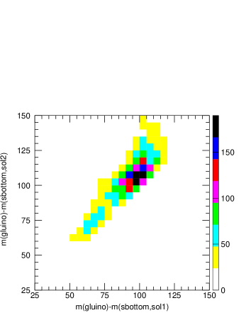
This formula is correct only at the endpoint of the three body decay $\tilde{\chi}^{0}_{2}\rightarrow\chi^{0}_{1}\ell\ell$, but is nevertheless approximately correct near the edge of $\tilde{\chi}^{0}_{2}\rightarrow\tilde{\ell}\ell\rightarrow\ell\ell\tilde{\chi}^{0}_{1}$ at SPS1a. The sbottom mass can then be calculated by building the invariant mass of the approximate $\tilde{\chi}^{0}_{2}$ obtained by using Eq. (12) with the leading $b$-jet in the event. The parton-level result is shown in Fig. 1(a), where we plot the difference between the reconstructed gluino mass and the reconstructed sbottom mass, to minimize the smearing introduced by the approximation of Eq. (12). The $\tilde{b}_{1}$ peak is reconstructed correctly. The bump on the left originates from the events from $\tilde{g}\rightarrow\tilde{b}_{2}$, and is centered on the position $m_{\tilde{g}}-m_{\tilde{b}_{2}}=$70.6 GeV. Even at parton level, with no experimental smearing the bump is not well separated from the $\tilde{b}_{1}$ peak at 103 GeV.

a)                                           b)

Figure 1: The distribution of $m_{\tilde{g}}-m_{\tilde{b}}$ calculated using a) parton level $b$ momentum and using the approximate relation Eq. (12) and b) by solving Eq. (6). For a) $m_{\ell\ell}>65$ GeV is required. For b), the two $m_{\tilde{b}}$ solutions for the input gluino mass of $m_{\tilde{g}}=595$ GeV are plotted in a two-dimensional plane, for both correct and wrong lepton assignment.

Unlike the relation Eq. (12), the formula Eq. (11) is exact. For each event we have in this case two possible lepton assignments, and for each lepton assignment, given an input value for the gluino mass, two solutions for the sbottom mass from the quadratic equation Eq. (11). We show in Fig. 1 the smaller solution versus the larger one of Eq. (11) for both of the lepton assignments. For the gluino mass the nominal value is assumed. Unlike in Fig. 1 a) two peaks of $\tilde{b}_{1}$ and $\tilde{b}_{2}$ are clearly separated in the plot. Furthermore the number of the available events for the mass fit are now increased by factor of 2 compared to the endpoint analysis because there are no constraint on the value of $m_{\ell\ell}$ when using Eq. (11).

The advantage of switching to the exact solution for the event kinematics is clearly demonstrated by the plots. In order to evaluate if the heavier sbottom state will be detectable we need to perform the study taking into account the smearing induced by the fact that $b$-jets rather than partons are measured in the detector.

V Event pair analysis

As discussed in section III, each event can be represented as a quadratic equation in the $m_{\tilde{g}}^{2}$, $m_{\tilde{b}}^{2}$ variables. By taking two events, we have a system of two equations in two unknowns which can be solved analytically. This yields up to four values for the squark and gluino masses. In the following, We start from the selected $bb\ell\ell$ events, and we build all the possible event pairs. In order to minimize the combinatorial backgrounds we use the pairings which satisfy the following conditions :

• Eq. (11) has solution for only one of the two possible lepton assignments.

• For the selected lepton assignment the resulting quartic equation in $m_{\tilde{g}}^{2}$ has only two solutions, and the difference of the gluino masses for the two solutions is more than 100 GeV. The smaller gluino mass solution is chosen.

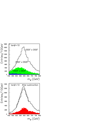
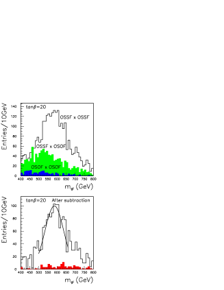
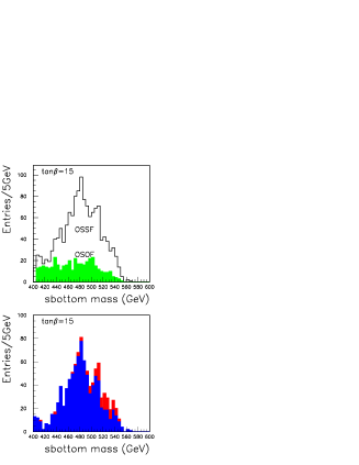
The $m_{\tilde{g}}$ distributions for the OSSF$\times$OSSF events pairs are shown in the histograms on the upper line of Fig. 2. A significant SUSY background, also shown in Fig. 2 is still present in the sample. This background can be estimated from the data themselves by using the $bb\ell\ell$ events with an opposite sign opposite flavor (OSOF) lepton pair (i.e. $\ell\ell=e^{\pm}\mu^{\mp}$). To this purpose we produce mass distributions for the three types of event pairs:

1. two OSSF lepton events (OSSF$\times$OSSF),

2. an OSSF lepton event and an OSOF lepton event (OSSF$\times$OSOF),

3. two OSOF lepton events (OSOF$\times$OSOF).

The background-subtracted distribution can be then obtained as the combination of the three distributions: OSSF$\times$OSSF$-$OSSF$\times$OSOF$+$OSOF$\times$OSOF.

The total number of event pairs is of course much larger than the number of events. Due to the selection criteria imposed to minimize the combinatorial backgrounds, some of the events are not used at all to make event pairs, while events which are used at least once are used O(10) times on average. The three histograms show peaks corresponding to the input value for the gluino mass even before the background subtraction. The green and blue histograms show the OSSF$\times$OSOF and OSOF$\times$OSOF distributions, respectively. The distributions after the background subtraction are shown in the histograms on the lower line of Fig. 2. The peak position and its error obtained by a Gaussian fit to the distribution are listed in Table 3. We also show in the histogram the gluino mass distribution for event pairs where at least one of the events comes from $\tilde{b}_{2}$ decay. The $\tilde{b}_{2}$ contribution is significantly smaller compared with the distribution of $\tilde{b}_{1}$ pair and does not affect the gluino mass fit. One can also look into the distribution of $m_{\tilde{g}}-m_{\tilde{b}}$ and estimating the value of this observable by performing a Gaussian fit on the observed peak. The result of the fit is also shown in Table 3.

The statistical error of the gluino mass measurement can be evaluated by performing the analysis on a set of statistically independent experiments. To perform the evaluation within a reasonable CPU budget, we generated a set of events where the $\tilde{b}_{1}$ is forced to decay with 100% BR into the desired decay chain, for the SPS1a Point ($\tan\beta=10$). The generated statistics corresponds to 30 experiments with an integrated luminosity of 300 fb^-1 each. By performing the analysis on the 30 experiments, we find that the spread for the measured gluino mass is 1.6 GeV for the benchmark integrated luminosity of 300 fb^-1. By construction, the presence of the combinatorial background is not considered in the error analysis. No large degradation of the resolution is expected once this effect is correctly taken into account.

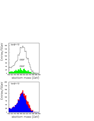
Once the gluino mass is fixed by the analysis shown above, Eq. (11) can be solved for each event for the sbottom mass, giving as input the central measured value for the gluino mass. Following this procedure, in Fig.  3, we plot the distribution of the smaller sbottom mass solution $m_{\tilde{b}}$(min) for both OSSF (signal) and OSOF (background) lepton pair events (top histograms). We show in the bottom line the mass distributions after the background subtraction, where the red regions show the contribution of $\tilde{b}_{2}$. The peak positions are evaluated by a Gaussian fit, and listed in Table 4. Note that the total number of the signal $\tilde{b}_{1}$ event is smaller by factor of 4 for $\tan\beta=20$ compared with $\tan\beta=10$, but the mass peak is seen very clearly. The $m_{\tilde{b}}$(min) peak and $m_{\tilde{b}}$(input) are in good agreement, and it is not so for the larger solution $m_{\tilde{b}}$(max).

The peak positions of the distribution of the events originated from $\tilde{b}_{2}$ decay are also consistent with $\tilde{b}_{2}$ masses. It is however evident from the plots that in the real experiment it will not be possible to claim the presence of the second peak. The existence of $\tilde{b}_{2}$ can be established only after understanding $b$-jet smearing and $\tilde{b}_{1}$ distribution correctly.

Figure 2: The gluino mass distributions for $\tan\beta=10$ (left), $\tan\beta=15$ (center) and $\tan\beta=20$ (right) with the event pair analysis. The open, green, and blue histograms in the top figures are for OSSF$\times$OSSF, OSSF$\times$OSOF, and OSOF$\times$OSOF event pairs, respectively. The open histograms in the bottom figures shows the mass distributions after background subtraction. The contributions of $\tilde{b}_{2}$ are shown by red histograms.

	$\tan\beta=10$	$\tan\beta=15$	$\tan\beta=20$
$m_{\tilde{g}}$	591.9	593.1	585.1
$m_{\tilde{g}}-m_{\tilde{b}}$	98.9	105.1	111.6

Table 3: Fit results of the gluino and and sbottom masses in the event pair analysis.

	$\tan\beta=10$	$\tan\beta=15$	$\tan\beta=20$
$m_{\tilde{b}}$(true)	491	485.3	478.8
$m_{\tilde{b}}$(min)	492.1$\pm$ 1.2	487.7$\pm$ 2.2	474.3$\pm$ 2.4
$m_{\tilde{b}}$(max)	504.5$\pm$ 1.0	502.9$\pm$ 1.7	495.1$\pm$ 2.4

Table 4: Fit results of the sbottom mass with a fixed gluino mass ($m_{\tilde{g}}=595$ GeV).

Figure 3: The $m_{\tilde{b}}$ distributions for $\tan\beta=10$ (left), 15 (center) and 20 (right) with a fixed gluino mass ($m_{\tilde{g}}=595$ GeV). The open and green histograms in the top figures show the distributions of OSSF and OSOF lepton events, respectively. The mass distributions after background subtraction are shown in the bottom figures, where the contribution of the $\tilde{b}_{2}$ events are shown by the red regions.

VI Likelihood analysis

The analysis shown in the previous section only uses the events in pairs to evaluate the values of the squark and gluino masses. A more efficient use of the available event statistics can be achieved by using all of the events at the same time and finding the ($m_{\tilde{g}},m_{\tilde{b}}$) pair for which the combined probability of all events is highest. We define in this section an approximate likelihood function for ($m_{\tilde{g}},m_{\tilde{b}}$), and we then apply it to detection of $\tilde{b}_{2}$.

VI.1 Construction of the likelihood function

From Eq. (11), each event is represented as a curve in the ($m_{\tilde{g}},m_{\tilde{b}}$) plane. The coefficients of the curve are a function of the four momenta of the detected partons. The partons are measured as jets in the detector, which smears the parton according to a smearing function. It depends on the detector performance and on the algorithms used to cluster the energy deposition in the detector.

Due to these experimental effects, in a frequentist approach, from the measured quadratic form for an event we can build a confidence belt in the ($m_{\tilde{g}},m_{\tilde{b}}$) plane. This should be built using a Neyman construction Hagiwara:2002fs , from the probability distribution for the measured values of ($m_{\tilde{g}},m_{\tilde{b}}$) as a function of the input values for the same two variables. In order to build this function, the crucial ingredient is the distribution of the measured $b$-jet momenta as a function of the $b$-parton momenta. Evaluating this distribution is outside the scope of this work, as it requires a detailed simulation of the detector response, which will need to be validated on real data using calibration samples of $b$-jets in the detector. Even assuming an approximate form for the $b$-jet response, the proper Neyman construction for each event is a very computing-intensive calculation.

We recast equation Eq. (11) in the form

$$f(m_{\tilde{g}},m_{\tilde{b}},p_{1},p_{2})=0$$

where $p_{1}$ and $p_{2}$ are the momenta of the two $b$-jets. We build an approximate probability density function according to the formula:

$${\cal L}(m_{\tilde{g}},m_{\tilde{b}})=\int dp^{\prime}_{1}\int dp^{\prime}_{2}\epsilon(p_{1}:p^{\prime}_{1})\epsilon(p_{2}:p^{\prime}_{2})\delta(f(m_{\tilde{g}},m_{\tilde{b}},p^{\prime}_{1},p^{\prime}_{2}))$$ (13)

where $\epsilon(p:p^{\prime})$ is the probability to measure a momentum $p^{\prime}$ for a $b$-jet, given a $b$-parton with momentum $p$.

In the equation we did not include the possibility of lepton momentum mis-measurement, which has an almost negligible effect, as compared to the smearing of $b$-partons. As a further simplification, we assume that the jet direction is not modified by the measurement and we use for $\epsilon(p:p^{\prime})$ a gaussian distribution, with a width $\sigma$ corresponding to the parameterized jet smearing used in the fast simulation program.

$$\sigma/E = 0.5/\sqrt{E{\rm(GeV)}}+0.03\ \ \ (|\eta|<3.0)$$ (14)

$$\sigma/E = 1.0/\sqrt{E{\rm(GeV)}}+0.07\ \ \ (|\eta|>3.0)$$ (15)

The gaussian smearing is not very good approximation for for $b$-jets for which in many cases the semi-leptonic decay of the $b$-quark results in jets containing an unmeasured neutrino. The approximate function takes however into account the dominant part of the jet smearing and can be used to demonstrate the method. Note also that in Eq. 13, we define our ${\cal L}$ using $\epsilon(p_{1},p_{1}^{\prime})$ where $p_{1}$ is measured $b$-jet momentum. The function ${\cal L}$ would correspond to the actual probability function only if the jet response were gaussian. A detailed experimental simulation will be needed in order to assess the validity of the obtained results in the real experimental situation.

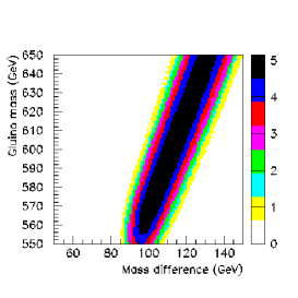
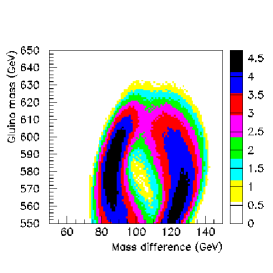
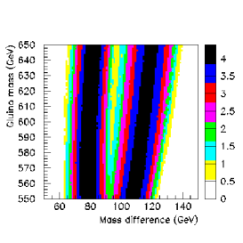
We now show $\log{\cal L}$ in the $(m_{\tilde{g}}-m_{\tilde{b}},m_{\tilde{g}})$ plane for a few events where the $bb\ell\ell$ events originates from the cascade decay of Eq. (1) at SPS1a. We calculate $\cal{L}$ using the following procedure. For each event in our sample, characterized by a ($p_{1},p_{2}$) pair of measured momenta for the $b$-jets, we generate Monte Carlo events where the two $b$-jets have momenta ($p^{\prime}_{1}$, $p^{\prime}_{2}$), where $p^{\prime}_{1}$ and $p^{\prime}_{2}$ are randomly generated according to the function $\epsilon(p_{1}:p^{\prime}_{1})\times\epsilon(p_{2}:p^{\prime}_{2})$. Each generated event corresponds to a curve in the ($m_{\tilde{g}}$, $m_{\tilde{b}}$) plane which satisfies the equation $f(m_{\tilde{g}},m_{\tilde{b}},p_{1},p_{2})=0$. We histogram of the number of curves that go through each bin of a $1\times 1$ GeV grid in the $(m_{\tilde{g}},m_{\tilde{b}})$ plane, for $n$ Monte Carlo events, normalized by dividing the bin contents by $n$. In the limit $n\rightarrow\infty$, this corresponds to

$${\cal L}(m_{\tilde{g}},m_{\tilde{g}}+\Delta m_{\tilde{g}};m_{\tilde{b}},m_{\tilde{b}}+\Delta m_{\tilde{b}})=\int Dp^{\prime}_{1}\int Dp^{\prime}_{2}\epsilon(p_{1}:p^{\prime}_{1})\epsilon(p_{2}:p^{\prime}_{2})\theta(p^{\prime}_{1},p^{\prime}_{2},m_{\tilde{g}},m_{\tilde{g}}+\Delta m_{\tilde{g}};m_{\tilde{b}},m_{\tilde{b}}+\Delta m_{\tilde{b}})$$ (16)

where $\theta(p^{\prime}_{1},p^{\prime}_{2},m_{\tilde{g}},m_{\tilde{g}}+\Delta m_{\tilde{g}};m_{\tilde{b}},m_{\tilde{b}}+\Delta m_{\tilde{b}})$ is 1 when the solution of Eq. (11) for the two $b$-jet momenta $p_{1}^{\prime}$ and $p_{2}^{\prime}$ goes through $(m_{\tilde{g}},m_{\tilde{g}}+\Delta m_{\tilde{g}};m_{\tilde{b}},m_{\tilde{b}}+\Delta m_{\tilde{b}})$ and otherwise 0. We take $n=10000$ for our calculations.

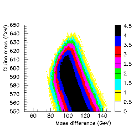
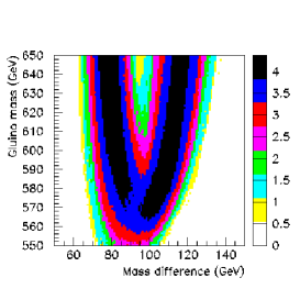
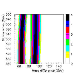
In Fig. 4, we plot

$$\Delta\log{\cal L}=\log({\cal L}(m_{\tilde{g}},m_{\tilde{g}}+\Delta m_{\tilde{g}},m_{\tilde{b}},m_{\tilde{b}}+\Delta m_{\tilde{b}})+c)-\log({\cal L}({\rm min})).$$ (17)

where $c=0.001$ is a constant cutoff factor, which is needed as for each event we generate only a finite number of Monte Carlo experiments, and therefore some bins can have zero hits. The shape of the probability density distribution is different event by event, as it depends on the event kinematics. For a few events the density distribution is parallel to the $y$ axis, therefore it only has sensitivity to the $m_{\tilde{g}}-m_{\tilde{b}}$ difference, but little sensitivity to the absolute value of the gluino mass. The size of the band with significant probability is also different event by event, which means that some events will have more weight in the determination of the mass parameters.

a)                                           b)                                            c)

d)                                           e)                                            f)

Figure 4: Likelihood distributions in the $(m_{\tilde{g}}-m_{\tilde{b}},m_{\tilde{g}})$ for selected events.

For each event, one defines in this way curves of equal probability in the ($m_{\tilde{g}},m_{\tilde{b}}$) plane. By combining the probabilities for different events, a region of maximum probability in the ($m_{\tilde{g}},m_{\tilde{b}}$) is found, where the curves of maximum probability for all events approximately cross. Given the fact that the curves have different shapes for different events, the region thus defined has a limited size, for an adequate number of events. This region can be taken as a measurement for $m_{\tilde{g}}$ and $m_{\tilde{b}}$. We perform the combination as the product of ${\cal L}$ for the all events, and we define

$$\log{\cal L}_{\rm comb}(m_{\tilde{g}},m_{\tilde{b}})\equiv\sum_{\rm events}\log{\cal L}(m_{\tilde{g}},m_{\tilde{b}})$$ (18)

As an estimator of the probability for a given ($m_{\tilde{g}},m_{\tilde{b}}$) pair, one can use

$$\Delta\chi^{2}(m_{\tilde{g}},m_{\tilde{b}})\sim\Delta\log{\cal L}\equiv\log{\cal L}_{\rm max}-\log{\cal L}_{\rm comb}(m_{\tilde{g}},m_{\tilde{b}})$$ (19)

Given the approximations introduced this does not however correspond to the statistical definition of $\Delta\chi^{2}$.

VI.2 Event analysis

By following the procedure described in the previous subsection we can build the combined likelihood for all the events defined as:

$$\log{\cal L}_{\rm comb}(m_{\tilde{g}},m_{\tilde{g}}+\Delta m_{\tilde{g}},m_{\tilde{b}},m_{\tilde{b}}+\Delta m_{\tilde{b}})=\sum_{\rm events}\log({\cal L}(m_{\tilde{g}},m_{\tilde{g}}+\Delta m_{\tilde{g}},m_{\tilde{b}},m_{\tilde{b}}+\Delta m_{\tilde{b}})+c).$$ (20)

As in Eq. (17) we have introduced a constant cutoff parameter $c=0.001$ and the number of Monte Carlo experiments used to build the likelihood for each event $n=10000$.

As we can see in Fig. 2, there are significant backgrounds from accidental leptons. The background subtraction must be carried out using events with OSOF lepton pairs. The correct log likelihood function is schematically expressed as

$$\log{\cal L}_{\rm total}({\bf m}_{\tilde{g}},{\bf m}_{\tilde{b}},.....)=\sum_{\rm OSSF}\log{\cal L}({\bf m}_{\rm sig},{\bf m}_{\rm bg})+\sum_{\rm OSOF}{\cal L}({\bf m}_{\rm bg})$$ (21)

where ${\bf m}_{\rm sig}$ express the parameters relevant to the signal distribution, such as the masses of the sparticles involved in the cascade decay, the decay branching ratios and so on. On the other hand ${\bf m}_{\rm bg}$ are all the other parameters relevant to the OSSF and OSOF events. This is rather complex procedure which is out of the scope of this paper. Instead, we take the difference of the functions for OSSF and OSOF lepton pair events

$$\log{\cal L}_{\rm sub}\equiv\log{\cal L}_{\rm OSSF}-\log{\cal L}_{\rm OSOF}\equiv\sum_{\rm OSSF}\log{\cal L}-\sum_{\rm OSOF}\log{\cal L}.$$ (22)

In the limit of infinite statistics, $\log{\cal L}_{\rm sub}$ should be independent from the contribution of accidental lepton pairs. Therefore we use $\log{\cal L}_{\rm sub}$ in this paper.

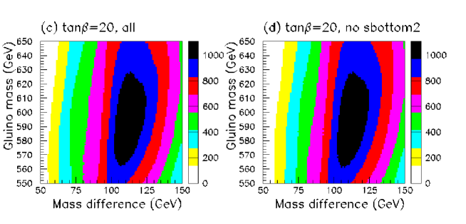
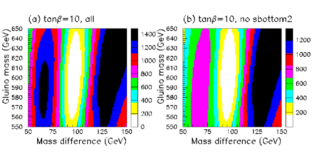
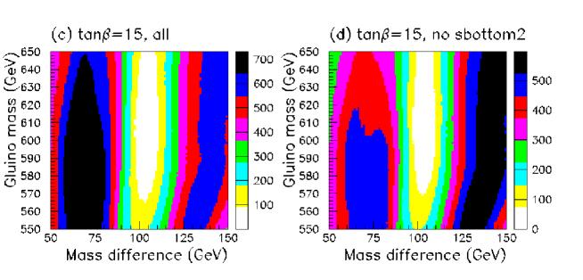
We plot the contours of the function $\log{\cal L}_{\rm sub}$ in Fig. 5, where plots (a) and (b) [(c) and (d)] are for $\tan\beta=10$ [$\tan\beta=20$]. The distributions (a) and (c) are produced accepting all the events which pass the selections, whereas distributions (b) and (d) are produced using an event sample where the events including a $\tilde{b}_{2}$ decay have been rejected.

In Fig. 5 (a) and (c), the position of the peak for $m_{\tilde{g}}-m_{\tilde{b}}$ is roughly consistent with the input value. Unlike the gluino and sbottom mass fits in the previous section, we obtain the correct peak position without the need of artificially choosing among multiple solutions. The likelihood distribution can be used to determine the $\tilde{g}$ and $\tilde{b}$. We restrict the likelihood distribution for $591$ GeV $<m_{\tilde{g}}<599$ GeV(within 4 GeV from the input gluino mass). We then fit the distribution around the peak assuming gaussian distribution, The likelihood distribution peaks at the gluino and sbottom mass difference as 99.5 GeV for $\tan\beta=10$, 104.2 GeV for $\tan\beta=15$, and 113.9 GeV for $\tan\beta=20$, where the input value is 103.3 GeV, 109.9 GeV and 116.5 GeV, respectively. The fitted values display shift of about 4 GeV from the true value. We ascribe this effect to our simplified modeling of the jet smearing in building the likelihood function, which should disappear once the detector response is properly taken into account in the unfolding procedure.

By comparing the left side with the right side of Fig 5, we also observe a slight shift in the position of the maxima of the distributions, showing that the distributions are sensitive to the presence of $\tilde{b}_{2}$ decays. The $\tilde{b}_{2}$ contribution however manifests itself in Fig. 5 (a) and (c) only as a flattening of the distribution around $m_{\tilde{g}}-m_{\tilde{b}}=70$ GeV at $m_{\tilde{g}}\sim 595$ GeV. No secondary peak can be observed because of the experimental smearing, and of the fact that the branching ratio into $\tilde{b}_{2}$ is much smaller.

Figure 5: Contours of the likelihood function $\log{\cal L}_{\rm sub}$ in the $(m_{\tilde{g}}-m_{\tilde{b}},m_{\tilde{g}})$ plane: (a) and (b) for $\tan\beta=10$ and (c) and (d) for $\tan\beta=20$, respectively. The contours (b) and (d) are made without $\tilde{b}_{2}$ contributions.

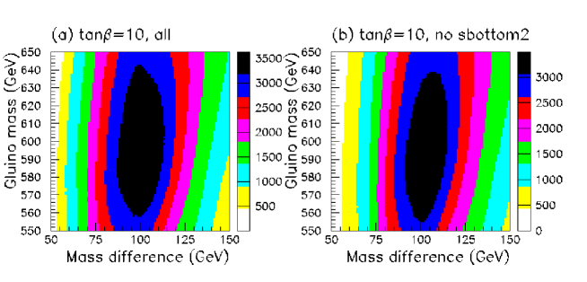
In Fig. 6(a), we show the distribution of $\log{\cal L}_{\rm sub}$ as a function of $m_{\tilde{g}}-m_{\tilde{b}}$ at $\tan\beta=20$, restricting the gluino mass in the region $591$ GeV$<m_{\tilde{g}}<$599 GeV again. On the left of the peak corresponding to the $\tilde{b}_{1}$ mass, we see a small bump in the distribution. This bump is not observed in the mass distribution made without $\tilde{b}_{2}$ contribution (Fig. 6(b)). In order to claim the presence of a second component in the distribution on the data, the ability of correctly reproducing the likelihood distribution for $\tilde{b}_{1}$ events would be needed. It is also difficult to extract a statistical significance for the $\tilde{b}_{2}$ shoulder as our definition of the likelihood function is approximate one, and we did not treated the background subtraction correctly as can be seen in Eq. (22).

In Fig. 3, it is rather hard to see the effect of $\tilde{b}_{2}$ unlike in Fig. 6. The apparent discrepancy probably comes from the fact that the likelihood analysis is more sensitive to the model parameter than simply solving Eq. (11) for a fixed gluino mass. The likelihood analysis not only takes care of the most plausible value of the sbottom mass for a fixed gluino mass, but also includes possible statistical fluctuations, which vary event by event as seen in Fig. 4. For example, badly mis-measured events have less chance to be consistent with the input gluino mass, providing a natural cut for the event selection.

Figure 6: The likelihood as a function of $m_{\tilde{g}}-m_{\tilde{b}}$ for $\tan\beta=20$: (a) for all events and (b) without $\tilde{b}_{2}$ events.

A significant part of the background under the $\tilde{b}_{2}$ is the tail of the smeared probability distribution for events which correctly reconstruct the $\tilde{b}_{1}$ mass. One can therefore try to remove from the distributions the events consistent with $\tilde{b}_{1}$ in order to improve the signal to background ratio for $\tilde{b}_{2}$. To reduce the $\tilde{b}_{1}$ events, an event is required to satisfy the condition

$$\sum_{\rm cut\ region}{\cal L}<{\cal L}_{\rm cut}\,$$ (23)

where the sum is made for bins in a cut region in the $({m_{\tilde{g}}-m_{\tilde{b}},m_{\tilde{g}}})$ plane. We choose the region as $550$ GeV$<m_{\tilde{g}}<$ $650$ GeV, and $m({\rm min})$ $<m_{\tilde{g}}-m_{\tilde{b}}<$ $m({\rm max})$, which corresponds to the region around the $\tilde{b}_{1}$ peak. We use the cut value ${\cal L}_{\rm cut}=20$. The relevant $m({\rm min})$ and $m({\rm max})$ values are listed in Table 5. The contours of $\log{\cal L}_{\rm sub}$ after this cut are shown in Fig. 7: (a) and (b) for $\tan\beta=10$ and (c) and (d) for $\tan\beta=15$. The contours (b) and (d) are made without the $\tilde{b}_{2}$ contribution. By comparing the contours with and without the $\tilde{b}_{2}$ contribution, the presence of the $\tilde{b}_{2}$ can be clearly observed in the plots. In Fig. 8, we again plot the likelihood function as the function of $m_{\tilde{g}}-m_{\tilde{b}}$, for $550$ GeV$<m_{\tilde{g}}<$ $650$ GeV. The distributions without the $\tilde{b}_{2}$ contribution are also shown as dashed histograms. The signal to background ratio is much improved with respect to what is seen on the left side of Fig. 6, and it is about 1:1. However, from an inspection of the mass distribution event by event, the purity of the signal after the likelihood cut does not appear significantly improved with respect to Fig. 3. Moreover the position of the peak corresponding to $\tilde{b}_{2}$ is dependent from the cuts applied. This is illustrated in Table 5, where the results of fits to the peak position are shown for two different values of the applied cuts both for the full sample and for the pure $\tilde{b}_{2}$ signal. Even when only considering the $\tilde{b}_{2}$ signal, the peak position depends on the cuts, albeit with a milder dependence than for the full sample. It will therefore be problematic to extract a mass measurement from Fig. 8, even assuming a priori the existence of a $\tilde{b}_{2}$ contribution.

Figure 7: The contours of the likelihood function in the $(m_{\tilde{g}}-m_{\tilde{b}}$, $m_{\tilde{g}})$ plane after the cut given in Eq. (23): (a) and (b) are with and without $\tilde{b}_{2}$ events at $\tan\beta=10$, respectively, and (c) and (d) at $\tan\beta=15$.

Figure 8: The likelihood as a function of $m_{\tilde{g}}-m_{\tilde{b}}$ with the cut given in Eq. (23): (left) for $\tan\beta=10$ and (right) for $\tan\beta=15$.

	$m$(min)	$m$(max)	all	$\tilde{b}_{2}$ only
$\tan\beta=10$	87	108	64.1 $\pm$ 0.2	62.7 $\pm$ 0.3
	82	113	60.3 $\pm$ 0.3	60.2 $\pm$ 0.5
$\tan\beta=15$	94	115	61.1 $\pm$ 0.7	65.3 $\pm$ 0.4
	89	120	62.7 $\pm$ 0.3	62.6 $\pm$ 0.6

Table 5: The peak positions at the smaller $m_{\tilde{g}}-m_{\tilde{b}}$ region in Fig. 8 for $\tan\beta=10$ and 15. The peak positions for the signal $\tilde{b}_{2}$ distribution are also shown.

VII Discussion

Supersymmetric models predict the existence of heavy superpartners which decay subsequently into the lighter superpartners. The lightest SUSY particle is stable and neutral, and escapes detection. Therefore two undetected particles will be present in each event. Moreover the partonic center of mass energy is unknown for hadron collisions. As a result, the complete kinematic reconstruction of SUSY events at hadron colliders is problematic.

We propose a new analysis method to solve the decay kinematics of this decay at the LHC, based on imposing the on-shell condition on the momenta of the particles participating in the cascade. The single cascade decay is solvable if a decay chain consisting of at least 4 successive two-body decays, involving 5 sparticles can be identified. In this case each event defines the 4 dim hypersurface in the 5 dim sparticle mass space. The potential of this method should be compared to the method previously used for this analysis based on the measurement of kinematic edges of invariant mass combinations of the detected decay particles.

The merits and demerits of the new method may be summarized as follows:

• The cascade decay is solved based on the exact formulae.

• Mass peaks would be reconstructed, as opposed to the kinematic edges. This allows us to perform measurements even if the significant backgrounds exist or statistics are small. Note that backgrounds will not exhibit peaks corresponding to the signal region.

• In the case where sfermion masses are heavier than gaugino masses, the cascade decays are expected to be shorter, and one can not therefore use this method. The endpoint method provides a mass information even in this case.

We note that in case two decay chains can be simultaneously identified in the event, the method can be applied to shorter decay chains, consisting of only three decays each. In fact in this case two additional constraints can be applied by requiring that the sums of the transverse components of the momenta of the two lightest neutralinos equal the two components of the measured missing transverse momentum.

Further on, if one sparticle cascade decay is solved by the mass relation method, the candidate LSP momentum $p_{T}$ would be obtained. We can then calculate the transverse momentum of the other LSP $p^{\prime}_{T}$ as:

$$p^{\prime}_{T}=-p_{T}+P_{\rm miss}.$$ (24)

For the cascade decay to which the second LSP belongs only two components of the neutralino four momentum are unknown, therefore a cascade decay with $n_{decay}\geq 3$ can be solved.

To see the performance of the mass relation method, we have studied in this paper the problem of measuring sparticle masses in the cascade decay: $\tilde{g}\rightarrow\tilde{b}b_{2}\rightarrow\tilde{\chi}^{0}_{2}b_{1}b_{2}\rightarrow\tilde{\ell}b_{1}b_{2}\ell_{2}\rightarrow\tilde{\chi}^{0}_{1}b_{1}b_{2}\ell_{1}\ell_{2}$. We have performed a detailed study for some benchmark SUSY model points including backgrounds and a parameterized simulation of detector effects. We performed the exercise in a simplified fashion, by fixing the masses of the three lighter particles to avoid the practical complications in handling a large number of parameters. Then each event becomes an allowed curve in the gluino-sbottom mass plane, passing through the point corresponding to the true gluino and sbottom masses. We first addressed the mass reconstruction through the “event pair analysis”, which determines the sparticle masses from the distribution of the solutions of any event pairs in the selected sample. The method reconstructs $m_{\tilde{b}_{1}}$ correctly for SPS1a where $\tan\beta$ is varied from 10 to 20. Note that the signal branching ratio becomes a factor 4 smaller for $\tan\beta=20$ with respect to $\tan\beta=10$, but the $\tilde{b}_{1}$ peak is still clearly observable. On the other hand, in order to obtain the correct mass, one needs to artificially choose among the multiple available solutions.

A more global approach requires the usage of all available events simultaneously. For this approach we constructed an approximate likelihood function for the true gluino and sbottom masses, taking into account the experimental smearing in the measurement of the $b$-jets. When the peak position of the likelihood distribution is used to extract the mass, the $\tilde{b}_{1}$ mass is measured without the problem of the multiple solutions of the event pair analysis.

We also try to probe the presence of a $\tilde{b}_{2}$ in our Monte Carlo sample. The sbottom mass matrix is parameterized by three parameters $m_{\tilde{b}_{1}}$, $m_{\tilde{b}_{2}}$ and the mixing angle $\theta$. Successful extraction of the $\tilde{b}_{2}$ would be an important step to fully understand the nature of the third generation sparticles. No clear result is achieved for $\tilde{b}_{2}$, as the branching ratio into $\tilde{b}_{2}$ is small for the parameters we have chosen, and also the small difference between the two sbottom states is comparable to the resolution in the experimental measurement of jet momenta. It is however clear that, even with the small statistics available for the case $\tan\beta=20$, a hint for the deviation from a single-mass case can be seen in the distribution.

The physics output of our analysis is therefore the possibility to extract information on the third generation sector, even for rather small input statistics. The measurement of the third generation sparticle masses are important theoretically. In mSUGRA, $\tilde{b}_{L(R)}$ masses are same as the other sparticle masses at the GUT scale but non-universality is induced by RGE running at the weak scale due to the Yukawa coupling. In addition to that, the left-right mixing of sbottom is induced by the $F$ term of the Superpotential which is proportional to $\mu\tan\beta$. The mass shift around 20 GeV from $\tan\beta=10$ and $\tan\beta=20$ is due to the mixing effect. Our method is sensitive to the $\tan\beta$ dependence as it could yield a sensitivity to the mass difference between the two states of the order of a few GeV.

Appendix

As described in section 2, we have solved the cascade decay in Eq. (1) by expanding the the lightest neutralino momentum by the momenta of $l_{1}$, $l_{2}$ and $b_{1}$ as in Eq. (7)

$$\vec{\rm p}_{\tilde{\chi}^{0}_{1}}=a\vec{\rm p}_{\ell_{1}}+b\vec{\rm p}_{\ell_{2}}+c\vec{\rm p}_{b_{1}}$$

The parameters $(a,b,c)$ may be written as the function of sparticle masses and the LSP energy as:

$$\left(\begin{array}[]{c}a\cr b\cr c\cr\end{array}\right)={\cal M}^{-1}\left[[{{\rm x_{1}}}]m_{\tilde{\chi}^{0}_{1}}^{2}+[{{\rm x_{2}}}]m_{\tilde{b}}^{2}+[{{\rm x_{3}}}]m_{\tilde{\chi}^{0}_{1}}E_{\tilde{\chi}^{0}_{1}}\right]={\cal M}^{-1}{\cal X}\left(\begin{array}[]{c}m_{\tilde{\chi}^{0}_{1}}^{2}\cr m_{\tilde{b}}^{2}\cr m_{\tilde{\chi}^{0}_{1}}E_{\tilde{\chi}^{0}_{1}}\end{array}\right),$$ (25)

where

$${\cal X} = [{\rm x_{1}},{\rm x_{2}},{\rm x_{3}}],$$ (26)

$$[{\rm x_{1}}] = \frac{1}{2m^{2}_{\tilde{\chi}^{0}_{1}}}\left(\begin{array}[]{l}-m_{\tilde{\ell}}^{2}+m_{\tilde{\chi}^{0}_{1}}^{2}\cr-m_{\tilde{\chi}^{0}_{2}}^{2}+m_{\tilde{\ell}}^{2}+2p_{\ell_{1}}\cdot p_{\ell_{2}}\cr m_{\tilde{\chi}^{0}_{2}}^{2}+m_{b}^{2}+2p_{b_{1}}\cdot(p_{\ell_{1}}+p_{\ell_{2}})\end{array}\right),$$ (30)

$$[{\rm x_{2}}] = \left(\begin{array}[]{c}0\cr 0\cr-1/2\end{array}\right),\ \ [{\rm x_{3}}]=\frac{1}{m_{\tilde{\chi}^{0}_{1}}}\left(\begin{array}[]{c}E_{\ell_{1}}\cr E_{\ell_{2}}\cr E_{b_{1}}\end{array}\right).$$ (37)

and $M$ is defined already in section 2 as:

$${\cal M}=\left(\begin{array}[]{ccc}\vec{\rm p}_{\ell_{1}}\cdot\vec{\rm p}_{\ell_{1}}&\vec{\rm p}_{\ell_{1}}\cdot\vec{\rm p}_{\ell_{2}}&\vec{\rm p}_{\ell_{1}}\cdot\vec{\rm p}_{b_{1}}\cr\vec{\rm p}_{\ell_{1}}\cdot\vec{\rm p}_{\ell_{2}}&\vec{\rm p}_{\ell_{2}}\cdot\vec{\rm p}_{\ell_{2}}&\vec{\rm p}_{\ell_{2}}\cdot\vec{\rm p}_{b_{1}}\cr\vec{\rm p}_{\ell_{1}}\cdot\vec{\rm p}_{b_{1}}&\vec{\rm p}_{\ell_{2}}\cdot\vec{\rm p}_{b_{1}}&\vec{\rm p}_{b_{1}}\cdot\vec{\rm p}_{b_{1}}\cr\end{array}\right).$$ (41)

By using the on-shell condition of the neutralino mass

$$E_{\tilde{\chi}^{0}_{1}}^{2}=(a,\ b,\ c){\cal M}\left(\begin{array}[]{c}a\cr b\cr c\end{array}\right)+m_{\tilde{\chi}^{0}_{1}}^{2},$$ (42)

we obtain the following equation:

$$A_{33}\left(\frac{E_{\tilde{\chi}^{0}_{1}}}{m_{\tilde{\chi}^{0}_{1}}}\right)^{2}+2\left(A_{13}+\frac{m_{\tilde{b}}^{2}}{m_{\tilde{\chi}^{0}_{1}}^{2}}A_{23}\right)\left(\frac{E_{\tilde{\chi}^{0}_{1}}}{m_{\tilde{\chi}^{0}_{1}}}\right)+\left(A_{11}+2\frac{m_{\tilde{b}}^{2}}{m_{\tilde{\chi}^{0}_{1}}^{2}}A_{12}+\frac{m_{\tilde{b}}^{4}}{m_{\tilde{\chi}^{0}_{1}}^{4}}A_{22}\right)=0,$$

where $A_{ij}=[{\rm x_{i}}]^{T}{\cal M}^{-1}[{\rm x_{j}}]-\delta_{ij}(i-2)/m_{\tilde{\chi}^{0}_{1}}^{2}$ The solution of $E_{\tilde{\chi}^{0}_{1}}$ is expressed as

$$E_{\tilde{\chi}^{0}_{1}} = \frac{m_{\tilde{\chi}^{0}_{1}}}{A_{33}}\left(-A_{13}-\frac{m_{\tilde{b}}^{2}}{m_{\tilde{\chi}^{0}_{1}}^{2}}A_{23}\pm\sqrt{D}\right),$$ (43)

$$D = \left(A_{13}+\frac{m_{\tilde{b}}^{2}}{m_{\tilde{\chi}^{0}_{1}}^{2}}A_{23}\right)^{2}-A_{33}\left(A_{11}+2\frac{m_{\tilde{b}}^{2}}{m_{\tilde{\chi}^{0}_{1}}^{2}}A_{12}+\frac{m_{\tilde{b}}^{4}}{m_{\tilde{\chi}^{0}_{1}}^{4}}A_{22}\right)$$ (45)

$$= \left(\frac{m_{\tilde{b}}^{2}}{m_{\tilde{\chi}^{0}_{1}}^{2}}\right)^{2}\left(A_{23}^{2}-A_{33}A_{22}\right)+2\left(\frac{m_{\tilde{b}}^{2}}{m_{\tilde{\chi}^{0}_{1}}^{2}}\right)\left(A_{13}A_{23}-A_{33}A_{12}\right)$$ (49)

$$+\left(A_{13}^{2}-A_{11}A_{33}\right).$$

When the sbottom comes from gluino decay, we can further use the gluino mass shell condition:

$$m_{\tilde{g}}^{2}=2p_{b_{2}}\cdot p_{\tilde{\chi}^{0}_{1}}+2p_{b_{2}}\cdot(p_{b_{1}}+p_{\ell_{2}}+p_{\ell_{1}})+m_{\tilde{b}}^{2}+m_{b}^{2},$$ (50)

where

$$p_{b_{2}}\cdot p_{\tilde{\chi}^{0}_{1}} = E_{\tilde{\chi}^{0}_{1}}E_{b_{2}}-\vec{\rm p}_{b_{2}}\cdot\vec{\rm p}_{\tilde{\chi}^{0}_{1}}=m_{\tilde{\chi}^{0}_{1}}^{2}F_{0}+F_{1}m_{\tilde{b}}^{2}+F_{2}m_{\tilde{\chi}^{0}_{1}}^{2}\left(\frac{\sqrt{D}}{A_{33}}\right),$$ (51)

$$F_{0} \equiv -\left(\frac{E_{b_{2}}}{m_{\tilde{\chi}^{0}_{1}}}-[{\cal K}_{b2}]^{T}\cdot[{\rm x_{3}}]\right)\left(\frac{A_{13}}{A_{33}}\right)-[{\cal K}_{b2}]^{T}[{\rm x_{1}}],$$ (52)

$$F_{1} \equiv -\left(\frac{E_{b_{2}}}{m_{\tilde{\chi}^{0}_{1}}}-[{\cal K}_{b2}]^{T}\cdot[{\rm x_{3}}]\right)\left(\frac{A_{23}}{A_{33}}\right)-[{\cal K}_{b2}]^{T}[{\rm x_{2}}],$$ (53)

$$F_{2} \equiv \pm\left(\frac{E_{b_{2}}}{m_{\tilde{\chi}^{0}_{1}}}-[{\cal K}_{b2}]^{T}\cdot[{\rm x_{3}}]\right),$$ (54)

$$[{\cal K}_{b2}]^{T} \equiv (\vec{\rm p}_{b_{2}}\cdot\vec{\rm p}_{\ell_{1}},\ \vec{\rm p}_{b_{2}}\cdot\vec{\rm p}_{\ell_{2}},\ \vec{\rm p}_{b_{2}}\cdot\vec{\rm p}_{b_{1}}){\cal M}^{-1}.$$ (55)

The equation involving the gluino and sbottom masses is of the form

$$Q_{11}m_{\tilde{g}}^{4}+2Q_{12}m_{\tilde{g}}^{2}m_{\tilde{b}}^{2}+Q_{22}m_{\tilde{b}}^{4}+2Q_{1}m_{\tilde{g}}^{2}+2Q_{2}m_{\tilde{b}}^{2}+Q=0,$$

where

$$Q_{11} = 1,\ \ Q_{12}=-2F_{1}-1,$$ (56)

$$Q_{22} = (2F_{1}+1)^{2}-F_{2}^{2}\frac{A_{23}^{2}-A_{33}A_{22}}{A^{2}_{33}},$$ (57)

$$Q_{1} = -2F_{0}m_{\tilde{\chi}^{0}_{1}}^{2}-2p_{b_{2}}\cdot(p_{b_{1}}+p_{\ell_{1}}+p_{\ell_{2}})-m_{b}^{2},$$ (58)

$$Q_{2} = Q_{12}Q_{1}-F_{2}^{2}m_{\tilde{\chi}^{0}_{1}}^{2}\frac{A_{13}A_{23}-A_{33}A_{12}}{A^{2}_{33}},$$ (59)

$$Q = Q_{1}^{2}-F_{2}^{2}m_{\tilde{\chi}^{0}_{1}}^{4}\frac{A_{13}^{2}-A_{11}A_{33}}{A^{2}_{33}}.$$ (60)

It should be noted that one can derive a equation of the form $m_{I}^{4}+C_{1}m_{I}^{2}+C_{2}=0$ for any particle $I$ involved in the cascade.

References

- (1) ATLAS Collaboration, ATLAS detector and physics performance Technical Design Report, CERN/LHCC 99-14/15 (1999).
- (2) S. Abdullin et al. [CMS Collaboration], J. Phys. G 28, 469 (2002) [arXiv:hep-ph/9806366].
- (3) I. Hinchliffe, F. E. Paige, M. D. Shapiro, J. Soderqvist and W. Yao, Phys. Rev. D 55, 5520 (1997) [arXiv:hep-ph/9610544].
- (4) I. Hinchliffe and F. E. Paige, Phys. Rev. D 61, 095011 (2000) [arXiv:hep-ph/9907519].
- (5) H. Bachacou, I. Hinchliffe and F. E. Paige, Phys. Rev. D 62, 015009 (2000) [arXiv:hep-ph/9907518].
- (6) B. C. Allanach, C. G. Lester, M. A. Parker and B. R. Webber, JHEP 0009, 004 (2000) [arXiv:hep-ph/0007009].
- (7) B.K. Gjelsten, E. Lytken, D.J. Miller, P. Osland, and G. Polesello, ATLAS internal note ATL-PHYS-2004-007.
- (8) M. M. Nojiri, D. Toya and T. Kobayashi, Phys. Rev. D 62 (2000) 075009 [arXiv:hep-ph/0001267].
- (9) M. M. Nojiri, G. Polesello and D. R. Tovey, arXiv:hep-ph/0312317.
- (10) C. Lester, in B. C. Allanach et al. [Beyond the Standard Model Working Group Collaboration], “Les Houches ’Physics at TeV Colliders 2003’ Beyond the Standard Model Working Group: Summary report,” arXiv:hep-ph/0402295.
- (11) B. C. Allanach et al., in Proc. of the APS/DPF/DPB Summer Study on the Future of Particle Physics (Snowmass 2001) ed. N. Graf, Eur. Phys. J. C 25 (2002) 113 [eConf C010630 (2001) P125] [arXiv:hep-ph/0202233].
- (12) H. Baer, F. E. Paige, S. D. Protopescu and X. Tata, arXiv:hep-ph/0312045.
- (13) G. Corcella et al., JHEP 0101, 010 (2001) [arXiv:hep-ph/0011363].
- (14) S. Moretti, K. Odagiri, P. Richardson, M. H. Seymour and B. R. Webber, JHEP 0204, 028 (2002) [arXiv:hep-ph/0204123].
- (15) E. Richter-Was, D. Froidevaux, and L. Piggishly, ATLAS internal note ATL-PHYS-98-131.
- (16) M. Chiorboli and A. Tricomi, CMS internal note CMS-RN 2003/002 (2003).
- (17) K. Hagiwara et al. [Particle Data Group Collaboration], Phys. Rev. D 66 (2002) 010001.