Effective Theory Approach to the Skyrme model
and Application to Pentaquarks

Abstract

The Skyrme model is reconsidered from an effective theory point of view. From the most general chiral Lagrangian up to including terms of order $p^{4}$, $N_{c}$ and $\delta m^{2}$ ($\delta m\equiv m_{s}-m$), new interactions, which have never been considered before, appear upon collective coordinate quantization. We obtain the parameter set best fitted to the observed low-lying baryon masses, by performing the second order perturbative calculations with respect to $\delta m$. We calculate the masses and the decay widths of the other members of (mainly) anti-decuplet pentaquark states. The formula for the decay widths is reconsidered and its baryon mass dependence is clarified.

I Introduction

Evidence of a new baryonic resonance state, called $\Theta^{+}(1540)$, has been claimed recently by Nakano et. al.Nakano:2003qx , with $S=+1$ and a very narrow width $\Gamma\leq 15$ MeV. Several other experimental groups have confirmed the existenceBarmin:2003vv ; Stepanyan:2003qr ; Barth:2003es . It appears in the recent version of Reviews of Particle PhysicsEidelman:2004wy with the *** rating, though its parity has not been established. Evidences of less certain exotic pentaquark states, $\phi(1860)$Alt:2003vb and $\Theta_{c}^{+}$Aktas:2004qf ; Chekanov:2004kn have also been claimed. The discovery of the pentaquarks is expected to lead us to a deeper understanding of strong interactions at low energies. In reality, it stimulates new ideas and reconsideration of old theories and experimental data.

The discovery was motivated by a paper by Diakonov, Petrov and PolyakovDiakonov:1997mm . They predicted the masses and the widths of the anti-decuplet, of which $\Theta^{+}$ is presumed to be a member, within the framework of the “chiral quark-soliton model”($\chi$QSM). See Ref. Diakonov:2000pa for a review of the $\chi$QSM. The chiral quark-soliton model prediction is reexamined in Refs. Praszalowicz:2003ik ; Ellis:2004uz . See also Refs. Manohar:1984ys ; Chemtob:1985ar ; Praszalowicz:1987em for earlier papers on the anti-decuplet in the Skyrme model.

Jaffe and WilczekJaffe:2003sg , on the other hand, proposed a quark model picture of pentaquarks based on diquark correlation. See Ref. Jaffe:2004ph for a review of this approach and other interesting aspects.

Since Witten pointed out that baryons may be considered as solitonsWitten:1979kh in the large-$N_{c}$ limit'tHooft:1973jz , and showed that the soliton (“Skyrmion”) has the right spin-statisticsWitten:1983tx thanks to the Wess-Zumino-Witten (WZW) termWess:1971yu ; Witten:1983tw , much effort has been done to explore the consequences. But the results do not look very successful. In order to fit the results to the observed values of masses, coupling constants, such as the pion decay constant, which appear in the chiral Lagrangian must be very different from the experimental values. For example, in the $SU(3)$ Skyrme model, the pion decay constant becomes typically one third of the experimental value to reproduce the correct mass splittingPraszalowicz:1985bt . It also predicted an anti-decupletManohar:1984ys ; Chemtob:1985ar ; Praszalowicz:1987em , which many did not believe to exist at that time.

But $\Theta^{+}$ has been discovered! It is time to take a serious look at the Skyrme model again.

One of the most important aspects of $\Theta^{+}$ is its narrowness. Several analyses of older data indicate that the width may be less than 1 MeVNussinov:2003ex ; Arndt:2003xz ; Workman:2004yd ; Cahn:2003wq . Interestingly, the Skyrme model is believed to be capable to explain the narrowness. It is claimed that the width becomes very narrow due to a strong cancellationPraszalowicz:2003tc .

A natural question is: Is this a general result of the Skyrme model, or a “model-dependent” one? What is the most general Skyrme model? The Skyrme model is nothing but a model. But, as Witten emphasized, the soliton picture of baryons is a general consequence of the large-$N_{c}$ limit of QCD. Assuming that the large-$N_{c}$ QCD bears a close resemblance to the real QCD, we may consider an effective theory (not just a model) of baryons based on the soliton picture, which may be called as the “Skyrme-Witten large-$N_{c}$ effective theory.”

Our key observation is that the Skyrme model conventionally starts with the particular chiral Lagrangian, which consists of the kinetic term, the Skyrme term (which stabilizes the soliton), the WZW term and the leading $SU(3)$ breaking term,

$$S_{Skyrme} = \frac{F_{\pi}^{2}}{16}\int d^{4}x\mbox{\rm Tr}\left(\partial_{\mu}U\partial^{\mu}U^{\dagger}\right)+\frac{1}{32e^{2}}\int d^{4}x\mbox{\rm Tr}\left(\left[U^{\dagger}\partial_{\mu}U,U^{\dagger}\partial_{\nu}U\right]^{2}\right)+N_{c}\Gamma[U]$$ (1)

$${}+\frac{F_{\pi}^{2}B}{8}\int d^{4}x\mbox{\rm Tr}\left({\cal M}^{\dagger}U+{\cal M}U^{\dagger}\right),$$

where ${\cal M}$ is the quark mass matrix

$${\cal M}=\left(\begin{array}[]{ccc}m&0&0\\ 0&m&0\\ 0&0&m_{s}\end{array}\right).$$ (2)

and

$$\Gamma[U]=\frac{i}{240\pi^{2}}\int_{Q}d\Sigma^{ijklm}\mbox{\rm Tr}\bigg{[}\left(\partial_{i}U\right)U^{\dagger}\left(\partial_{j}U\right)U^{\dagger}\left(\partial_{k}U\right)U^{\dagger}\left(\partial_{l}U\right)U^{\dagger}\left(\partial_{m}U\right)U^{\dagger}\bigg{]}$$ (3)

is the WZW term. The chiral perturbation theoryGasser:1983yg ; Gasser:1984gg ($\chi$PT) is however an effective field theory with infinitely many operators. We should keep it in mind that there are (infinitely) many other terms and the expansion must be systematic.

In this paper, we explore such an “effective theory” approach, i.e., an approach based on a systematic expansion of the operators based on the symmetry and power-counting. The parameters are determined by fitting the results to the experimental values. Once the parameters are fixed, the rest are the predictions. As an application of our approach, we give the predictions to the masses and the decay widths of the other (mainly) anti-decuplet baryons.

Generalizations of the Skyrme model have been considered by several authors, by including vector mesonsPark:1991bv ; Park:1991fb ; Weigel:1995cz or the radial modesWeigel:1998vt ; Weigel:2004px . Inclusion of heavier vector mesons may correspond to the inclusion of higher order terms in the usual pseudoscalar Lagrangian, while the inclusion of the radial modes is beyond the scope of the present paper.

The paper is organized as follows: In Sec. II, we derive the collective coordinate quantized Hamiltonian based on the effective theory approach. The Hamiltonian contains several $SU(3)$ flavor symmetry breaking interactions which have never been considered in the literature. In Sec. III, we consider the eigenstates of the Hamiltonian, with the eigenvalues being the baryon masses. If the symmetry breaking terms were absent, the eigenstates form the flavor $SU(3)$ representations. The symmetry breaking terms mix the representations. We calculate the masses up to the second order in the perturbation theory with respect to the symmetry breaking parameter $\delta m\equiv m_{s}-m$. The masses are represented as functions of the parameters of the theory. In Sec. IV, we numerically fit the calculated masses to the experimental values to determine the parameters. After determining the parameters, we obtain the masses of mainly anti-decuplet baryons, ${\rm N}^{\prime}$, an excited nucleon with $I(J^{P})=\frac{1}{2}(\frac{1}{2}^{+})$, and $\Sigma^{\prime}$ with $1(\frac{1}{2}^{+})$. The decay widths are calculated in Sec. V, after reconsidering the derivation of the formula for the widths in the collective coordinate quantization. Unfortunately, our calculation of the widths suffers from large ambiguity. We summarize our results and discuss some issues in Sec. VI. The notations, conventions, and the derivations of several useful mathematical formulae are delegated to Appendix A. Various matrix elements used in the calculations are summarized in Appendix B. A lot of tables are given there. The reason why we present them is that most of them have never appeared in the literature and it requires much labor to calculate them. The “traditional” approach to the Skyrme model is reconsidered from the new perspective in Appendix C. The results obtained in Appendix C may be viewed as an evidence that our basic strategy is right. Finally in Appendix D, we perform a parallel analysis with the $\chi$QSM symmetry breaking terms,

$$H^{DPP}_{1}=\alpha D_{88}^{(8)}+\beta Y+\frac{\gamma}{\sqrt{3}}D_{8i}^{(8)}F^{i},$$ (4)

without considering how these interactions are derived. The parameters $\alpha$, $\beta$, and $\gamma$ are determined in a similar way, and the decay widths are calculated too.

II Collective Hamiltonian

II.1 Chiral Lagrangian up to including ${\cal O}(p^{4})$ and ${\cal O}(N_{c})$

Effective field theories are not just models. They represent very general principles such as analyticity, unitarity, cluster decomposition of quantum field theory and the symmetries of the systemsWeinberg:1978kz . The chiral perturbation theory ($\chi$PT), for example, represents the low-energy behavior of QCD (at least) in the meson sector.

Although baryons in the large-$N_{c}$ limit behave like solitons, it is not very clear in what theory they appear. A natural candidate is the $\chi$PT, because, as emphasized above, it is a very general framework in which the low-energy QCD is represented. It seems that if baryons may appear as solitons, they should appear in the $\chi$PT, with infinitely many operators.

At low-energies, only a few operators are important in the $\chi$PT Lagrangian. We may systematically expand the results with respect to the typical energy/momentum scale, $p$. This is the usual power counting in the $\chi$PT, and we assume it is the case even in the soliton (i.e., baryon) sector.

To summarize, a general Skyrme-Witten soliton theory may be a systematic expansion of the soliton sector of the $\chi$PT, with respect to $N_{c}$ and $p$. Therefore, our starting point is the $SU(3)$ $\chi$PT action (without external gauge fields) up to including ${\cal O}(p^{4})$,

$$S^{\chi{\rm PT}}=S_{0}+S_{1}+{\cal O}(p^{6}),$$ (5)

$$S_{0} = \frac{F_{0}^{2}}{16}\int d^{4}x\mbox{\rm Tr}\left(\partial_{\mu}U\partial^{\mu}U^{\dagger}\right)+\frac{F_{0}^{2}B_{0}}{8}\int d^{4}x\mbox{\rm Tr}\left({\cal M}^{\dagger}U+{\cal M}U^{\dagger}\right)+N_{c}\Gamma[U],$$ (6)

$$S_{1} = L_{1}\int d^{4}x\left[\mbox{\rm Tr}\left(\partial_{\mu}U\partial^{\mu}U^{\dagger}\right)\right]^{2}+L_{2}\int d^{4}x\mbox{\rm Tr}\left(\partial_{\mu}U^{\dagger}\partial_{\nu}U\right)\mbox{\rm Tr}\left(\partial^{\mu}U^{\dagger}\partial^{\nu}U\right)$$

$${}+L_{3}\int d^{4}x\mbox{\rm Tr}\left(\partial_{\mu}U^{\dagger}\partial^{\mu}U\partial_{\nu}U^{\dagger}\partial^{\nu}U\right)+L_{4}B_{0}\int d^{4}x\mbox{\rm Tr}\left(\partial_{\mu}U^{\dagger}\partial^{\mu}U\right)\mbox{\rm Tr}\left({\cal M}^{\dagger}U+{\cal M}U^{\dagger}\right)$$

$${}+L_{5}B_{0}\int d^{4}x\mbox{\rm Tr}\left[\partial_{\mu}U^{\dagger}\partial^{\mu}U\left({\cal M}^{\dagger}U+U^{\dagger}{\cal M}\right)\right]+L_{6}B_{0}^{2}\int d^{4}x\left[\mbox{\rm Tr}\left({\cal M}^{\dagger}U+{\cal M}U^{\dagger}\right)\right]^{2}$$

$${}+L_{7}B_{0}^{2}\int d^{4}x\left[\mbox{\rm Tr}\left({\cal M}^{\dagger}U-{\cal M}U^{\dagger}\right)\right]^{2}+L_{8}B_{0}^{2}\int d^{4}x\mbox{\rm Tr}\left({\cal M}^{\dagger}U{\cal M}^{\dagger}U+{\cal M}U^{\dagger}{\cal M}U^{\dagger}\right),$$

where $L_{i}\ (i=1,\cdots,8)$ are dimensionless constants. The definition of these parameters is the same as that of Ref. Gasser:1984gg except for $F_{0}$. Our normalization of $F_{0}$ is more popular in the Skyrme model literature. The $N_{c}$ dependence of them is knownGasser:1984gg ; Peris:1994dh ,

$$B_{0},2L_{1}-L_{2},L_{4},L_{6},L_{7} \cdots {\cal O}(N_{c}^{0}),$$ (8)

$$F_{0}^{2},L_{2},L_{3},L_{5},L_{8} \cdots {\cal O}(N_{c}^{1}).$$ (9)

In the following, we keep only the operators whose coefficients are of order $N_{c}$. Experimentally, these constants are not very accurately known. We further assume that the constants $L_{1}$, $L_{2}$ and $L_{3}$ have the ratio,

$$L_{1}:L_{2}:L_{3}=1:2:-6,$$ (10)

which is consistent with the experimental values, $L_{1}=0.4\pm 0.3$, $2L_{1}-L_{2}=-0.6\pm 0.5$, and $L_{3}=-3.5\pm 1.1$ (times $10^{-3}$)Pich:1995bw . Note that vector meson dominance also implies this ratioEcker:1988te . This assumption simplifies the analysis greatly, due to the identity,

$$\mbox{\rm Tr}\left(ABAB\right)=-2\mbox{\rm Tr}\left(A^{2}B^{2}\right)+\frac{1}{2}\mbox{\rm Tr}\left(A^{2}\right)\mbox{\rm Tr}\left(B^{2}\right)+\left(\mbox{\rm Tr}\left(AB\right)\right)^{2},$$ (11)

which holds for any $3\times 3$ traceless matrices $A$ and $B$. By using it, the $L_{1}$, $L_{2}$, and $L_{3}$ terms are made up to a single expression,

$$\frac{1}{32e^{2}}\mbox{\rm Tr}\left(\left[U^{\dagger}\partial_{\mu}U,U^{\dagger}\partial_{\nu}U\right]^{2}\right),$$ (12)

where we introduced $L_{2}=1/(16e^{2})$. This term is nothing but the Skyrme term. (If we would not assume these exact ratios among $L_{1}$, $L_{2}$ and $L_{3}$, we would have extra terms which lead to the terms quartic in time derivatives of the collective coordinates, and would make the quantization a bit harder. Because we consider the case in which the “rotation” is slow enough, such terms could be ignored.)

We thus end up with the action,

$$S[U] = \frac{F_{0}^{2}}{16}\int d^{4}x\mbox{\rm Tr}\left(\partial_{\mu}U\partial^{\mu}U^{\dagger}\right)+\frac{1}{32e^{2}}\int d^{4}x\mbox{\rm Tr}\left(\left[U^{\dagger}\partial_{\mu}U,U^{\dagger}\partial_{\nu}U\right]^{2}\right)+N_{c}\Gamma[U]$$ (13)

$$+\frac{F_{0}^{2}B_{0}}{8}\int d^{4}x\mbox{\rm Tr}\left({\cal M}^{\dagger}U+{\cal M}U^{\dagger}\right)+L_{5}B_{0}\int d^{4}x\mbox{\rm Tr}\left(\partial_{\mu}U^{\dagger}\partial^{\mu}U\left({\cal M}^{\dagger}U+U^{\dagger}{\cal M}\right)\right)$$

$${}+L_{8}B_{0}^{2}\int d^{4}x\mbox{\rm Tr}\left({\cal M}^{\dagger}U{\cal M}^{\dagger}U+{\cal M}U^{\dagger}{\cal M}U^{\dagger}\right),$$

which is up to including ${\cal O}(N_{c})$ and ${\cal O}(p^{4})$ terms.

It is important to note that, though (13) is our starting point, we always need to keep in mind that there are infinitely many higher order contributions. It is the symmetry and the power counting that actually matter. The discussion given in this section (and in Appendix C) may be considered as a heuristic derivation, which is however very convenient because it explicitly shows the (leading) orders of $N_{c}$, $m$ and $\delta m$ for various parameters.

In the usual $\chi$PT, one loop quantum effects of mesons can be incorporated consistently to this order and the physical parameters such as the pion decay constant $F_{\pi}$ are so defined as to include one-loop corrections. In our analysis, we ignore all the quantum effects of mesons, but there are still tree-level contributions to physical parameters from the higher order terms. For the decay constants, we have

$$F_{\pi} = F_{0}\left(1+(2m)K_{6}\right),$$ (14)

$$F_{\rm K} = F_{0}\left(1+(m+m_{s})K_{6}\right),$$ (15)

$$F_{\eta} = F_{0}\left(1+\frac{2}{3}(m+2m_{s})K_{6}\right),$$ (16)

where

$$K_{6}=\frac{16B_{0}}{F_{0}^{2}}L_{5}.$$ (17)

Meson masses are obtained by looking at the quadratic terms in the Lagrangian when expanded around $U=1$,

$$M_{\pi}^{2} = B_{0}(2m)\left(1+(2m)K_{3}\right),$$ (18)

$$M_{\rm K}^{2} = B_{0}(m+m_{s})\left(1+(m+m_{s})K_{3}\right),$$ (19)

$$M_{\eta}^{2} = \frac{2}{3}B_{0}(m+2m_{s})\left(1+\frac{2}{3}(m+2m_{s})K_{3}\right)+K_{5},$$ (20)

where

$$K_{3} = \frac{32B_{0}}{F_{0}^{2}}(2L_{8}-L_{5}),$$ (21)

$$K_{5} = (m_{s}-m)^{2}\frac{512}{9}\frac{B_{0}^{2}}{F_{0}^{2}}L_{8}.$$ (22)

II.2 Collective coordinate quantization

In this subsection, we derive the Hamiltonian which describes the baryons by using the collective coordinate quantization. In this treatment, we consider the soliton as a “rigid rotator” and do not consider the breathing degrees of freedom, though such “radial” excitations should be important if we consider other states, such as those with negative parity.

There are two important criticisms against the above mentioned treatment. The first is an old one that the flavor $SU(3)$ symmetry breaking is so large that the perturbation theory does not work. The so-called “bound-state” approach has been advocated by Callan and KlebanovCallan:1985hy and it was recently reconsidered after the discovery of the $\Theta^{+}$ resonanceItzhaki:2003nr . It is Yabu and AndoYabu:1987hm who showed that the “exact” treatment of the symmetry breaking term gives good results even though the collective coordinate quantization is employed. Later, it was shown that the perturbation theory is capable to reproduce the qualitatively equivalent results if one includes mixings with an enough number of representationsPraszalowicz:1987em ; Park:1989wz . The second is claimed by CohenCohen:2003yi ; Cohen:2004xp that, in the large-$N_{c}$ limit, the “rotation” is not slow enough for the collective treatment to be justified. Diakonov and PetrovDiakonov:2003ei emphasized that due to the WZW term, the “rotation” is slow enough even in the large-$N_{c}$ limit.

The collective coordinate quantization with the flavor $SU(3)$ symmetry is different from the one with the isospin $SU(2)$Adkins:1983ya ; Adkins:1983hy , due to the existence of the WZW term. See Refs. Witten:1983tx ; Guadagnini:1983uv ; Mazur:1984yf ; Jain:1984gp ; Praszalowicz:1985bt .

The rotational collective coordinates are introduced as a time-dependent $SU(3)$-valued variable $A(t)$ through

$$U(t,\bm{x})=A(t)U_{c}(\bm{x})A^{\dagger}(t),$$ (23)

where $U_{c}(\bm{x})$ is the classical hedgehog soliton ansatz,

$$U_{c}(\bm{x})=\left(\begin{array}[]{cc}\exp\left(i\bm{\tau}\cdot\hat{\bm{x}}F(r)\right)&\begin{array}[]{c}0\\ 0\end{array}\\ \begin{array}[]{cc}0&\ 0\\ \end{array}&1\end{array}\right),$$ (24)

with the baryon number (topological charge) $B=1$. The profile function $F(r)$ satisfies the boundary conditions $F(0)=\pi$ and $F(\infty)=0$. By substituting Eq. (23) into Eq. (13), one obtains the Lagrangian

$$L=-M_{cl}+\frac{1}{2}\omega^{\alpha}I_{\alpha\beta}(A)\omega^{\beta}+\frac{N_{c}}{2\sqrt{3}}\omega^{8}-V(A),$$ (25)

where we have introduced the “angular velocity” $\omega^{\alpha}(t)\ (\alpha=1,\cdots,8)$ by

$$A^{\dagger}(t)\dot{A}(t)=\frac{i}{2}\sum_{\alpha=1}^{8}\lambda_{\alpha}\omega^{\alpha}(t),$$ (26)

with $\lambda_{\alpha}\ (\alpha=1,\cdots,8)$ being the usual Gell-Mann matrices.

The first term represents the rest mass energy of the classical soliton. In the “traditional” approach, the $A$-independent part is a functional of the profile function $F(r)$. The classical mass $M_{cl}$ is given by minimizing (the minus of) it by varying $F(r)$ subject to the boundary condition. One might think that the parameters in the $\chi$PT action (13) have already been given and $M_{cl}$ would be determined completely in terms of these parameters. It is however wrong because the $\chi$PT action contains infinitely many terms and therefore there are infinitely many contributions from higher orders. We do not know all of those higher order couplings and thus practically we cannot calculate $M_{cl}$ at all. A more physical procedure is to fit it to the experimental value. This is our basic strategy in the effective theory approach. The operators are determined by the $\chi$PT action, reflecting the fundamental principles and symmetries of QCD, while the coefficients are fitted to the experimental values. Because we do not know the higher order contributions, the number of parameters is different from that of (13). For the comparison with the “traditional” approach, see Appendix C, which also serves as a “derivation” of the terms discussed below.

The most important feature of the Lagrangian (25) is that the “inertia tensor” $I_{\alpha\beta}(A)$ depends on $A$. From the symmetry of the ansatz and the structure of the symmetry breaking, it has the following form,

$$I_{\alpha\beta}(A)=I_{\alpha\beta}^{0}+I^{\prime}_{\alpha\beta}(A),$$ (27)

with

$$I_{\alpha\beta}^{0}=\left\{\begin{array}[]{lcl}I_{1}\delta_{\alpha\beta}&&\alpha,\beta\in{\cal I}\\ I_{2}\delta_{\alpha\beta}&&\alpha,\beta\in{\cal J}\\ 0&&\mbox{\rm otherwise}\end{array}\right.$$ (28)

and

$$I^{\prime}_{\alpha\beta}(A) = \left\{\begin{array}[]{lcl}\overline{x}\delta_{\alpha\beta}D_{88}^{(8)}(A)&&(\alpha,\beta\in{\cal I})\\ \overline{y}d_{\alpha\beta\gamma}D_{8\gamma}^{(8)}(A)&&\begin{array}[]{l}(\alpha\in{\cal I},\ \beta\in{\cal J}\\ \mbox{\rm or }\ \alpha\in{\cal J},\ \beta\in{\cal I})\\ \end{array}\\ \overline{z}\delta_{\alpha\beta}D_{88}^{(8)}(A)+\overline{w}d_{\alpha\beta\gamma}D_{8\gamma}^{(8)}(A)&&(\alpha,\beta\in{\cal J})\\ 0&&(\alpha=8\ \mbox{\rm or}\ \beta=8)\end{array}\right.$$ (35)

where ${\cal I}=\{1,2,3\}$ and ${\cal J}=\{4,5,6,7\}$. We denote the $SU(3)$ representation matrix in the adjoint (octet) representation as

$$D_{\alpha\beta}^{(8)}(A)=\frac{1}{2}\mbox{\rm Tr}\left(A^{\dagger}\lambda_{\alpha}A\lambda_{\beta}\right)\quad(\alpha,\beta=1,\cdots,8)$$ (36)

and $d_{\alpha\beta\gamma}$ is the usual symmetric tensor.

The parameters $I_{1}$, $I_{2}$, $\overline{x}$, $\overline{y}$, $\overline{z}$, and $\overline{w}$ are to be determined. Note that $I_{1}$ and $I_{2}$ are of ${\cal O}(1)$ while $\overline{x}$, $\overline{y}$, $\overline{z}$, and $\overline{w}$ are of ${\cal O}(\delta m)$.

The third term in the Lagrangian (25) comes from the WZW term and gives rise to a first-class constraint which selects possible representations. The last term is a potential term,

$$V(A) = V^{(1)}(A)+V^{(2)}(A),$$ (37)

$$V^{(1)}(A) = \frac{\gamma}{2}\left(1-D_{88}^{(8)}(A)\right),$$ (38)

$$V^{(2)}(A) = v\left(1-\sum_{\alpha\in{\cal I}}\left(D_{8\alpha}^{(8)}(A)\right)^{2}-\left(D_{88}^{(8)}(A)\right)^{2}\right),$$ (39)

where $\gamma$ is of ${\cal O}(\delta m)$ and $v$ of ${\cal O}(\delta m^{2})$. Note that $V^{(2)}(A)$ is of higher order in $\delta m$ than any other operators. The reason why we include it is that it is the leading order in $N_{c}$. Equivalently, we assume

$$\frac{\delta m}{\Lambda}<\frac{1}{N_{c}^{2}}$$ (40)

with some relevant mass scale $\Lambda$.

Collective quantization of the theory is a standard procedure. The only difference comes from the fact that the “inertia tensor” $I_{\alpha\beta}$ depends on the “coordinates” $A$. The operator ordering must be cared about and we adopt the standard one. The kinetic term now involves the inverse of the “inertial tensor,” and we expand it up to including the terms of order $\delta m$. We obtain the following Hamiltonian,

$$H = M_{cl}+H_{0}+H_{1}+H_{2},$$ (41)

$$H_{0} = \frac{1}{2I_{1}}\sum_{\alpha\in{\cal I}}\left(F_{\alpha}\right)^{2}+\frac{1}{2I_{2}}\sum_{\alpha\in{\cal J}}\left(F_{\alpha}\right)^{2},$$ (42)

$$H_{1} = xD_{88}^{(8)}(A)\sum_{\alpha\in{\cal I}}\left(F_{\alpha}\right)^{2}+y\left[\sum_{\alpha\in{\cal I},\beta\in{\cal J}}+\sum_{\alpha\in{\cal J},\beta\in{\cal I}}\right]\sum_{\gamma=1}^{8}d_{\alpha\beta\gamma}F_{\alpha}D_{8\gamma}^{(8)}(A)F_{\beta}$$ (43)

$${}+z\sum_{\alpha\in{\cal J}}F_{\alpha}D_{88}^{(8)}(A)F_{\alpha}+w\sum_{\alpha,\beta\in{\cal J}}\sum_{\gamma=1}^{8}d_{\alpha\beta\gamma}F_{\alpha}D_{8\gamma}^{(8)}(A)F_{\beta}$$

$${}+\frac{\gamma}{2}\left(1-D^{(8)}_{88}(A)\right),$$

$$H_{2} = v\left(1-\sum_{\alpha\in{\cal I}}\left(D_{8\alpha}^{(8)}(A)\right)^{2}-\left(D_{88}^{(8)}(A)\right)^{2}\right),$$ (44)

where

$$x=-\frac{\overline{x}}{2I_{1}^{2}},\ \ y=-\frac{\overline{y}}{2I_{1}I_{2}},\ \ z=-\frac{\overline{z}}{2I_{2}^{2}},\ \ w=-\frac{\overline{w}}{2I_{2}^{2}},$$ (45)

and $F_{\alpha}\ (\alpha=1,\cdots,8)$ are the $SU(3)$ generators,

$$[F_{\alpha},F_{\beta}]=i\sum_{\gamma=1}^{8}f_{\alpha\beta\gamma}F_{\gamma},$$ (46)

where $f_{\alpha\beta\gamma}$ is the totally anti-symmetric structure constant of $SU(3)$. Note that they act on $A$ from the right.

The WZW term leads to the first-class constraint, giving the auxiliary condition to physical states $\Psi(A)$,

$$Y_{R}\Psi(A)\equiv-\frac{2}{\sqrt{3}}F_{8}\Psi(A)=\frac{N_{c}}{3}\Psi(A).$$ (47)

See Witten:1983tx ; Guadagnini:1983uv ; Mazur:1984yf ; Jain:1984gp for more details. In the following, we set $N_{c}=3$.

The novel feature is the existence of the interactions quadratic in $F_{\alpha}$. Generalizations of the Skyrme model have been considered by several authors, but they have never considered such complicated interactions as given above.

It is also important to note that we do not get any interactions linear in $F_{\alpha}$. The reason can be traced back to the fact that the action does not include the terms linear in time derivative, except for the WZW term. The absence of such terms comes from the time reversal invariance of QCD.

III Mixing among Representations and the Masses of Baryons

III.1 Symmetric case

In the absence of the $SU(3)$ flavor symmetry breaking interactions, the eigenstates of the collective Hamiltonian furnish the $SU(3)$ representations. The symmetric part $H_{sym}=M_{cl}+H_{0}$ may be written as

$$H_{sym}=M_{cl}+\frac{1}{2}\left(\frac{1}{I_{1}}-\frac{1}{I_{2}}\right)C_{2}(SU(2))+\frac{1}{2I_{2}}\left(C_{2}(SU(3))-\frac{N_{c}^{2}}{12}\right)$$ (48)

where $C_{2}(SU(2))$ is the spin $SU(2)$ quadratic Casimir operator,

$$C_{2}(SU(2))=\sum_{\alpha\in{\cal I}}\left(F_{\alpha}\right)^{2}$$ (49)

with the eigenvalue $J(J+1)$. The operator $C_{2}(SU(3))$ is the flavor $SU(3)$ quadratic Casimir,

$$C_{2}(SU(3))=\sum_{\alpha=1}^{8}\left(F_{\alpha}\right)^{2}$$ (50)

with the eigenvalue

$$C_{2}(p,q)=\frac{1}{3}\left[p^{2}+q^{2}+pq+3(p+q)\right].$$ (51)

where $(p,q)$ is the Dynkin index of the representation. Note that we have used the constraint $F_{8}=N_{c}/2\sqrt{3}$ in Eq. (48).

The eigenstate is given by the $SU(3)$ representation matrix,

$$\Psi^{(p,q)}\left(\genfrac{}{}{0.0pt}{1}{Y\ I}{I_{3}};\genfrac{}{}{0.0pt}{1}{Y_{R}\ J}{J_{3}}\right)(A)\equiv\sqrt{\mbox{\rm dim}(p,q)}(-1)^{J_{3}-Y_{R}/2}\left\langle Y,I,I_{3}\left|D^{(p,q)}(A)\right|Y_{R},J,-J_{3}\right\rangle^{*}$$ (52)

with $Y_{R}=1$, where $\mbox{\rm dim}(p,q)$ is the dimension of representation $(p,q)$ and is given by

$$\mbox{\rm dim}(p,q)=(p+1)(q+1)\left(1+\frac{p+q}{2}\right).$$ (53)

For the properties of the wave function (52), see Appendix A.

By using them, we readily calculate the symmetric mass $M_{\cal R}$ of the representation ${\cal R}$,

$$M_{\bm{8}} = M_{cl}+\frac{3}{8}\left[\frac{1}{I_{1}}+\frac{2}{I_{2}}\right],\quad M_{\bm{10}}=M_{cl}+\frac{3}{8}\left[\frac{5}{I_{1}}+\frac{2}{I_{2}}\right],$$

$$M_{\bm{\overline{10}}} = M_{cl}+\frac{3}{8}\left[\frac{1}{I_{1}}+\frac{6}{I_{2}}\right],\quad M_{\bm{27}_{d}}=M_{cl}+\frac{1}{8}\left[\frac{3}{I_{1}}+\frac{26}{I_{2}}\right],$$

$$M_{\bm{27}_{q}} = M_{cl}+\frac{1}{8}\left[\frac{15}{I_{1}}+\frac{14}{I_{2}}\right],$$ (54)

and so on. Because $\bm{27}$ contains the spin-$\frac{1}{2}$ part and the spin-$\frac{3}{2}$ part, the former is denoted as $\bm{27}_{d}$, the latter as $\bm{27}_{q}$.

III.2 Matrix elements of the symmetry breaking operators

The $SU(3)$ flavor symmetry breaking interactions mix the representations and an eigenstate of the full Hamiltonian $H$ is a linear combination of the (infinitely many) states of representations. In this paper, we consider the perturbative expansion up to including ${\cal O}(\delta m^{2})$.

To calculate the perturbative corrections, we need the matrix elements of the symmetry breaking operators. Though the calculations are group theoretical, they are considerably complicated because of the generators $F_{\alpha}$. Several useful mathematical tools are summarized in Appendix A.

Note that the symmetry breaking operators conserve spin $SU(2)$, isospin $SU(2)$ and hypercharge $U(1)$ symmetries. So that the matrix elements are classified by $(I,Y)$, the magnitude of isospin and the hypercharge, and $J$, the magnitude of spin. The $SU(3)$ representation and the magnitude of spin are related by the constraint (47).

We introduce the following notation,

$${\cal O}_{\gamma} \equiv D_{88}^{(8)}(A),\quad{\cal O}_{x}\equiv D_{88}^{(8)}(A)\sum_{\alpha\in{\cal I}}\left(F_{\alpha}\right)^{2},$$ (55)

$${\cal O}_{y} \equiv \left[\sum_{\alpha\in{\cal I},\beta\in{\cal J}}+\sum_{\alpha\in{\cal J},\beta\in{\cal I}}\right]\sum_{\gamma=1}^{8}d_{\alpha\beta\gamma}F_{\alpha}D_{8\gamma}^{(8)}(A)F_{\beta},$$ (56)

$${\cal O}_{z} \equiv \sum_{\alpha\in{\cal J}}F_{\alpha}D_{88}^{(8)}(A)F_{\alpha},\quad{\cal O}_{w}\equiv\sum_{\alpha,\beta\in{\cal J}}\sum_{\gamma=1}^{8}d_{\alpha\beta\gamma}F_{\alpha}D_{8\gamma}^{(8)}(A)F_{\beta},$$ (57)

$${\cal O}_{v_{1}} \equiv \left(D_{88}^{(8)}(A)\right)^{2},\quad{\cal O}_{v_{2}}\equiv\sum_{\alpha\in{\cal I}}\left(D_{8\alpha}^{(8)}(A)\right)^{2},$$ (58)

and denote them by ${\cal O}_{i}$ collectively.

III.2.1 $J=\frac{1}{2}$

The $SU(3)$ representations with spin $\frac{1}{2}$ are $\bm{8}$, $\bm{\overline{10}}$, $\bm{27}_{d}$, and so on. States with the same $(I,Y)$ can mix.

Because all the symmetry breaking operators behave as $\bm{8}$, the octet states can mix with $\bm{\overline{10}}$ and $\bm{27}_{d}$ in the first order, and also with $\bm{\overline{35}}_{d}$ and $\bm{64}_{d}$ in the second order. The anti-decuplet states can mix with $\bm{8}$, $\bm{27}_{d}$ and $\bm{\overline{35}}_{d}$ in the first order and also with $\bm{64}_{d}$ and $\bm{\overline{81}}_{d}$ in the second order. To calculate the masses to second order, we do not need the second order mixings, but they are used for the decay amplitudes.

The matrix elements for the $\bm{8}$ representation are given in Table 1. Note that the matrix elements of the operator ${\cal O}_{z}$ are zero.

Table 1: $\left\langle\bm{8}\left|{\cal O}_{i}\right|\bm{8}\right\rangle$

$\bm{8}$	$(I,Y)$	$\gamma$	$x$	$y$	$z$	$w$	$v_{1}$	$v_{2}$
$\mbox{\rm N}_{8}$	$(\frac{1}{2},+1)$	$\frac{3}{10}$	$\frac{3}{4}\frac{3}{10}$	$\frac{\sqrt{3}}{20}$	$0$	$-\frac{\sqrt{3}}{5}$	$\frac{1}{5}$	$\frac{1}{5}$
$\Sigma_{8}$	$(1,0)$	$-\frac{1}{10}$	$-\frac{3}{4}\frac{1}{10}$	$\frac{3\sqrt{3}}{20}$	$0$	$\frac{3\sqrt{3}}{20}$	$\frac{1}{10}$	$\frac{13}{30}$
$\Xi_{8}$	$(\frac{1}{2},-1)$	$-\frac{1}{5}$	$-\frac{3}{4}\frac{1}{4}$	$-\frac{\sqrt{3}}{5}$	$0$	$\frac{\sqrt{3}}{20}$	$\frac{1}{10}$	$\frac{1}{2}$
$\Lambda_{8}$	$(0,0)$	$\frac{1}{10}$	$\frac{3}{4}\frac{1}{10}$	$-\frac{3\sqrt{3}}{20}$	$0$	$-\frac{3\sqrt{3}}{20}$	$\frac{1}{10}$	$\frac{3}{10}$

Similarly, the matrix elements for $\bm{\overline{10}}$ are given in Table 2.

Table 2: $\left\langle\bm{\overline{10}}\left|{\cal O}_{i}\right|\bm{\overline{10}}\right\rangle$

$\bm{\overline{10}}$	$(I,Y)$	$\gamma$	$x$	$y$	$z$	$w$	$v_{1}$	$v_{2}$
$\Theta_{\overline{10}}$	$(0,+2)$	$\frac{1}{4}$	$\frac{3}{4}\frac{1}{4}$	$-\frac{5\sqrt{3}}{8}$	$\frac{3}{4}$	$-\frac{5\sqrt{3}}{8}$	$\frac{1}{7}$	$\frac{3}{14}$
$\mbox{\rm N}_{\overline{10}}$	$(\frac{1}{2},+1)$	$\frac{1}{8}$	$\frac{3}{4}\frac{1}{8}$	$-\frac{5\sqrt{3}}{16}$	$\frac{3}{8}$	$-\frac{5\sqrt{3}}{16}$	$\frac{9}{56}$	$\frac{17}{56}$
$\Sigma_{\overline{10}}$	$(1,0)$	$0$	$0$	$0$	$0$	$0$	$\frac{1}{7}$	$\frac{8}{21}$
$\Xi_{\overline{10}}$	$(\frac{3}{2},-1)$	$-\frac{1}{8}$	$-\frac{3}{4}\frac{1}{8}$	$\frac{5\sqrt{3}}{16}$	$-\frac{3}{8}$	$\frac{5\sqrt{3}}{16}$	$\frac{5}{56}$	$\frac{25}{56}$

In order to calculate the masses to second order, we also need the matrix elements off-diagonal in representation. They are given in Tables 3, 4, 5, and 6.

Table 3: $\left\langle\bm{\overline{10}}\left|{\cal O}_{i}\right|\bm{8}\right\rangle$

$(I,Y)$	$\gamma$	$x$	$y$	$z$	$w$	$v_{1}$	$v_{2}$
$(\frac{1}{2},+1)$	$\frac{1}{2\sqrt{5}}$	$\frac{3}{4}\frac{1}{2\sqrt{5}}$	$\frac{\sqrt{3}}{2\sqrt{5}}$	$\frac{3}{4\sqrt{5}}$	$-\frac{\sqrt{3}}{4\sqrt{5}}$	$\frac{1}{4\sqrt{5}}$	$-\frac{1}{4\sqrt{5}}$
$(1,0)$	$\frac{1}{2\sqrt{5}}$	$\frac{3}{4}\frac{1}{2\sqrt{5}}$	$\frac{\sqrt{3}}{2\sqrt{5}}$	$\frac{3}{4\sqrt{5}}$	$-\frac{\sqrt{3}}{4\sqrt{5}}$	$0$	$-\frac{1}{3\sqrt{5}}$

Table 4: $\left\langle\bm{\bm{27}}_{d}\left|{\cal O}_{i}\right|\bm{8}\right\rangle$

$(I,Y)$	$\gamma$	$x$	$y$	$z$	$w$	$v_{1}$	$v_{2}$
$(\frac{1}{2},+1)$	$\frac{\sqrt{6}}{10}$	$\frac{3}{4}\frac{\sqrt{6}}{10}$	$-\frac{\sqrt{2}}{5}$	$\frac{\sqrt{6}}{4}$	$\frac{\sqrt{2}}{20}$	$\frac{17\sqrt{3}}{140\sqrt{2}}$	$-\frac{13\sqrt{3}}{140\sqrt{2}}$
$(1,0)$	$\frac{1}{5}$	$\frac{3}{4}\frac{1}{5}$	$-\frac{2\sqrt{3}}{15}$	$\frac{1}{2}$	$\frac{\sqrt{3}}{30}$	$\frac{1}{70}$	$-\frac{9}{70}$
$(\frac{1}{2},-1)$	$\frac{\sqrt{6}}{10}$	$\frac{3}{4}\frac{\sqrt{6}}{10}$	$-\frac{\sqrt{2}}{5}$	$\frac{\sqrt{6}}{4}$	$\frac{\sqrt{2}}{20}$	$-\frac{\sqrt{3}}{35\sqrt{2}}$	$-\frac{\sqrt{3}}{7\sqrt{2}}$
$(0,0)$	$\frac{3}{10}$	$\frac{3}{4}\frac{3}{10}$	$-\frac{\sqrt{3}}{5}$	$\frac{3}{4}$	$\frac{\sqrt{3}}{20}$	$\frac{3}{35}$	$-\frac{6}{35}$

Table 5: $\left\langle\bm{27}_{d}\left|{\cal O}_{i}\right|\bm{\overline{10}}\right\rangle$

$(I,Y)$	$\gamma$	$x$	$y$	$z$	$w$	$v_{1}$	$v_{2}$
$(\frac{1}{2},+1)$	$\frac{\sqrt{3}}{8\sqrt{10}}$	$\frac{3}{4}\frac{\sqrt{3}}{8\sqrt{10}}$	$\frac{11}{16\sqrt{10}}$	$\frac{\sqrt{3}}{2\sqrt{10}}$	$-\frac{23}{16\sqrt{10}}$	$\frac{11\sqrt{3}}{56\sqrt{10}}$	$-\frac{\sqrt{3}}{56\sqrt{10}}$
$(1,0)$	$\frac{1}{4\sqrt{5}}$	$\frac{3}{4}\frac{1}{4\sqrt{5}}$	$\frac{11}{8\sqrt{15}}$	$\frac{1}{\sqrt{5}}$	$-\frac{23}{8\sqrt{15}}$	$\frac{\sqrt{5}}{28}$	$-\frac{3}{28\sqrt{5}}$
$(\frac{3}{2},-1)$	$\frac{\sqrt{3}}{8\sqrt{2}}$	$\frac{3}{4}\frac{\sqrt{3}}{8\sqrt{2}}$	$\frac{11}{16\sqrt{2}}$	$\frac{\sqrt{3}}{2\sqrt{2}}$	$-\frac{23}{16\sqrt{2}}$	$-\frac{\sqrt{3}}{56\sqrt{2}}$	$-\frac{5\sqrt{3}}{56\sqrt{2}}$

Table 6: $\left\langle\bm{\overline{35}}_{d}\left|{\cal O}_{i}\right|\bm{\overline{10}}\right\rangle$

$(I,Y)$	$\gamma$	$x$	$y$	$z$	$w$	$v_{1}$	$v_{2}$
$(0,+2)$	$\frac{3}{4\sqrt{7}}$	$\frac{3}{4}\frac{3}{4\sqrt{7}}$	$-\frac{\sqrt{3}}{8\sqrt{7}}$	$\frac{9}{2\sqrt{7}}$	$\frac{\sqrt{3}}{8\sqrt{7}}$	$\frac{3}{8\sqrt{7}}$	$-\frac{3}{8\sqrt{7}}$
$(\frac{1}{2},+1)$	$\frac{\sqrt{9}}{8\sqrt{14}}$	$\frac{3}{4}\frac{\sqrt{9}}{8\sqrt{14}}$	$-\frac{3\sqrt{3}}{16\sqrt{14}}$	$\frac{27}{4\sqrt{14}}$	$\frac{3\sqrt{3}}{16\sqrt{14}}$	$\frac{3}{8\sqrt{14}}$	$-\frac{5}{8\sqrt{14}}$
$(1,0)$	$\frac{3}{4\sqrt{7}}$	$\frac{3}{4}\frac{3}{4\sqrt{7}}$	$-\frac{\sqrt{3}}{8\sqrt{7}}$	$\frac{9}{2\sqrt{7}}$	$\frac{\sqrt{3}}{8\sqrt{7}}$	$\frac{1}{8\sqrt{7}}$	$-\frac{11}{24\sqrt{7}}$
$(\frac{3}{2},-1)$	$\frac{3\sqrt{5}}{8\sqrt{14}}$	$\frac{3}{4}\frac{3\sqrt{5}}{8\sqrt{14}}$	$-\frac{\sqrt{15}}{16\sqrt{14}}$	$\frac{9\sqrt{5}}{4\sqrt{14}}$	$\frac{\sqrt{15}}{16\sqrt{14}}$	$0$	$-\frac{\sqrt{5}}{4\sqrt{14}}$

Other matrix elements, which are necessary for the calculations of the mixings, are collected in Appendix B.

By using them, we can write down the perturbation theory results for the masses and the representation mixings. For example, the nucleon (mainly octet $(I,Y)=(\frac{1}{2},+1)$ state) mass is calculated as

$$M_{\rm N} = M_{8}+\frac{\gamma}{2}\left(1-\frac{3}{10}\right)+\frac{9}{40}x+\frac{\sqrt{3}}{20}y-\frac{\sqrt{3}}{5}w+\left(1-\frac{1}{5}-\frac{1}{5}\right)v$$ (59)

$${}-\frac{\Delta H^{2}_{\overline{10}-8}}{M_{\overline{10}}-M_{8}}-\frac{2}{3}\frac{\Delta H^{2}_{27_{d}-8}}{M_{27_{d}}-M_{8}},$$

where

$$\Delta H^{2}_{\overline{10}-8} = \left[\frac{\gamma}{2}\left(-\frac{1}{2\sqrt{5}}\right)+\frac{3}{4}\frac{x}{2\sqrt{5}}+\frac{\sqrt{3}}{2\sqrt{5}}y+\frac{3}{4\sqrt{5}}z-\frac{\sqrt{3}}{4\sqrt{5}}w\right]^{2},$$ (60)

$$\Delta H^{2}_{27_{d}-8} = \left[\frac{\gamma}{2}\left(-\frac{3}{10}\right)+\frac{3}{4}\frac{3}{10}x-\frac{\sqrt{3}}{5}y+\frac{3}{4}z+\frac{\sqrt{3}}{20}w\right]^{2}.$$ (61)

The masses for other states may be calculated similarly.

III.2.2 $J=\frac{3}{2}$

Spin $\frac{3}{2}$ states are composed of the representations $\bm{10}$, $\bm{27}_{q}$, and so on. The matrix elements for the $\bm{10}$ representation are given in Tables 7. Note that the matrix elements of ${\cal O}_{z}$ are zero.

Table 7: $\left\langle\bm{10}\left|{\cal O}_{i}\right|\bm{10}\right\rangle$

$\bm{10}$	$(I,Y)$	$\gamma$	$x$	$y$	$z$	$w$	$v_{1}$	$v_{2}$
$\Delta_{10}$	$(\frac{3}{2},+1)$	$\frac{1}{8}$	$\frac{15}{4}\frac{1}{8}$	$\frac{5\sqrt{3}}{16}$	$0$	$\frac{\sqrt{3}}{16}$	$\frac{9}{56}$	$\frac{17}{56}$
$\Sigma_{10}$	$(1,0)$	$0$	$0$	$0$	$0$	$0$	$\frac{3}{28}$	$\frac{31}{84}$
$\Xi_{10}$	$(\frac{1}{2},-1)$	$-\frac{1}{8}$	$-\frac{15}{4}\frac{1}{8}$	$-\frac{5\sqrt{3}}{16}$	$0$	$-\frac{\sqrt{3}}{16}$	$\frac{5}{56}$	$\frac{25}{56}$
$\Omega$	$(0,-2)$	$-\frac{1}{4}$	$-\frac{15}{4}\frac{1}{4}$	$-\frac{5\sqrt{3}}{8}$	$0$	$-\frac{\sqrt{3}}{8}$	$\frac{3}{28}$	$\frac{15}{28}$

The decuplet states can mix with $\bm{27_{q}}$ and $\bm{35}$ in the first order, and also with $\bm{\overline{35}}_{q}$, $\bm{64}_{q}$ and $\bm{81}$ in the second order. In order to calculate the mass to second order, we need the matrix elements of $\bm{10}$ with $\bm{27}_{q}$ and $\bm{35}_{q}$ representations. They are given in Tables 8 and 9.

Table 8: $\left\langle\bm{27}_{q}\left|{\cal O}_{i}\right|\bm{10}\right\rangle$

$(I,Y)$	$\gamma$	$x$	$y$	$z$	$w$	$v_{1}$	$v_{2}$
$(\frac{3}{2},+1)$	$\frac{\sqrt{15}}{8\sqrt{2}}$	$\frac{15}{4}\frac{\sqrt{15}}{8\sqrt{2}}$	$\frac{5\sqrt{5}}{16\sqrt{2}}$	$\frac{\sqrt{15}}{8\sqrt{2}}$	$-\frac{5\sqrt{5}}{16\sqrt{2}}$	$\frac{\sqrt{15}}{28\sqrt{2}}$	$-\frac{\sqrt{15}}{14\sqrt{2}}$
$(1,0)$	$\frac{1}{4}$	$\frac{15}{4}\frac{1}{4}$	$\frac{5}{8\sqrt{3}}$	$\frac{1}{4}$	$-\frac{5}{8\sqrt{3}}$	$\frac{1}{56}$	$-\frac{9}{56}$
$(\frac{1}{2},-1)$	$\frac{\sqrt{3}}{8\sqrt{2}}$	$\frac{15}{4}\frac{\sqrt{3}}{8\sqrt{2}}$	$\frac{5}{16\sqrt{2}}$	$\frac{\sqrt{3}}{8\sqrt{2}}$	$-\frac{5}{16\sqrt{2}}$	$-\frac{\sqrt{3}}{56\sqrt{2}}$	$-\frac{5\sqrt{3}}{56\sqrt{2}}$

Table 9: $\left\langle\bm{35}\left|{\cal O}_{i}\right|\bm{10}\right\rangle$

$(I,Y)$	$\gamma$	$x$	$y$	$z$	$w$	$v_{1}$	$v_{2}$
$(\frac{3}{2},+1)$	$\frac{5}{8\sqrt{14}}$	$\frac{15}{4}\frac{5}{8\sqrt{14}}$	$-\frac{25\sqrt{3}}{16\sqrt{14}}$	$\frac{15}{8\sqrt{14}}$	$\frac{5\sqrt{3}}{16\sqrt{14}}$	$\frac{5}{16\sqrt{14}}$	$-\frac{5}{16\sqrt{14}}$
$(1,0)$	$\frac{\sqrt{5}}{4\sqrt{7}}$	$\frac{15}{4}\frac{\sqrt{5}}{4\sqrt{7}}$	$-\frac{5\sqrt{15}}{8\sqrt{7}}$	$\frac{3\sqrt{5}}{4\sqrt{7}}$	$\frac{\sqrt{15}}{8\sqrt{7}}$	$\frac{\sqrt{5}}{16\sqrt{7}}$	$-\frac{\sqrt{35}}{48}$
$(\frac{1}{2},-1)$	$\frac{3\sqrt{5}}{8\sqrt{14}}$	$\frac{15}{4}\frac{3\sqrt{5}}{8\sqrt{14}}$	$-\frac{15\sqrt{15}}{16\sqrt{14}}$	$\frac{9\sqrt{5}}{8\sqrt{14}}$	$\frac{3\sqrt{15}}{16\sqrt{14}}$	$0$	$-\frac{\sqrt{5}}{4\sqrt{14}}$
$(0,-2)$	$\frac{\sqrt{5}}{4\sqrt{7}}$	$\frac{15}{4}\frac{\sqrt{5}}{4\sqrt{7}}$	$-\frac{5\sqrt{15}}{8\sqrt{7}}$	$\frac{3\sqrt{5}}{4\sqrt{7}}$	$\frac{\sqrt{15}}{8\sqrt{7}}$	$-\frac{\sqrt{5}}{16\sqrt{7}}$	$-\frac{3\sqrt{5}}{16\sqrt{7}}$

IV Numerical Determination of Parameters

We can calculate the baryon masses once the Skyrme model parameters are given. In the effective theory approach, however, we have to solve in the opposite direction. Namely, we need to determine the Skyrme model parameters so as to best fit to the experimental values of the baryon masses. In order to measure how good the fitting is, we introduce the evaluation function

$$\chi^{2}=\sum_{i}\frac{\left(M_{i}-M_{i}^{exp}\right)^{2}}{\sigma_{i}^{2}},$$ (62)

where $M_{i}$ stands for the calculated mass of baryon $i$, and $M_{i}^{exp}$, the corresponding experimental value. How accurately the experimental values should be considered is measured by $\sigma_{i}$. Because we neglect the isospin violation effect completely, we use the average among the members of an isospin multiplet for the mass and the range of variation within the isospin multiplet for the $\sigma_{i}$. This is why our estimate of $\sigma_{i}$ for isospin singlets is severe, while $\sigma_{\rm N}$ is considerably large though the masses of proton and neutron are very accurately determined. At any rate, these numbers should not be taken too seriously.

The sum is taken over the octet and decuplet baryons, as well as $\Theta^{+}(1540)$ and $\phi(1860)$. Note that we have nine parameters to be determined. We need at least one more state than the low-lying octet and the decuplet. In this sense, our effective theory cannot predict the $\Theta^{+}$ mass. In our calculations, we use the values of $M_{i}^{exp}$ and $\sigma_{i}$ given in Table 10.

Table 10: Experimental values of baryon masses and their deviations used in our calculation. In the last low, we also give the baryon masses calculated by using the best fit set of parameters (63).

(MeV)	N	$\Sigma$	$\Xi$	$\Lambda$	$\Delta$	${\Sigma^{*}}$	${\Xi^{*}}$	$\Omega$	$\Theta$	$\phi$
$M_{i}^{exp}$	939	1193	1318	1116	1232	1385	1533	1672	1539	1862
$\sigma_{i}$	0.6	4.0	3.2	0.01	2.0	2.2	1.6	0.3	1.6	2.0
$M_{i}$	940	1180	1332	1116	1228	1389	1537	1672	1539	1862

The problem is a multidimensional minimization of the function $\chi^{2}$ of nine variables. In general such a problem is very difficult, but in our case, thanks to the fact that the function is a polynomial of the variable in the perturbation theory, a stable numerical solution can be obtained. Our method is basically Powell’s one, but we tried several minimization algorithms with the equivalent results. The best fit set of parameters is the bottom point of a very shallow (and narrow) “valley” of the function, and $\chi^{2}$ does not change very much even if we change the values of parameters in a certain way.

The best fit set of parameters is

$$M_{cl} = 389\ \mbox{MeV},\ I_{1}^{-1}=174\ \mbox{MeV},\ I_{2}^{-1}=585\ \mbox{MeV},\ \gamma=832\ \mbox{MeV},$$

$$x = 27.8\ \mbox{MeV},\ y=-104\ \mbox{MeV},\ z=-306\ \mbox{MeV},\ w=111\ \mbox{MeV},$$

$$v = -148\ \mbox{MeV},$$ (63)

and leads to the mass spectrum given in Table 10 with $\chi^{2}=4.4\times 10^{1}$.

Note that best fit set of parameters is quite reasonable, though we do not impose any constraint that the higher order (in $\delta m$) parameters should be small. The parameter $\gamma$ is unexpectedly large (even though it is of leading order in $N_{c}$), but considerably smaller than the value ($\gamma=1573$ MeV) for the case (3) of Yabu and AndoYabu:1987hm . The parameter $z$ seems also too large and we do not know the reason.

Once we determine the best fit set of parameters, we can predicts the masses of (mainly) anti-decuplet members,

$$M_{{\rm N}^{\prime}}=1711\ {\rm MeV},\quad M_{\Sigma^{\prime}}=1819\ {\rm MeV}.$$ (64)

Compare with the $\chi$QSM predictionEllis:2004uz ,

$$M_{{\rm N}^{\prime}}=1646\ \mbox{\rm MeV},\quad M_{\Sigma^{\prime}}=1754\ \mbox{\rm MeV}.$$ (65)

It is tempting to identify $\mbox{N}^{\prime}$ with $\mbox{N}(1710)\ (***)$ state. On the other hand, for $\Sigma^{\prime}$ there are two candidates, $\Sigma(1779)\ (*)$ and $\Sigma(1880)\ (**)$. In any case, it is too early to identify them.

The mixing coefficients of the eigenstates are also obtained. For the (mainly) octet states, the coefficients are given in Table 11.

Table 11: Mixing coefficients for the (mainly) octet states in the first order perturbation theory. The numbers in parentheses are those in the second order.

$\quad{\cal R}_{i}\quad$	N	$\Sigma$	$\Xi$	$\Lambda$
$\bm{8}$	$1$ $(-0.056)$	$1$ $(-0.051)$	$1$ $(-0.014)$	$1$ $(-0.021)$
$\bm{\overline{10}}$	$0.288$ $(0.036)$	$0.288$ $(0.086)$	$0$ $(0)$	$0$ $(0)$
$\bm{27}_{d}$	$0.169$ $(0.087)$	$0.138$ $(0.087)$	$0.169$ $(0.036)$	$0.207$ $(0.075)$
$\bm{\overline{35}}_{d}$	$0$ $(0.085)$	$0$ $(0.080)$	$0$ $(0)$	$0$ $(0)$
$\bm{64}_{d}$	$0$ $(0.038)$	$0$ $(0.028)$	$0$ $(0.038)$	$0$ $(0.051)$

Similarly, for (mainly) decuplet and (mainly) anti-decuplet states, they are given in Tables 12 and 13. The numbers in parentheses are the second order contributions calculated by using the parameters given in (63), which are used in Sec V.2.

Table 12: Mixing coefficients for the (mainly) decuplet states in the first order perturbation theory. The numbers in parentheses are those in the second order.

$\quad{\cal R}_{i}\quad$	$\Delta$	$\Sigma^{*}$	$\Xi^{*}$	$\Omega$
$\bm{10}$	$1$ $(-0.150)$	$1$ $(-0.082)$	$1$ $(-0.033)$	$1$ $(-0.003)$
$\bm{27}_{q}$	$0.543$ $(0.122)$	$0.397$ $(0.031)$	$0.243$ $(-0.017)$	$0$ $(0)$
$\bm{35}$	$0.065$ $(0.076)$	$0.082$ $(0.072)$	$0.087$ $(0.051)$	$0.082$ $(0.024)$
$\bm{\overline{35}}_{q}$	$0$ $(0.138)$	$0$ $(0.049)$	$0$ $(0)$	$0$ $(0)$
$\bm{64}_{q}$	$0$ $(0.053)$	$0$ $(0.050)$	$0$ $(0.033)$	$0$ $(0)$
$\bm{81}$	$0$ $(0.009)$	$0$ $(0.013)$	$0$ $(0.015)$	$0$ $(0.013)$

Table 13: Mixing coefficients for the (mainly) anti-decuplet states in the first order perturbation theory. The numbers in parentheses are those in the second order.

$\quad{\cal R}_{i}\quad$	$\Theta$	$\mbox{N}^{\prime}$	$\Sigma^{\prime}$	$\phi$
$\bm{8}$	$0$ $(0)$	$-0.288$ $(-0.089)$	$-0.288$ $(-0.157)$	$0$ $(0)$
$\bm{\overline{10}}$	$1$ $(-0.061)$	$1$ $(-0.160)$	$1$ $(-0.235)$	$1$ $(-0.285)$
$\bm{27}_{d}$	$0$ $(0)$	$0.314$ $(0.304)$	$0.513$ $(0.219)$	$0.703$ $(-0.079)$
$\bm{\overline{35}}_{d}$	$0.351$ $(0.130)$	$0.372$ $(0.193)$	$0.352$ $(0.233)$	$0.277$ $(0.225)$
$\bm{64}_{d}$	$0$ $(0)$	$0$ $(0.136)$	$0$ $(0.203)$	$0$ $(0.215)$
$\bm{\overline{81}}_{d}$	$0$ $(0.116)$	$0$ $(0.128)$	$0$ $(0.116)$	$0$ $(0.082)$

The mixings are rather large. One may think that the perturbation theory does not work. For the (mainly) octet states, the second order contributions are much smaller than the first order ones, while for the (mainly) decuplet and the (mainly) anti-decuplet states, the mixing with $\bm{27}_{d}$ and $\bm{\overline{35}}_{d}$ are large and the magnitude of the second order contributions are comparable with the first order ones.

V Decay Widths

In this section, we calculate the decay widths of various channels based on the calculations done in the previous sections. Since our treatment of the baryons is a quantum-mechanical one, the full-fledged field theoretical calculation is impossible. What we actually do is a perturbative evaluation of the decay operators in the collective coordinate quantum mechanics.

V.1 Formula for the decay width

Since there seem to be confusionsJaffe:2004qj ; Diakonov:2004ai ; Jaffe:2004dc concerning the factors in the decay widths, we reconsider the derivation of the formula. See Ellis:2004uz for the discussions of the calculations of the decay widths in the Skyrme model.

Decay of a baryon to another baryon with a pseudoscalar meson may be described by the interactions of the type

$${\cal L}_{decay}=-ig\partial_{\mu}\phi^{\alpha}J_{5}^{\alpha\mu},$$ (66)

where ${J_{5}}_{\mu}^{\alpha}$ is the baryon axial-vector current and $\phi^{\alpha}$ is a pseudoscalar meson field. The coupling $g$ has the dimension $(mass)^{-1}$ and usually related to the pion decay constant $F_{\pi}$, $g\sim F_{\pi}^{-1}$. In the nonrelativistic limit, the time component may be dropped, and it is useful for us to work in the Hamiltonian formulation,

$$H_{decay}(t)=\int d^{3}x{\cal H}_{decay}=ig\int d^{3}x\partial_{k}\phi^{\alpha}(x)J_{5}^{\alpha k}(x).$$ (67)

In the leading order, the amplitude of the decay $B\rightarrow B^{\prime}\phi$ may be given by

$${\cal A} = \int dt\langle\phi^{\alpha}(\bm{p})B^{\prime}(\bm{P}^{\prime})|H_{decay}|B(\bm{P})\rangle$$ (68)

$$= ig\int d^{4}x\langle\phi^{\alpha}(\bm{p})\left|\partial_{k}\phi^{\beta}(x)\right|0\rangle\left\langle B^{\prime}(\bm{P}^{\prime})\left|{J_{5}}^{\beta k}(x)\right|B(\bm{P})\right\rangle.$$

With the relativistic normalization of the state, the first matrix element may be written as

$$\langle\phi^{\alpha}(\bm{p})\left|\partial_{k}\phi^{\beta}(x)\right|0\rangle=ip^{k}e^{ipx}\delta^{\alpha\beta}.$$ (69)

In our treatment of baryons, the state $|B(\bm{P})\rangle$ has the wave function

$$\sqrt{2E_{B}(\bm{P})}\Psi_{B}(A)e^{-iE_{B}(\bm{P})t+i\bm{P}\cdot\bm{X}},$$ (70)

where $E_{B}(\bm{P})=\sqrt{\bm{P}^{2}+M_{B}^{2}}$ and $\bm{X}$ is the position of the baryon. The state satisfies the relativistic normalization,

$$\left\langle B^{\prime}(\bm{P}^{\prime})|B(\bm{P})\right\rangle=2E_{B}(\bm{P})(2\pi)^{3}\delta^{3}(\bm{P}^{\prime}-\bm{P}),$$ (71)

where the inner product is defined as the integration over $\bm{X}$ and $A$. The axial-vector current may be obtained from the $\chi$PT action by using Noether’s method. After replacing $U(x)$ with $A(t)U_{c}(\bm{x}-\bm{X})A^{\dagger}(t)$, we obtain the collective coordinate quantum mechanical operator by representing the “angular velocity” $\omega^{\alpha}$ in terms of the generator $F_{\alpha}$ (“angular momentum”) according to the usual rule. $J_{5}^{\alpha k}$ depends on $F_{\alpha}$ but not on $t$ anymore. Note that it depends on $\bm{X}$ through the combination $\bm{x}-\bm{X}$. Now the second matrix element may be written as

$$\left\langle B^{\prime}(\bm{P}^{\prime})\left|{J_{5}}^{\beta k}(\bm{x}-\bm{X})\right|B(\bm{P})\right\rangle$$ (72)

$$= \sqrt{2E_{B^{\prime}}2E_{B}}e^{i(E_{B^{\prime}}-E_{B})t}\int dA\Psi_{B^{\prime}}^{*}(A)\left(\int d^{3}Xe^{-i(\bm{P}^{\prime}-\bm{P})\cdot\bm{X}}{J_{5}}^{\beta k}(\bm{x}-\bm{X})\right)\Psi_{B}(A).$$

By making a shift $\bm{x}\rightarrow\bm{x}+\bm{X}$ and integrating over $\bm{X}$ and $t$, we get

$${\cal A} = (2\pi)^{4}\delta^{4}(P^{\prime}+p-P)\sqrt{2E_{B^{\prime}}2E_{B}}\int dA\Psi_{B^{\prime}}^{*}(A)\left(gp^{k}\int d^{3}xe^{-i\bm{p}\cdot\bm{x}}{J_{5}}^{\alpha k}(\bm{x})\right)\Psi_{B}(A)$$ (73)

$$\equiv (2\pi)^{4}\delta^{4}(P^{\prime}+p-P){\cal M}.$$

In the nonrelativistic approximation, we put $e^{-i\bm{p}\cdot\bm{x}}\approx 1$. The integral of the axial-vector current,

$$\frac{1}{\Lambda}{\cal O}^{\alpha}_{decay}=gp^{k}\int d^{3}x{J_{5}}^{\alpha k}(\bm{x}),$$ (74)

depends on $A$ and $F_{\alpha}$, and has the right transformation property under flavor $SU(3)$ transformations. Here we introduce a mass scale $\Lambda$, which we take $\Lambda=1\mbox{\rm GeV}$. It is knownAdkins:1983ya that the leading order result is given by

$$\frac{1}{\Lambda}{\cal O}^{\alpha}_{decay}\sim g{\cal C}D^{(8)}_{\alpha k}(A)p^{k},$$ (75)

where ${\cal C}$ is a dimensionless constant. In the “traditional” approach, this is a functional of the profile function $F(r)$, and obtained by explicitly integrating $J_{5}^{\alpha k}$ (expressed in terms of $U_{c}(\bm{x})$, $A$, and $F_{\alpha}$) over $\bm{x}$. Note that it has no dependence on $M_{B}$ nor on $M_{B^{\prime}}$.

In the effective theory approach, on the other hand, the coefficient of the decay operator may be determined by fitting the widths to the experimental values. We follow this way.

The leading operators are well-known,

$${\cal O}^{\alpha}_{decay}=3\left[G_{0}D^{(8)}_{\alpha k}(A)-G_{1}\sum_{\beta,\gamma\in{\cal J}}d_{k\beta\gamma}D^{(8)}_{\alpha\beta}(A)F_{\gamma}-\frac{G_{2}}{\sqrt{3}}D^{(8)}_{\alpha 8}(A)F_{k}\right]p^{k},$$ (76)

where the index $k$ runs $1,2,3$. The constants $G_{a}\ (a=0,1,2)$ are dimensionless, thanks to the explicit mass scale $\Lambda$.

Once we calculate the amplitude ${\cal M}$, we are ready to obtain the decay width,

$$\Gamma_{B\rightarrow B^{\prime}\phi}=\frac{\left|\bm{p}\right|^{3}}{8\pi M_{B}^{2}}\frac{1}{\Lambda^{2}}\left|\overline{\cal M}\right|^{2},$$ (77)

where $\left|\bm{p}\right|$ stands for the magnitude of the meson momentum in the rest frame of the initial baryon $B$,

$$\left|\bm{p}\right|=\frac{1}{2M_{B}}\sqrt{\left[(M_{B}+M_{B^{\prime}})^{2}-m^{2}\right]\left[(M_{B}-M_{B^{\prime}})^{2}-m^{2}\right]},$$ (78)

where $m$ is the mass of the meson. $\left|\overline{\cal M}\right|^{2}$ is defined as

$$\left|\overline{\cal M}\right|^{2}=\frac{1}{\left|\bm{p}\right|^{2}}\sum_{spin,isospin}\left|{\cal M}\right|^{2}.$$ (79)

The symbol $\sum_{spin,isospin}$ denotes the average of the spin and the isospin for the initial state baryon as well as the sum for the final state baryon. By extracting the normalization factor, $4M_{B}E_{B^{\prime}}(\left|\bm{p}\right|)$,

$$\left|\overline{\cal M}\right|^{2}=4M_{B}E_{B^{\prime}}(\left|\bm{p}\right|)\left|\widetilde{\cal M}\right|^{2},$$ (80)

we may rewrite it as

$$\Gamma_{B\rightarrow B^{\prime}\phi}=\frac{\left|\bm{p}\right|^{3}}{2\pi}\frac{E_{B^{\prime}}(\left|\bm{p}\right|)}{\Lambda^{2}M_{B}}\left|\widetilde{\cal M}\right|^{2}.$$ (81)

This is our formula for the decay width.

The widely used formula,

$$\Gamma_{B\rightarrow B^{\prime}\phi}=\frac{\left|\bm{p}\right|^{3}}{4\pi M_{B}M_{B^{\prime}}}\left|\overline{\cal M}\right|^{2},$$ (82)

which corresponds to Eq. (81) seems to be based on the interaction of Yukawa type

$${\cal L}=g_{\phi B^{\prime}B}\overline{\psi}_{B^{\prime}}i\gamma_{5}\lambda^{\alpha}\psi_{B}\phi^{\alpha}.$$ (83)

It is this coupling constant $g_{\phi B^{\prime}B}$ that depends on the initial and final baryons. Actually, Goldberger-Treiman relation relates $g_{\phi B^{\prime}B}$ with $g$ in Eq. (66). From this point of view the inverse mass factors in the coefficients in Ref. Diakonov:1997mm may be understood. Most of the authors do not seem to care about the normalization (relativistic or nonrelativistic) of the states.

We have a preference to Eq. (66) over Eq. (83) because the derivative coupling is a general sequence of the emission or absorption of a Nambu-Goldstone boson at low-energies. On the other hand, the universality (i.e., independence of the initial and final baryons) of the coupling $g$ is generally less transparent. It is however very naturally understood in the Skyrme model, in which, as we see above, the axial-vector current comes from a single expression for all the baryons.

It is interesting to note that, although the reasoning seems very different from ours, the decay width formula with the ratio of baryon masses in Ref. Diakonov:1997mm ,

$$\Gamma=\frac{\left|\bm{p}\right|^{3}}{2\pi\left(M_{B}+M_{B^{\prime}}\right)^{2}}\frac{M_{B^{\prime}}}{M_{B}}\left|\overline{\cal M}\right|^{2}$$ (84)

looks similar to ours (81), if the factor $(M_{B}+M_{B^{\prime}})$ is identified with our common mass scale $\Lambda$.

V.2 The best fit values of the couplings and the predictions

In this subsection, we calculate the important factor $\left|\widetilde{\cal M}\right|^{2}$, and then the decay widths. The calculation goes as follows. What we need to calculate is the matrix element,

$$\left\langle\Psi_{B^{\prime}}\left|{\cal O}^{\alpha}_{decay}\right|\Psi_{B}\right\rangle=\int dA\Psi_{B^{\prime}}^{*}(A){\cal O}^{\alpha}_{decay}\Psi_{B}(A).$$ (85)

The baryon wave function $\Psi_{B}(A)$ is a linear combination of the states in various representations,

$$\Psi_{B}(A)=\sum_{i}c^{B}_{i}\Psi^{{\cal R}_{i}}_{FS}(A),$$ (86)

where $\Psi^{{\cal R}_{i}}_{FS}(A)$ is the eigenstate of $H_{0}$ with $F=(Y,I_{3},I)$ and $S=(Y_{R}=+1,J_{3},J)$ in representation ${\cal R}_{i}$ and the coefficients $c^{B}_{i}$ is those we obtained in the previous section. So we first calculate $\left\langle\Psi^{{\cal R}_{j}}_{F^{\prime}S^{\prime}}\left|{\cal O}^{\alpha}_{decay}\right|\Psi^{{\cal R}_{i}}_{FS}\right\rangle$. Furthermore, the spin and flavor structure is completely determined by the Clebsch-Gordan (CG) coefficients. For example, consider the matrix elements of the $G_{0}$ decay operator,

$$\int dA\left(\Psi^{{\cal R}_{j}}_{F^{\prime}S^{\prime}}(A)\right)^{*}D_{\alpha k}^{(8)}(A)p^{k}\Psi^{{\cal R}_{i}}_{FS}(A)$$ (91)

$$= \sqrt{\frac{\mbox{\rm dim}{\cal R}_{i}}{\mbox{\rm dim}{\cal R}_{j}}}P^{*}(S^{\prime})P(S)\sum_{r}\left({\scriptsize\begin{array}[]{ccc}\bm{8}&{\cal R}_{i}&{\cal R}_{j}\\ \alpha&F&F^{\prime}\end{array}}\right)_{r}\left({\scriptsize\begin{array}[]{ccc}\bm{8}&{\cal R}_{i}&{\cal R}_{j}\\ k&\tilde{S}&\tilde{S}^{\prime}\end{array}}\right)_{r}^{*}p^{k}.$$

Because

$$\left({\scriptsize\begin{array}[]{ccc}\bm{8}&{\cal R}_{i}&{\cal R}_{j}\\ k&\tilde{S}&\tilde{S}^{\prime}\end{array}}\right)_{r}p^{k} = \bigg{[}\frac{p^{1}-ip^{2}}{\sqrt{2}}\langle J^{\prime},-J^{\prime}_{3}|1,1;J,-J_{3}\rangle$$ (99)

$${}-\frac{p^{1}+ip^{2}}{\sqrt{2}}\langle J^{\prime},-J^{\prime}_{3}|1,-1;J,-J_{3}\rangle$$

$${}-p^{3}\langle J^{\prime},-J^{\prime}_{3}|1,0;J,-J_{3}\rangle\bigg{]}\times\left({\scriptsize\begin{array}[]{cc}\bm{8}&{\cal R}_{i}\\ 1\ 0&J\ 1\end{array}}\right|\left.{\scriptsize\begin{array}[]{c}{\cal R}_{j}\\ J^{\prime}\ 1\end{array}}\right)_{r},$$

where $\langle J,J_{3}|j,j_{3};j^{\prime},j^{\prime}_{3}\rangle$ is the usual $SU(2)$ CG coefficient and the last factor is the $SU(3)$ isoscalar factor, the spin factor $\left[\cdots\right]$ can be extracted. In this way, the matrix element may be written as

$$\int dA\left(\Psi^{{\cal R}_{j}}_{F^{\prime}S^{\prime}}(A)\right)^{*}{\cal O}^{\alpha}_{decay}\Psi^{{\cal R}_{i}}_{FS}(A)=\left(\mbox{\rm isospin CG}\right)\times\left[\mbox{\rm spin CG with $p^{k}$}\right]\times\widetilde{\cal M}^{{\cal R}_{j}{\cal R}_{i}}_{\alpha,(F^{\prime},F)},$$ (100)

where $\widetilde{\cal M}^{{\cal R}_{j}{\cal R}_{i}}_{\alpha,(F^{\prime},F)}$ contains all the other factors, such as the phases, the isoscalar factors, and so on. The first two factors are irrelevant when we calculate the average and sum of the spins and isospins and just give $\frac{1}{3}\left|\bm{p}\right|^{2}$. Only $\widetilde{\cal M}^{{\cal R}_{j}{\cal R}_{i}}_{\alpha,(F^{\prime},F)}$ matters. Actually, after squaring the amplitude, averaging the spin and the isospin of the initial baryon, and summing over the spin and isospin of the final baryon, we have $\left|\widetilde{\cal M}\right|^{2}$ as

$$\left|\widetilde{\cal M}\right|^{2}=\frac{1}{3}\left|\sum_{i,j}(c^{B^{\prime}}_{j})^{*}\widetilde{\cal M}^{{\cal R}_{j}{\cal R}_{i}}_{\alpha,(F^{\prime},F)}c^{B}_{i}\right|^{2}.$$ (101)

In the following, we give the factors $\widetilde{\cal M}^{{\cal R}_{j}{\cal R}_{i}}_{\alpha,(F^{\prime},F)}$ for various decays in matrix forms. Before presenting the factors, we introduce the following combinations of couplings

$$\begin{array}[]{lll}G_{8,10}=G_{0}+\frac{1}{2}G_{1},&G_{8,27}=G_{0}-\frac{1}{2}G_{1},&G_{\overline{10},27}=G_{0}+G_{1}.\\ G_{\overline{10},\overline{35}}=G_{0}-G_{1},&G_{27,10}=G_{0}-2G_{1},&G_{27,27}^{(1)}=G_{1},\\ G_{27,27}^{(2)}=G_{0}-\frac{1}{2}G_{1},&G_{27,35}=G_{0}+G_{1},&G_{27,\overline{35}}=G_{0}-2G_{1},\\ G_{27,64}=G_{0}-\frac{1}{2}G_{1},&G_{\overline{35},10}=G_{0}-G_{1},&G_{\overline{35},27}=G_{0}-2G_{1},\\ G_{\overline{35},\overline{35}}^{(1)}=G_{0}+11G_{1},&G_{\overline{35},\overline{35}}^{(2)}=G_{0}+\frac{4}{5}G_{1},&G_{\overline{35},64}=G_{0}+\frac{3}{2}G_{1},\\ G_{64,27}=G_{0}-\frac{1}{2}G_{1},&G_{64,35}=G_{0}-\frac{5}{2}G_{1},&G_{64,\overline{35}}=G_{0}+\frac{3}{2}G_{1},\\ G_{64,64}^{(1)}=G_{1},&G_{64,64}^{(2)}=G_{0}-\frac{1}{2}G_{1},&G_{64,81}=G_{0}+\frac{3}{2}G_{1},\end{array}$$ (109)

$$\begin{array}[]{lll}F_{10,8}=G_{0}+\frac{1}{2}G_{1},&F_{10,27}=G_{0}-2G_{1},&F_{27,8}=G_{0}-\frac{1}{2}G_{1},\\ F_{27,\overline{10}}=G_{0}+G_{1},&F_{27,27}^{(1)}=G_{1},&F_{27,27}^{(2)}=G_{0}-\frac{1}{2}G_{1},\\ F_{27,\overline{35}}=G_{0}-2G_{1},&F_{27,64}=G_{0}-\frac{1}{2}G_{1},&F_{35,27}=G_{0}+G_{1},\\ F_{35,64}=G_{0}-\frac{5}{2}G_{1},&F_{\overline{35},\overline{10}}=G_{0}-G_{1},&F_{\overline{35},27}=G_{0}-2G_{1},\\ F_{\overline{35},\overline{35}}^{(1)}=G_{0}+11G_{1},&F_{\overline{35},\overline{35}}^{(2)}=G_{0}+\frac{4}{5}G_{1},&F_{\overline{35},64}=G_{0}+\frac{3}{2}G_{1},\\ F_{\overline{35},\overline{81}}=G_{0}-G_{1},&F_{64,27}=G_{0}-\frac{G_{1}}{2},&F_{64,\overline{35}}=G_{0}+\frac{3}{2}G_{1},\\ F_{64,64}^{(1)}=G_{1},&F_{64,64}^{(2)}=G_{0}-\frac{1}{2}G_{1},&F_{64,\overline{81}}=G_{0}-\frac{5}{2}G_{1},\\ F_{81,64}=G_{0}+\frac{3}{2}G_{1},\end{array}$$ (118)

$$\begin{array}[]{lll}H_{8,8}^{(1)}=G_{0}+\frac{1}{2}G_{1}-\frac{1}{6}G_{2},&H_{8,8}^{(2)}=G_{0}+\frac{1}{2}G_{1}+\frac{1}{2}G_{2},&H_{8,\overline{10}}=G_{0}-G_{1}-\frac{1}{2}G_{2},\\ H_{8,27}=G_{0}-2G_{1}+\frac{3}{2}G_{2},&H_{\overline{10},8,}=G_{0}-G_{1}-\frac{1}{2}G_{2},&H_{\overline{10},\overline{10}}=G_{0}-\frac{5}{2}G_{1}+\frac{1}{2}G_{2},\\ H_{\overline{10},27}=G_{0}+\frac{11}{14}G_{1}\frac{3}{14}G_{2},&H_{\overline{10},\overline{35}}=G_{0}+\frac{1}{2}G_{1}-\frac{3}{2}G_{2},&H_{27,8}=G_{0}-2G_{1}+\frac{3}{2}G_{2},\\ H_{27,\overline{10}}=G_{0}+\frac{11}{14}G_{1}+\frac{3}{14}G_{2},&H_{27,27}^{(1)}=G_{0}+\frac{13}{6}G_{1}+\frac{1}{2}G_{2},&H_{27,27}^{(2)}=G_{0}+\frac{29}{38}G_{1}-\frac{13}{38}G_{2},\\ H_{27,\overline{35}}=G_{0}-\frac{17}{10}G_{1}-\frac{3}{10}G_{2},&H_{27,64}=G_{0}-2G_{1}+\frac{3}{2}G_{2},&H_{\overline{35},\overline{10}}=G_{0}+\frac{1}{2}G_{1}-\frac{3}{2}G_{2},\\ H_{\overline{35},27}=G_{0}-\frac{17}{10}G_{1}-\frac{3}{10}G_{2},&H_{\overline{35},\overline{35}}^{(1)}=G_{0}-\frac{11}{2}G_{1}+\frac{1}{2}G_{2},&H_{\overline{35},\overline{35}}^{(2)}=G_{0}-\frac{19}{22}G_{1}+\frac{1}{2}G_{2},\\ H_{\overline{35},64}=G_{0}+\frac{4}{3}G_{1}+\frac{1}{6}G_{2},&H_{\overline{35},\overline{81}}=G_{0}+\frac{1}{2}G_{1}-\frac{3}{2}G_{2},&H_{64,27}=G_{0}-2G_{1}+\frac{3}{2}G_{2},\\ H_{64,\overline{35}}=G_{0}+\frac{4}{3}G_{1}+\frac{1}{6}G_{2},&H_{64,64}^{(1)}=G_{0}+\frac{9}{2}G_{1}+\frac{1}{2}G_{2},&H_{64,64}^{(2)}=G_{0}+\frac{19}{22}G_{1}-\frac{9}{22}G_{2},\\ H_{64,\overline{81}}=G_{0}-\frac{16}{7}G_{1}-\frac{3}{14}G_{2},\end{array}$$ (128)

which are useful in representing $\widetilde{\cal M}^{{\cal R}_{j}{\cal R}_{i}}_{\alpha,(F^{\prime},F)}$. Our naming conventions: $G$ for the decay of the (mainly) decuplet to the (mainly) octet, $F$ for the decay of the (mainly) anti-decuplet to the (mainly) decuplet, and $H$ for the decay of the (mainly) anti-decuplet to the (mainly) octet. The subscript implies the components. The superscript $(1)$ or $(2)$ distinguishes the outer degeneracy. For example, $G_{8,10}$ stands for the coupling which appears in the matrix elements between $\bm{10}$ and $\bm{8}$, and is needed for the calculation of the decay of a (mainly) decuplet baryon to a (mainly) octet.

The first order results have been given in Refs. Praszalowicz:2004dn ; Ellis:2004uz . The second order results, which overlap with some of ours have been given in Ref. Lee:2004in . Our results are very extended and lengthy. But they are actually very important part of the present paper, and useful for $\chi$QSM calculations too.

For the decays of (mainly) decuplet baryons, we have

$$\Delta\rightarrow{\rm N}+\pi:$$

$$\left(\begin{array}[]{cccccc}\frac{3}{\sqrt{5}}G_{8,10}&\frac{\sqrt{2}}{\sqrt{3}}G_{8,27}&0&0&0&0\\ 0&\frac{\sqrt{5}}{\sqrt{6}}G_{\overline{10},27}&0&\frac{3}{\sqrt{14}}G_{\overline{10},\overline{35}}&0&0\\ \frac{1}{\sqrt{30}}G_{27,10}&\frac{3}{7}G_{27,27}^{(2)}&\frac{5}{2}\frac{\sqrt{5}}{\sqrt{21}}G_{27,35}&\frac{\sqrt{5}}{2\sqrt{21}}G_{27,\overline{35}}&\frac{25}{28{\sqrt{3}}}G_{27,64}&0\\ 0&\frac{1}{2{\sqrt{105}}}G_{\overline{35},27}&0&\frac{1}{68}G_{\overline{35},\overline{35}}^{(1)}+\frac{25}{34}G_{\overline{35},\overline{35}}^{(2)}&\frac{3\sqrt{5}}{4\sqrt{7}}G_{\overline{35},64}&0\\ 0&\frac{1}{56{\sqrt{3}}}G_{64,27}&\frac{3\sqrt{5}}{8\sqrt{7}}G_{64,35}&\frac{3}{8{\sqrt{35}}}G_{64,\overline{35}}&\frac{4}{7}G_{64,64}^{(2)}&\frac{9}{8}G_{64,81}\\ \end{array}\right)$$ (134)

$$\Sigma^{*}\rightarrow\Lambda+\pi:$$

$$\left(\begin{array}[]{cccccc}\frac{3}{{\sqrt{10}}}G_{8,10}&\frac{\sqrt{2}}{\sqrt{5}}G_{8,27}&0&0&0&0\\ \frac{\sqrt{2}}{3\sqrt{5}}G_{27,10}&\frac{6\sqrt{2}}{7\sqrt{5}}G_{27,27}^{(2)}&\frac{5\sqrt{2}}{3\sqrt{7}}G_{27,35}&\frac{\sqrt{10}}{3\sqrt{7}}G_{27,\overline{35}}&\frac{25}{42{\sqrt{2}}}G_{27,64}&0\\ 0&\frac{1}{56}G_{64,27}&\frac{3\sqrt{5}}{8\sqrt{7}}G_{64,35}&\frac{3}{8{\sqrt{7}}}G_{64,\overline{35}}&\frac{2\sqrt{5}}{7}G_{64,64}^{(2)}&\frac{3\sqrt{5}}{8}G_{64,81}\\ \end{array}\right)$$ (139)

$$\Sigma^{*}\rightarrow\Sigma+\pi:$$

$$\left(\begin{array}[]{cccccc}\frac{\sqrt{3}}{\sqrt{5}}G_{8,10}&0&0&0&0&0\\ 0&\frac{\sqrt{3}}{2}G_{\overline{10},27}&0&\frac{\sqrt{3}}{2\sqrt{7}}G_{\overline{10},\overline{35}}&0&0\\ \frac{\sqrt{3}}{2\sqrt{5}}G_{27,10}&-\frac{\sqrt{15}}{4}G_{27,27}^{(1)}&\frac{5\sqrt{3}}{4\sqrt{7}}G_{27,35}&-\frac{\sqrt{15}}{4\sqrt{7}}G_{27,\overline{35}}&0&0\\ 0&\frac{\sqrt{3}}{4\sqrt{7}}G_{\overline{35},27}&0&-\frac{1}{8\sqrt{3}}G_{\overline{35},\overline{35}}^{(1)}\!+\!\frac{5}{4\sqrt{3}}G_{\overline{35},\overline{35}}^{(2)}&\frac{\sqrt{15}}{2\sqrt{7}}G_{\overline{35},64}&0\\ 0&0&\frac{\sqrt{15}}{2\sqrt{14}}G_{64,35}&-\frac{\sqrt{3}}{2\sqrt{14}}G_{64,\overline{35}}&-\frac{\sqrt{6}}{\sqrt{5}}G_{64,64}^{(1)}&\frac{3\sqrt{3}}{2\sqrt{10}}G_{64,81}\end{array}\right)$$ (145)

$$\Xi^{*}\rightarrow\Xi+\pi:$$

$$\left(\begin{array}[]{ccccc}\frac{3}{{\sqrt{10}}}G_{8,10}&\frac{1}{{\sqrt{15}}}G_{8,27}&0&0&0\\ \frac{7}{4{\sqrt{15}}}G_{27,10}&\frac{57}{28\sqrt{10}}G_{27,27}^{(2)}\!-\!\frac{15}{8\sqrt{10}}G_{27,27}^{(1)}&\frac{25}{4{\sqrt{42}}}G_{27,35}&\frac{5\sqrt{5}}{28\sqrt{3}}G_{27,64}&0\\ 0&\frac{\sqrt{5}}{28\sqrt{6}}G_{64,27}&\frac{9}{4{\sqrt{14}}}G_{64,35}&\frac{-3}{2{\sqrt{5}}}G_{64,64}^{(1)}\!+\!\frac{11}{7{\sqrt{5}}}G_{64,64}^{(2)}&\frac{7\sqrt{3}}{4\sqrt{10}}G_{64,81}\\ \end{array}\right)$$ (150)

With the mixing coefficients, one can easily calculate $\left|\widetilde{\cal M}\right|^{2}$. For example, for the decay $\Delta\rightarrow{\rm N}+\pi$, it is given to first order by

$$\left|\widetilde{\cal M}\right|^{2}=\frac{1}{3}\left|\left(\begin{matrix}c^{\rm N}_{8}&c^{\rm N}_{\overline{10}}&c^{\rm N}_{27_{d}}\end{matrix}\right)\left(\begin{matrix}\frac{3}{\sqrt{5}}G_{8,10}&\frac{\sqrt{2}}{\sqrt{3}}G_{8,27}&0\\ 0&\frac{\sqrt{5}}{\sqrt{6}}G_{\overline{10},27}&0\\ \frac{1}{\sqrt{30}}G_{27,10}&\frac{3}{7}G_{27,27}^{(2)}&\frac{5}{2}\frac{\sqrt{5}}{\sqrt{21}}G_{27,35}\\ \end{matrix}\right)\left(\begin{array}[]{c}c^{\Delta}_{10}\\ c^{\Delta}_{27_{q}}\\ c^{\Delta}_{35}\end{array}\right)\right|^{2},$$ (152)

with $c^{\rm N}_{j}$ and $c^{\Delta}_{i}$ being given in Tables 11 and 12. Note that the size of the matrix depends on the quantum numbers $(I,Y)$ of the initial and final baryons, and corresponds to our mixing coefficients given in Tables 11,12, and13.

The factors for the (mainly) anti-decuplet baryons are obtained similarly. First, for $\Theta^{+}$,

$$\Theta^{+}\rightarrow{\rm N}+{\rm K}:$$

$$\left(\begin{array}[]{ccc}-\frac{3}{{\sqrt{5}}}H_{8,\overline{10}}&0&0\\ -\frac{3}{4}H_{\overline{10},\overline{10}}&-\frac{3}{4{\sqrt{7}}}H_{\overline{10},\overline{35}}&0\\ \frac{7\sqrt{3}}{4\sqrt{10}}H_{27,\overline{10}}&-\frac{5\sqrt{15}}{4\sqrt{14}}H_{27,\overline{35}}&0\\ \frac{3}{4{\sqrt{14}}}H_{\overline{35},\overline{10}}&-\frac{10}{17{\sqrt{2}}}H_{\overline{35},\overline{35}}^{(1)}-\frac{11}{68\sqrt{2}}H_{\overline{35},\overline{35}}^{(2)}&-\frac{\sqrt{2}}{\sqrt{21}}H_{\overline{35},\overline{81}}\\ 0&\frac{9}{{\sqrt{70}}}H_{64,\overline{35}}&-\frac{7}{{\sqrt{30}}}H_{64,\overline{81}}\\ \end{array}\right)$$ (158)

There are several interesting decay channels for the (mainly) anti-decuplet excited nucleon ${\rm N}^{\prime}$, for the (mainly) anti-decuplet $\Sigma^{\prime}$, and for the (mainly) anti-decuplet $\phi$ decays,

$$\mbox{N}^{\prime}\rightarrow\mbox{N}+\pi:$$

$$\left(\begin{array}[]{cccccc}-\frac{27}{20}H_{8,8}^{(1)}-\frac{3}{4}H_{8,8}^{(2)}&-\frac{3}{2{\sqrt{5}}}H_{8,\overline{10}}&-\frac{1}{5{\sqrt{6}}}H_{8,27}&0&0&0\\ -\frac{3}{2{\sqrt{5}}}H_{\overline{10},8}&-\frac{3}{8}H_{\overline{10},\overline{10}}&-\frac{49}{8{\sqrt{30}}}H_{\overline{10},27}&-\frac{3}{8{\sqrt{14}}}H_{\overline{10},\overline{35}}&0&0\\ -\frac{1}{5{\sqrt{6}}}H_{27,8}&-\frac{49}{8{\sqrt{30}}}H_{27,\overline{10}}&-\frac{1083}{1120}H_{27,27}^{(2)}-\frac{9}{32}H_{27,27}^{(1)}&-\frac{25\sqrt{5}}{16\sqrt{21}}H_{27,\overline{35}}&-\frac{5}{28{\sqrt{3}}}H_{27,64}&0\\ 0&-\frac{3}{8{\sqrt{14}}}H_{\overline{35},\overline{10}}&-\frac{25\sqrt{5}}{16\sqrt{21}}H_{\overline{35},27}&-\frac{2}{17}H_{\overline{35},\overline{35}}^{(1)}-\frac{121}{272}H_{\overline{35},\overline{35}}^{(2)}&-\frac{27}{4{\sqrt{35}}}H_{\overline{35},64}&-\frac{2}{3{\sqrt{35}}}H_{\overline{35},\overline{81}}\\ 0&0&-\frac{5}{28{\sqrt{3}}}H_{64,27}&-\frac{27}{4{\sqrt{35}}}H_{64,\overline{35}}&-\frac{3}{20}H_{64,64}^{(1)}-\frac{121}{140}H_{64,64}^{(2)}&-\frac{49}{60}H_{64,\overline{81}}\end{array}\right)$$ (164)

$${\rm N}^{\prime}\rightarrow{\rm N}+\eta:$$

$$\left(\begin{array}[]{cccccc}-\frac{9}{20}H_{8,8}^{(1)}+\frac{3}{4}H_{8,8}^{(2)}&-\frac{3}{2{\sqrt{5}}}H_{8,\overline{10}}&\frac{\sqrt{3}}{5\sqrt{2}}H_{8,27}&0&0&0\\ -\frac{3}{2{\sqrt{5}}}H_{\overline{10},8}&\frac{3}{8}H_{\overline{10},\overline{10}}&\frac{7\sqrt{3}}{8\sqrt{10}}H_{\overline{10},27}&-\frac{9}{8{\sqrt{14}}}H_{\overline{10},\overline{35}}&0&0\\ \frac{\sqrt{3}}{5\sqrt{2}}H_{27,8}&\frac{7\sqrt{3}}{8\sqrt{10}}H_{27,\overline{10}}&-\frac{741}{1120}H_{27,27}^{(2)}+\frac{9}{32}H_{27,27}^{(1)}&-\frac{5\sqrt{15}}{16\sqrt{7}}H_{27,\overline{35}}&\frac{5\sqrt{3}}{28}H_{27,64}&0\\ 0&-\frac{9}{8{\sqrt{14}}}H_{\overline{35},\overline{10}}&-\frac{5\sqrt{15}}{16\sqrt{7}}H_{\overline{35},27}&\frac{2}{17}H_{\overline{35},\overline{35}}^{(1)}+\frac{121}{272}H_{\overline{35},\overline{35}}^{(2)}&\frac{9}{4{\sqrt{35}}}H_{\overline{35},64}&-\frac{2}{{\sqrt{35}}}H_{\overline{35},\overline{81}}\\ 0&0&\frac{5\sqrt{3}}{28}H_{64,27}&\frac{9}{4{\sqrt{35}}}H_{64,\overline{35}}&\frac{3}{20}H_{64,64}^{(1)}-\frac{99}{140}H_{64,64}^{(2)}&-\frac{7}{20}H_{64,\overline{81}}\end{array}\right)$$ (170)

$${\rm N}^{\prime}\rightarrow\Delta+\pi:$$

$$\left(\begin{array}[]{cccccc}\frac{6}{{\sqrt{5}}}F_{10,8}&0&\frac{\sqrt{2}}{\sqrt{15}}F_{10,27}&0&0&0\\ \frac{2\sqrt{2}}{\sqrt{3}}F_{27,8}&\frac{\sqrt{10}}{\sqrt{3}}F_{27,\overline{10}}&\frac{6}{7}F_{27,27}^{(2)}&\frac{1}{\sqrt{105}}F_{27,\overline{35}}&\frac{1}{28{\sqrt{3}}}F_{27,64}&0\\ 0&0&\frac{5\sqrt{5}}{\sqrt{21}}F_{35,27}&0&\frac{3\sqrt{5}}{4\sqrt{7}}F_{35,64}&0\\ 0&\frac{3\sqrt{2}}{\sqrt{7}}F_{\overline{35},\overline{10}}&\frac{\sqrt{5}}{\sqrt{21}}F_{\overline{35},27}&\frac{1}{34}F_{\overline{35},\overline{35}}^{(1)}+\frac{25}{17}F_{\overline{35},\overline{35}}^{(2)}&\frac{3}{4{\sqrt{35}}}F_{\overline{35},64}&\frac{1}{6{\sqrt{35}}}F_{\overline{35},\overline{81}}\\ 0&0&\frac{25}{14{\sqrt{3}}}F_{64,27}&\frac{3\sqrt{5}}{2\sqrt{7}}F_{64,\overline{35}}&\frac{8}{7}F_{64,64}^{(2)}&\frac{1}{6}F_{64,\overline{81}}\\ 0&0&0&0&\frac{9}{4}F_{81,64}&0\end{array}\right)$$ (177)

$$\mbox{N}^{\prime}\rightarrow\Lambda+{\rm K}:$$

$$\left(\begin{array}[]{cccccc}-\frac{9}{20}H_{8,8}^{(1)}-\frac{3}{4}H_{8,8}^{(2)}&\frac{3}{2{\sqrt{5}}}H_{8,\overline{10}}&\frac{\sqrt{3}}{5\sqrt{2}}H_{8,27}&0&0&0\\ -\frac{1}{10}H_{27,8}&-\frac{7}{4{\sqrt{5}}}H_{27,\overline{10}}&-\frac{57\sqrt{3}}{280\sqrt{2}}H_{27,27}^{(2)}-\frac{3\sqrt{3}}{8\sqrt{2}}H_{27,27}^{(1)}&\frac{5\sqrt{5}}{4\sqrt{14}}H_{27,\overline{35}}&\frac{5}{14{\sqrt{2}}}H_{27,64}&0\\ 0&0&-\frac{\sqrt{15}}{28}H_{64,27}&-\frac{9}{4{\sqrt{7}}}H_{64,\overline{35}}&-\frac{3}{4\sqrt{5}}H_{64,64}^{(1)}-\frac{11}{28\sqrt{5}}H_{64,64}^{(2)}&\frac{7}{4{\sqrt{5}}}H_{64,\overline{81}}\end{array}\right)$$ (181)

$$\mbox{N}^{\prime}\rightarrow\Sigma+{\rm K}:$$

$$\left(\begin{array}[]{cccccc}\frac{27}{20}H_{8,8}^{(1)}-\frac{3}{4}H_{8,8}^{(2)}&-\frac{3}{2{\sqrt{5}}}H_{8,\overline{10}}&\frac{1}{5{\sqrt{6}}}{H_{8,27}}&0&0&0\\ \frac{3}{2{\sqrt{5}}}H_{\overline{10},8}&-\frac{3}{4}H_{\overline{10},\overline{10}}&\frac{7}{4{\sqrt{30}}}H_{\overline{10},27}&-\frac{3}{4{\sqrt{14}}}H_{\overline{10},\overline{35}}&0&0\\ -\frac{1}{5}H_{27,8}&\frac{7}{4{\sqrt{5}}}H_{27,\overline{10}}&\frac{171\sqrt{3}}{280\sqrt{2}}H_{27,27}^{(2)}-\frac{3\sqrt{3}}{8\sqrt{2}}H_{27,27}^{(1)}&-\frac{5\sqrt{5}}{4\sqrt{14}}H_{27,\overline{35}}&\frac{5}{28{\sqrt{2}}}H_{27,64}&0\\ 0&\frac{3}{4{\sqrt{7}}}H_{\overline{35},\overline{10}}&\frac{5\sqrt{5}}{4\sqrt{42}}H_{\overline{35},27}&-\frac{10}{17\sqrt{2}}H_{\overline{35},\overline{35}}^{(1)}-\frac{11}{68\sqrt{2}}H_{\overline{35},\overline{35}}^{(2)}&\frac{9}{4\sqrt{70}}H_{\overline{35},64}&-\frac{\sqrt{2}}{\sqrt{35}}H_{\overline{35},\overline{81}}\\ 0&0&-\frac{5\sqrt{5}}{28\sqrt{3}}H_{64,27}&\frac{9}{4{\sqrt{7}}}H_{64,\overline{35}}&-\frac{3}{4\sqrt{5}}H_{64,64}^{(1)}+\frac{33}{28\sqrt{5}}H_{64,64}^{(2)}&-\frac{7}{4{\sqrt{5}}}H_{64,\overline{81}}\end{array}\right)$$ (187)

$$\Sigma^{\prime}\rightarrow\mbox{N}+\mbox{K}:$$

$$\left(\begin{array}[]{cccccc}-\frac{9\sqrt{3}}{10\sqrt{2}}H_{8,8}^{(1)}+\frac{\sqrt{3}}{2\sqrt{2}}H_{8,8}^{(2)}&-\frac{\sqrt{3}}{\sqrt{10}}H_{8,\overline{10}}&\frac{\sqrt{2}}{5\sqrt{3}}H_{8,27}&0&0&0\\ \frac{\sqrt{3}}{\sqrt{10}}H_{\overline{10},8}&\frac{\sqrt{3}}{2\sqrt{2}}H_{\overline{10},\overline{10}}&-\frac{7}{2{\sqrt{30}}}H_{\overline{10},27}&-\frac{\sqrt{3}}{2\sqrt{14}}H_{\overline{10},\overline{35}}&0&0\\ -\frac{1}{15}H_{27,8}&-\frac{7}{12{\sqrt{5}}}H_{27,\overline{10}}&-\frac{171}{280}H_{27,27}^{(2)}+\frac{3}{8}H_{27,27}^{(1)}&-\frac{5\sqrt{5}}{12\sqrt{7}}H_{27,\overline{35}}&\frac{5\sqrt{5}}{42\sqrt{2}}H_{27,64}&0\\ 0&\frac{\sqrt{3}}{4\sqrt{7}}H_{\overline{35},\overline{10}}&\frac{5\sqrt{5}}{4\sqrt{21}}H_{\overline{35},27}&\frac{10}{17\sqrt{3}}H_{\overline{35},\overline{35}}^{(1)}+\frac{11}{68\sqrt{3}}H_{\overline{35},\overline{35}}^{(2)}&-\frac{3\sqrt{3}}{2\sqrt{14}}H_{\overline{35},64}&-\frac{2}{3{\sqrt{7}}}H_{\overline{35},\overline{81}}\\ 0&0&-\frac{5}{28\sqrt{3}}H_{64,27}&-\frac{3\sqrt{3}}{4\sqrt{35}}H_{64,\overline{35}}&\frac{\sqrt{3}}{2\sqrt{10}}H_{64,64}^{(1)}-\frac{11\sqrt{3}}{14\sqrt{10}}H_{64,64}^{(2)}&-\frac{7}{12\sqrt{5}}H_{64,\overline{81}}\end{array}\right)$$ (194)

$$\Sigma^{\prime}\rightarrow\Sigma+\pi:$$

$$\left(\begin{array}[]{cccccc}-\frac{\sqrt{3}}{\sqrt{2}}H_{8,8}^{(2)}&-\frac{\sqrt{3}}{\sqrt{10}}H_{8,\overline{10}}&0&0&0&0\\ -\frac{\sqrt{3}}{\sqrt{10}}H_{\overline{10},8}&-\frac{\sqrt{3}}{2\sqrt{2}}H_{\overline{10},\overline{10}}&-\frac{7\sqrt{3}}{4\sqrt{10}}H_{\overline{10},27}&-\frac{\sqrt{3}}{4\sqrt{14}}H_{\overline{10},\overline{35}}&0&0\\ 0&-\frac{7\sqrt{3}}{4\sqrt{10}}H_{27,\overline{10}}&-\frac{3\sqrt{3}}{8\sqrt{2}}H_{27,27}^{(1)}&-\frac{5\sqrt{15}}{8\sqrt{14}}H_{27,\overline{35}}&0&0\\ 0&-\frac{\sqrt{3}}{4\sqrt{14}}H_{\overline{35},\overline{10}}&-\frac{5\sqrt{15}}{8\sqrt{14}}H_{\overline{35},27}&-\frac{1}{2{\sqrt{6}}}H_{\overline{35},\overline{35}}^{(1)}-\frac{11}{8\sqrt{6}}H_{\overline{35},\overline{35}}^{(2)}&-\frac{3\sqrt{3}}{2\sqrt{7}}H_{\overline{35},64}&-\frac{1}{2{\sqrt{14}}}H_{\overline{35},\overline{81}}\\ 0&0&0&-\frac{3\sqrt{3}}{2\sqrt{7}}H_{64,\overline{35}}&-\frac{\sqrt{3}}{5\sqrt{2}}H_{64,64}^{(1)}&-\frac{7}{10}H_{64,\overline{81}}\end{array}\right)$$ (201)

$$\Sigma^{*}\rightarrow\Sigma+\eta:$$

$$\left(\begin{array}[]{cccccc}\frac{9}{10}H_{8,8}^{(1)}&-\frac{3}{2{\sqrt{5}}}H_{8,\overline{10}}&\frac{1}{5}H_{8,27}&0&0&0\\ -\frac{3}{2{\sqrt{5}}}H_{\overline{10},8}&0&\frac{7}{4{\sqrt{5}}}H_{\overline{10},27}&-\frac{3}{4{\sqrt{7}}}H_{\overline{10},\overline{35}}&0&0\\ \frac{1}{5}H_{27,8}&\frac{7}{4{\sqrt{5}}}H_{27,\overline{10}}&-\frac{57}{280}H_{27,27}^{(2)}&-\frac{5\sqrt{5}}{8\sqrt{7}}H_{27,\overline{35}}&\frac{5\sqrt{5}}{28\sqrt{2}}H_{27,64}&0\\ 0&-\frac{3}{4{\sqrt{7}}}H_{\overline{35},\overline{10}}&-\frac{5\sqrt{5}}{8\sqrt{7}}H_{\overline{35},27}&-\frac{1}{34}H_{\overline{35},\overline{35}}^{(1)}+\frac{55}{136}H_{\overline{35},\overline{35}}^{(2)}&\frac{9}{4{\sqrt{14}}}H_{\overline{35},64}&-\frac{\sqrt{3}}{2\sqrt{7}}H_{\overline{35},\overline{81}}\\ 0&0&\frac{5\sqrt{5}}{28\sqrt{2}}H_{64,27}&\frac{9}{4{\sqrt{14}}}H_{64,\overline{35}}&-\frac{33}{70}H_{64,64}^{(2)}&-\frac{7\sqrt{3}}{20\sqrt{2}}H_{64,\overline{81}}\end{array}\right)$$ (207)

$$\Sigma^{\prime}\rightarrow\Lambda+\pi:$$

$$\left(\begin{array}[]{cccccc}\frac{9}{10}H_{8,8}^{(1)}&\frac{3}{2{\sqrt{5}}}H_{8,\overline{10}}&\frac{1}{5}H_{8,27}&0&0&0\\ \frac{1}{30}H_{27,8}&\frac{7}{6{\sqrt{5}}}H_{27,\overline{10}}&\frac{57}{70}H_{27,27}^{(2)}&\frac{5\sqrt{5}}{6\sqrt{7}}H_{27,\overline{35}}&\frac{5\sqrt{5}}{42\sqrt{2}}H_{27,64}&0\\ 0&0&\frac{\sqrt{5}}{28\sqrt{2}}H_{64,27}&\frac{9}{4{\sqrt{14}}}H_{64,\overline{35}}&\frac{11}{14}H_{64,64}^{(2)}&\frac{7}{4{\sqrt{6}}}H_{64,\overline{81}}\end{array}\right)$$ (211)

$$\Sigma^{\prime}\rightarrow\Xi+{\rm K}:$$

$$\left(\begin{array}[]{cccccc}-\frac{9\sqrt{3}}{10\sqrt{2}}H_{8,8}^{(1)}-\frac{\sqrt{3}}{2\sqrt{2}}H_{8,8}^{(2)}&{\sqrt{\frac{3}{10}}}H_{8,\overline{10}}&\frac{\sqrt{2}}{5\sqrt{3}}H_{8,27}&0&0&0\\ -\frac{1}{15}H_{27,8}&-\frac{7}{3{\sqrt{5}}}H_{27,\overline{10}}&-\frac{171}{280}H_{27,27}^{(2)}-\frac{3}{8}H_{27,27}^{(1)}&\frac{5\sqrt{5}}{6\sqrt{7}}H_{27,\overline{35}}&\frac{5\sqrt{5}}{42\sqrt{2}}H_{27,64}&0\\ 0&0&-\frac{5}{28{\sqrt{3}}}H_{64,27}&-\frac{3\sqrt{15}}{4\sqrt{7}}H_{64,\overline{35}}&-\frac{\sqrt{3}}{2\sqrt{10}}H_{64,64}^{(1)}-\frac{11\sqrt{3}}{14\sqrt{10}}H_{64,64}^{(2)}&\frac{7}{4{\sqrt{5}}}H_{64,\overline{81}}\end{array}\right)$$ (215)

$$\Sigma^{\prime}\rightarrow\Sigma^{*}+\pi:$$

$$\left(\begin{array}[c]{cccccc}-\frac{\sqrt{6}}{\sqrt{5}}F_{10,8}&0&-\frac{\sqrt{3}}{\sqrt{10}}F_{10,27}&0&0&0\\ 0&-\frac{\sqrt{3}}{\sqrt{2}}F_{27,\overline{10}}&\frac{\sqrt{15}}{2\sqrt{2}}F_{27,27}^{(1)}&-\frac{\sqrt{3}}{2\sqrt{14}}F_{27,\overline{35}}&0&0\\ 0&0&-\frac{5\sqrt{3}}{2\sqrt{14}}F_{35,27}&0&-\frac{\sqrt{15}}{2\sqrt{7}}F_{35,64}&0\\ 0&-\frac{\sqrt{3}}{\sqrt{14}}F_{\overline{35},\overline{10}}&\frac{\sqrt{15}}{2\sqrt{14}}F_{\overline{35},27}&\frac{1}{4\sqrt{6}}F_{\overline{35},\overline{35}}^{(1)}-\frac{5}{2{\sqrt{6}}}F_{\overline{35},\overline{35}}^{(2)}&\frac{\sqrt{3}}{2\sqrt{7}}F_{\overline{35},64}&-\frac{1}{4{\sqrt{14}}}F_{\overline{35},\overline{81}}\\ 0&0&0&-\frac{\sqrt{15}}{\sqrt{14}}F_{64,\overline{35}}&\frac{2\sqrt{3}}{\sqrt{5}}F_{64,64}^{(1)}&-\frac{1}{{\sqrt{10}}}F_{64,\overline{81}}\\ 0&0&0&0&-\frac{3\sqrt{3}}{2\sqrt{5}}F_{81,64}&0\end{array}\right)$$ (222)

$$\Sigma^{\prime}\rightarrow\Delta+\mbox{K}:$$

$$\left(\begin{array}[]{cccccc}\frac{2\sqrt{6}}{\sqrt{5}}F_{10,8}&0&\frac{1}{{\sqrt{30}}}F_{10,27}&0&0&0\\ -\frac{4}{3}F_{27,8}&\frac{2\sqrt{5}}{3}F_{27,\overline{10}}&\frac{9}{14}F_{27,27}^{(2)}+\frac{5}{4}F_{27,27}^{(1)}&\frac{1}{3{\sqrt{35}}}F_{27,\overline{35}}&\frac{\sqrt{5}}{42\sqrt{2}}F_{27,64}&0\\ 0&0&\frac{5\sqrt{5}}{2\sqrt{21}}F_{35,27}&0&\frac{\sqrt{3}}{2\sqrt{14}}F_{35,64}&0\\ 0&-\frac{2\sqrt{3}}{\sqrt{7}}F_{\overline{35},\overline{10}}&-\frac{\sqrt{5}}{\sqrt{21}}F_{\overline{35},27}&\frac{13}{68\sqrt{3}}F_{\overline{35},\overline{35}}^{(1)}+\frac{35}{17\sqrt{3}}F_{\overline{35},\overline{35}}^{(2)}&\frac{\sqrt{3}}{2\sqrt{14}}F_{\overline{35},64}&\frac{1}{12\sqrt{7}}F_{\overline{35},\overline{81}}\\ 0&0&-\frac{25}{14\sqrt{3}}F_{64,27}&\frac{\sqrt{15}}{2\sqrt{7}}F_{64,\overline{35}}&\frac{2\sqrt{6}}{\sqrt{5}}F_{64,64}^{(1)}+\frac{4\sqrt{6}}{7\sqrt{5}}F_{64,64}^{(2)}&\frac{1}{6{\sqrt{5}}}F_{64,\overline{81}}\\ 0&0&0&0&\frac{3\sqrt{3}}{2\sqrt{10}}F_{81,64}&0\end{array}\right)$$ (229)

$$\phi\rightarrow\Sigma+{\rm K}:$$

$$\left(\begin{array}[]{ccccc}-\frac{3}{{\sqrt{10}}}H_{8,\overline{10}}&\frac{1}{{\sqrt{15}}}H_{8,27}&0&0&0\\ \frac{3}{4{\sqrt{2}}}H_{\overline{10},\overline{10}}&-\frac{7}{8{\sqrt{3}}}H_{\overline{10},27}&-\frac{3\sqrt{5}}{8\sqrt{7}}H_{\overline{10},\overline{35}}&0&0\\ -\frac{7}{8{\sqrt{10}}}H_{27,\overline{10}}&-\frac{171\sqrt{3}}{224\sqrt{5}}H_{27,27}^{(2)}+\frac{15\sqrt{3}}{32\sqrt{5}}H_{27,27}^{(1)}&-\frac{25}{16{\sqrt{7}}}H_{27,\overline{35}}&\frac{5\sqrt{5}}{28\sqrt{2}}H_{27,64}&0\\ \frac{3}{8{\sqrt{14}}}H_{\overline{35},\overline{10}}&\frac{25}{16{\sqrt{21}}}H_{\overline{35},27}&\frac{5\sqrt{5}}{34}H_{\overline{35},\overline{35}}^{(1)}+\frac{11\sqrt{5}}{272}H_{\overline{35},\overline{35}}^{(2)}&-\frac{9}{4{\sqrt{14}}}H_{\overline{35},64}&-\frac{\sqrt{3}}{2\sqrt{7}}H_{\overline{35},\overline{81}}\\ 0&-\frac{5}{28{\sqrt{6}}}H_{64,27}&-\frac{9}{4{\sqrt{70}}}H_{64,\overline{35}}&\frac{3}{10}H_{64,64}^{(1)}-\frac{33}{70}H_{64,64}^{(2)}&-\frac{7\sqrt{3}}{20\sqrt{2}}H_{64,\overline{81}}\end{array}\right)$$ (235)

$$\phi\rightarrow\Xi+\pi:$$

$$\left(\begin{array}[]{ccccc}\frac{3}{\sqrt{10}}H_{8,\overline{10}}&\frac{1}{{\sqrt{15}}}H_{8,27}&0&0&0\\ \frac{7}{4{\sqrt{15}}}H_{27,\overline{10}}&\frac{57}{28{\sqrt{10}}}H_{27,27}^{(2)}&\frac{25}{4{\sqrt{42}}}H_{27,\overline{35}}&\frac{5\sqrt{5}}{28\sqrt{3}}H_{27,64}&0\\ 0&\frac{\sqrt{5}}{28\sqrt{6}}H_{64,27}&\frac{9}{4{\sqrt{14}}}H_{64,\overline{35}}&\frac{11}{7{\sqrt{5}}}H_{64,64}^{(2)}&\frac{7\sqrt{3}}{4\sqrt{10}}H_{64,\overline{81}}\end{array}\right)$$ (239)

$$\phi\rightarrow\Xi^{*}+\pi:$$

$$\left(\begin{array}[]{ccccc}0&\frac{1}{{\sqrt{3}}}F_{10,27}&0&0&0\\ \frac{1}{\sqrt{3}}F_{27,\overline{10}}&-\frac{3\sqrt{2}}{7}F_{27,27}^{(2)}&\frac{\sqrt{5}}{\sqrt{42}}F_{27,\overline{35}}&-\frac{5}{28{\sqrt{3}}}F_{27,64}&0\\ 0&\frac{\sqrt{5}}{\sqrt{42}}F_{35,27}&0&\frac{3}{4}{\sqrt{\frac{5}{7}}}F_{35,64}&0\\ 0&-\frac{5}{28{\sqrt{3}}}F_{64,27}&\frac{3\sqrt{5}}{4\sqrt{7}}F_{64,\overline{35}}&-\frac{4\sqrt{2}}{7}F_{64,64}^{(2)}&\frac{\sqrt{3}}{4}F_{64,\overline{81}}\\ 0&0&0&\frac{\sqrt{3}}{4}F_{81,64}&0\\ \end{array}\right)$$ (245)

Let us assemble all of these ingredients. In perturbation theory, it is important to keep the order of the expansion. In order to obtain the widths to second order in $\delta m$, we need to drop the higher order terms consistently.

Because the mixings among the representations are large, however, we often get negative decay widths if we drop higher order terms in the squares of the amplitudes. Of course such results are unacceptable. Considering that the perturbative contributions are large, we also show the results in which the squares are not expanded. (In Appendix D, we show that negative decay widths can appear even the mixings are smaller.)

We perform the second order calculation as well as the first order one. In the following, the case $(a)$ is the first order result with the square of the amplitude being expanded, the case $(a^{\prime})$ with it being not expanded. The cases $(b)$ and $(b^{\prime})$ are corresponding second order results. The second order results are drastically different from the first order ones. But, before discussing the results, let us explain the procedure.

First of all, we best fit the couplings, $G_{0}$ and $G_{1}$, to the experimental decay widths of the (mainly) decuplet baryons. The procedure is similar to that in the previous section. We minimize

$$\chi^{2}=\sum_{i}\frac{\left(\Gamma_{i}-\Gamma_{i}^{exp}\right)^{2}}{\sigma_{i}^{2}},$$ (246)

where $\Gamma_{i}$ stands for the calculated value of channel $i$, $\Gamma_{i}^{exp}$ is its experimental value, and $\sigma_{i}$ represents experimental uncertainty. The values we use are given in Table 14. We give the best fit set of couplings $G_{0}$ and $G_{1}$ in Table 15. We then determine $G_{2}$ by using the $F/D$ ratio,

$$F/D=\frac{5}{9}\frac{H_{88}^{(2)}}{H_{88}^{(1)}}.$$ (247)

The experimental value of $F/D$ is $0.56\pm 0.02$, though many authors prefer to use $F/D=0.59$. The values of $G_{2}$ for various cases are also given in Table 15.

Table 14: Experimental values of the widths of the (mainly) decuplet baryons and their uncertainty.

(MeV)	$\Delta\rightarrow{\rm N}+\pi$	$\Sigma^{*}\rightarrow\Lambda+\pi$	$\Sigma^{*}\rightarrow\Sigma+\pi$	$\Xi^{*}\rightarrow\Xi+\pi$
$\Gamma^{exp}$	120	32.6	4.45	9.50
$\sigma$	5	0.74	0.74	1.8

Table 15: Coefficients of the decay operators. $G_{0}$ and $G_{1}$ are obtained by fitting the calculated decay widths of the (mainly) decuplet baryons to the experimental values, while $G_{2}$ is fixed by the $F/D$ ratio. The results $(a)$ and $(a^{\prime})$ are those in the first order with the squares of the amplitudes being expanded, and not expanded, respectively. The results $(b)$ and $(b^{\prime})$ are those in the second order. The $\chi^{2}$ values for these cases are also given.

	$(a)$	$(a^{\prime})$	$(b)$	$(b^{\prime})$
$G_{0}$	4.74	5.29	5.64	5.77
$G_{1}$	13.5	8.81	15.4	9.93
$\chi^{2}$	38.8	4.73	13.1	6.43
$G_{2}$	0.07	0.08	0.08	0.09

The best fit values of the (mainly) decuplet decay widths are summarized in Table 16, where we also give the phase space factor $K$,

$$\Gamma=K\left|\widetilde{\cal M}\right|^{2},\qquad K\equiv\frac{\left|\bm{p}\right|^{3}}{2\pi\Lambda^{2}}\frac{E_{B^{\prime}}}{M_{B}}.$$ (248)

We use the experimental values for the baryon and the meson masses, if they are known, in all decay width calculations. For (mainly) anti-decuplet ${\rm N}^{\prime}$ and $\Sigma^{\prime}$, we use our predicted values (64).

Table 16: Decay widths for the (mainly) decuplet baryons. Calculations are done with the coupling constants given in Table 15. The kinematical factor $K$ is explained in Eq. (248).

(MeV)	$K$	$\Gamma_{(a)}$	$\Gamma_{(a^{\prime})}$	$\Gamma_{(b)}$	$\Gamma_{(b^{\prime})}$
$\Delta\rightarrow{\rm N}\pi$	1.47	92.1	114	110	112
$\Sigma^{*}\rightarrow\Lambda\pi$	1.18	33.9	32.8	32.8	32.9
$\Sigma^{*}\rightarrow\Sigma\pi$	0.26	5.08	5.50	5.73	5.31
$\Xi^{*}\rightarrow\Xi\pi$	0.49	13.0	11.4	13.9	12.2

Once we determine the best fit values of $G_{a}$, the decay widths of (mainly) anti-decuplet baryons can be calculated. The results are given in Table 17.

Table 17: Predictions for the decay widths for the (mainly) anti-decuplet baryons.

(MeV)	$K$	$\Gamma_{(a)}$	$\Gamma_{(a^{\prime})}$	$\Gamma_{(b)}$	$\Gamma_{(b^{\prime})}$
$\Theta^{+}\rightarrow{\rm N}{\rm K}$	1.91	217	74.7	378	147
${\rm N}^{\prime}\rightarrow{\rm N}\pi$	20.9	870	246	1417	106
${\rm N}^{\prime}\rightarrow{\rm N}\eta$	6.71	-43.1	0.07	-84.7	0.61
${\rm N}^{\prime}\rightarrow\Delta\pi$	7.36	0	72.6	144	188
${\rm N}^{\prime}\rightarrow\Lambda{\rm K}$	2.04	25.1	8.37	58.5	34.6
${\rm N}^{\prime}\rightarrow\Sigma{\rm K}$	0.22	7.04	2.50	13.6	5.10
$\Sigma^{\prime}\rightarrow{\rm N}{\rm K}$	15.1	-1747	22.1	-164	85.7
$\Sigma^{\prime}\rightarrow\Sigma\pi$	14.6	443	86.6	757	50.7
$\Sigma^{\prime}\rightarrow\Sigma\eta$	1.62	-4.11	0.61	-13.4	0.13
$\Sigma^{\prime}\rightarrow\Lambda\pi$	18.7	476	114	721	194
$\Sigma^{\prime}\rightarrow\Xi{\rm K}$	0.03	0.10	0.04	0.11	0.04
$\Sigma^{\prime}\rightarrow\Sigma^{*}\pi$	5.94	0	6.71	2.25	81.1
$\Sigma^{\prime}\rightarrow\Delta{\rm K}$	1.93	0	41.2	25.2	116
$\phi\rightarrow\Sigma{\rm K}$	5.12	-137	14.9	-181	44.5
$\phi\rightarrow\Xi\pi$	10.8	416	62.9	294	58.6
$\phi\rightarrow\Xi^{*}\pi$	2.68	0	8.63	47.2	12.5

By looking at the Table 17, one can easily see that the widths change rather randomly by going to the second order from the first order. It gets wider in a channel, while narrower in another. The behavior also depends on whether we expand the amplitude or not.

We have also done the calculations with the calculated baryon masses even for N, $\Delta$, etc., and have found that the results change drastically.

Our result for the width of $\Theta^{+}$ is of order 100 MeV, which clearly contradicts with reported experimental results.

Still, one may get some insights from our calculations. First of all, we see the smaller the coupling $G_{1}$ is, the narrower the widths are. Second, our results are almost insensitive to the value of $G_{2}$. We did the similar calculations with $F/D=0.59$, but the results are only slightly changed and qualitatively the same despite the fact that the value of $G_{2}$ changes considerably.

VI Summary and Discussions

In this paper, we reconsider the Skyrme model from an effective theory point of view. In this approach, the Skyrme model parameters, which appear in the collective coordinate quantized Hamiltonian, are determined by fitting the calculated baryon masses to the experimental values. Once the Skyrme model parameters have been fixed, various physical quantities can be calculated. In particular, we make a prediction for the masses of ${\rm N}^{\prime}$ and $\Sigma^{\prime}$.

The idea behind this approach is that the $\chi$PT provides a framework that represents QCD at low energies in which the soliton picture of baryons, which is a consequence of the large-$N_{c}$ limit, emerges. We start with the action up to ${\cal O}(p^{4})$ and keep only the terms which are of leading order in $N_{c}$. After quantization, we calculate everything as a systematic expansion in powers of $\delta m$. Note however that we keep in mind that there are infinitely many terms which contribute to the Skyrme model parameters. Thus the number of parameters appears to increase from the starting action to the Hamiltonian. From the effective theory point of view, it is not the number of independent parameters of the “model” but the symmetry and the power counting that matter. The “derivation” given in Appendix C is, however, convenient to generate relevant operators which respect them.

The basic idea that the higher order contributions improve the Skyrme model picture seem to be justified in Appendix C by comparing the conventional Skyrme model with the one with $L_{5}$ and $L_{8}$ terms in the “traditional” approach.

We have performed the complete second-order calculations for the masses, and determined the Skyrme model parameters. We find that, although the octet behaves good, the decuplet and the anti-decuplet have large mixings and the perturbative treatment may be questioned.

We also re-examine the decay calculation in the Skyrme models, by deriving the formula for the decay width from the derivative coupling interaction to Nambu-Goldstone bosons. A careful derivation reveals how the decay widths depend on the initial and final baryons.

We calculate the widths of several interesting decays by using the formula. In particular, our calculation predicts a wide decay width for $\Theta^{+}$, in contradiction to the experiments. If $\Theta^{+}$ has really a very narrow width, as reported, our theory fails to reproduce it. A possible explanation of this failure is that our perturbative treatment is poor for the (mainly) decuplet and the (mainly) anti-decuplet states. Because the decay parameters are determined by using the (mainly) decuplets, this could influence very much. Another explanation comes from the very subtle nature of the decay width calculations. The results heavily on the kinematics, i.e., the masses of the baryons and the factors in the formula. A few percent change of the mass can often cause a hundred percent (even more) change of the decay width. The theoretical ambiguity is extremely large. The results in Appendix D seem to support this explanation.

Is our fitting procedure appropriate? We vary all of the parameters as free parameters and treat then equally. But there must be a natural hierarchy in them: leading order parameters must be fitted to the bulk structure, and subleading parameters should account for fine structures. We tried to find such a systematic procedure, but so far, the presented method is the most satisfactory.

What should we do to improve the results? It is difficult to go to the next order in perturbation theory, because in the next order we need to include more operators, thus more parameters to be fitted. A diagonalization, rather than perturbative expansion, may be an option, though it somehow goes beyond the controlled effective theory framework.

Does $\Theta^{+}$ really exist? Is it narrow? Why so? Is the narrowness a general feature of the Skyrme model? We do not have definite answers yet. But our results suggest that if it really exists and is really narrow, it seems very peculiar even from the Skyrme model point of view. As shown in Appendix D, it is not just because of the difference of the symmetry breaking interactions.

PraszałowiczPraszalowicz:2003tc discussed how $\Theta^{+}$ becomes narrow in the large-$N_{c}$ limit, and showed that the narrowness comes from the interplay between the cancellation in $G_{\overline{10}}\equiv H_{8,\overline{10}}$ (which becomes exact in the nonrelativistic limit) and the phase space volume dependence. The important factor of his argument is of course the cancellation in $G_{\overline{10}}$, but it comes from the $\chi$QSM calculations. In our effective theory treatment, on the other hand, the couplings $G_{a}$ are parameters to be fitted. The only possible way to understand such “cancellation” in the effective theory context seems symmetry. We do not know if it exists, nor what it is.

Appendix A Mathematical Tools

In this section, we summarize some basic mathematical formulae for the calculations of the matrix elements.

A.1 Properties of the wave function and basic formulae for matrix elements

Let us first introduce the notations. A baryon wave function $\Psi$ has the flavor index $F=(Y,I_{3},I)$ and the “spin” index $S=(Y_{R},J_{3},J)$. The eigenstate wave function (52) of $H_{0}$ may be written as

$$\Psi^{\cal R}(g)_{FS}=\sqrt{\mbox{\rm dim}{\cal R}}P(S)\left(D^{\cal R}_{F,\tilde{S}}(g)\right)^{*},\qquad g\in SU(3),$$ (249)

where $P(S)=(-1)^{J_{3}-Y_{R}/2}$, $\tilde{S}=(Y_{R},-J_{3},J)$, and $D^{\cal R}(g)$ is the representation matrix of $g$ for representation ${\cal R}$. Note that physical states must satisfy the constraint (47), $Y_{R}=1$, but this is irrelevant to most of the results in this section. The wave function is normalized in the sense,

$$\left\langle\Psi^{\cal R}_{FS}\big{|}\Psi^{{\cal R}^{\prime}}_{F^{\prime}S^{\prime}}\right\rangle=\delta_{{\cal R}{\cal R}^{\prime}}\delta_{FF^{\prime}}\delta_{SS^{\prime}}.$$ (250)

Flavor transformation $f\in SU(3)$ acts from the left, $g\mapsto fg$. The corresponding unitary operator $U_{flavor}(f)$ acts as

$$U_{flavor}(f)\Psi^{\cal R}(g)_{FS}=\Psi^{\cal R}(f^{-1}g)_{FS}=\Psi^{\cal R}(g)_{F^{\prime}S}D^{\cal R}_{F^{\prime}F}(f).$$ (251)

Here and hereafter, the summation over repeated indices is understood. On the other hand, “spin” transformation $s\in SU(3)$ acts from the right, $g\mapsto gs^{-1}$. The corresponding unitary operator $U_{spin}(s)$ acts as

$$U_{spin}(s)\Psi^{\cal R}(g)_{FS} = \Psi^{\cal R}(gs)_{FS}=\sqrt{\mbox{\rm dim}{\cal R}}P(S)\left(D^{\cal R}_{F\tilde{S}^{\prime}}(g)\right)^{*}\left(D^{\cal R}_{\tilde{S}^{\prime}\tilde{S}}(s)\right)^{*}$$ (252)

$$= \sqrt{\mbox{\rm dim}{\cal R}}P(S^{\prime})\left(D^{\cal R}_{F\tilde{S}^{\prime}}(g)\right)^{*}D^{\overline{\cal R}}_{{S^{\prime}}^{*}{S}^{*}}(s),$$

where $\overline{\cal R}$ stands for the conjugate representation to ${\cal R}$ and ${S}^{*}$ stands for $(-Y_{R},J_{3},J)$. We have used the phase convention of Ref. deSwart:1963gc . When $s$ is restricted to the “upper-left” $SU(2)$ subgroup, it reduces to the usual spin transformation law.

The infinitesimal transformation (Lie derivative) of the “spin” transformation defines the operator $F_{\alpha}$ introduced in Eq. (46),

$$F_{\alpha}\Psi^{\cal R}(g)_{FS}=\sqrt{\mbox{\rm dim}{\cal R}}P(S)\left(D^{\cal R}_{F\tilde{S}^{\prime}}(g)\right)^{*}\left(-T_{\alpha}^{\cal R}\right)_{\tilde{S},\tilde{S}^{\prime}},$$ (253)

where $T_{\alpha}^{\cal R}$ is the $SU(3)$ generator in the representation ${\cal R}$. In particular, because

$$\left(-T^{\cal R}_{8}\right)_{\tilde{S},\tilde{S}^{\prime}}=-\frac{\sqrt{3}}{2}Y_{R}\delta_{Y_{R}Y_{R}^{\prime}}\delta_{JJ^{\prime}}\delta_{J_{3}J_{3}^{\prime}},$$ (254)

we have

$$F_{8}\Psi^{\cal R}(g)_{FS}=-\frac{\sqrt{3}}{2}Y_{R}\Psi^{\cal R}(g)_{FS}.$$ (255)

The basic calculational tool for various matrix elements is the orthogonality of irreducible representations,

$$\int dg\left(D^{\cal R}_{ij}(g)\right)^{*}D^{{\cal R}^{\prime}}_{kl}(g)=\frac{1}{\mbox{\rm dim}{\cal R}}\delta_{\cal R,R^{\prime}}\delta_{ik}\delta_{jl},$$ (256)

where $dg$ is a normalized Haar measure. For a compact group such as $SU(3)$ it is left- and right-invariant.

Another important tool is the $SU(3)$ Clebsch-Gordan (CG) coefficientsdeSwart:1963gc ; Williams ; KaedingWilliams . It enables us to calculate the following integral,

$$\int dg\left(D^{\cal R}_{ij}(g)\right)^{*}D^{{\cal R}_{1}}_{i_{1},j_{1}}(g)D^{{\cal R}_{2}}_{i_{2},j_{2}}(g)=\frac{1}{\mbox{\rm dim}{\cal R}}\sum_{r=1}^{m}\left({\scriptsize\begin{array}[]{ccc}{\cal R}_{1}&{\cal R}_{2}&{\cal R}\\ i_{1}&i_{2}&i\end{array}}\right)^{*}_{r}\left({\scriptsize\begin{array}[]{ccc}{\cal R}_{1}&{\cal R}_{2}&{\cal R}\\ j_{1}&j_{2}&j\end{array}}\right)_{r},$$ (257)

where the subscript $r$ counts the multiplicity $m$ of the representation ${\cal R}$ in the direct product representation ${\cal R}_{1}\otimes{\cal R}_{2}$, or, equivalently, the multiplicity of $\overline{\cal R}_{1}$ in $\overline{\cal R}\otimes{\cal R}_{2}$. Note that in the following we do not always work with the “physical basis” which diagonalizes the (right-)hypercharge and (iso-)spin, the CG coefficients are not necessarily real.

All of the operators whose matrix elements we need to evaluate involve the octet (adjoint) representation. Thus our first formula is

$$\left\langle\Psi^{{\cal R}}_{FS}\left|D^{(8)}_{\alpha\beta}\right|\Psi^{{\cal R}^{\prime}}_{F^{\prime}S^{\prime}}\right\rangle=\int dg\left(\Psi^{\cal R}_{FS}(g)\right)^{*}D^{(8)}_{\alpha\beta}(g)\Psi^{{\cal R}^{\prime}}_{F^{\prime}S^{\prime}}(g)$$ (262)

$$= \sqrt{\mbox{\rm dim}{\cal R}}\sqrt{\mbox{\rm dim}{\cal R}^{\prime}}P^{*}(S)P(S^{\prime})\left(\int dg\left(D^{\cal R}_{F\tilde{S}}(g)\right)^{*}D^{(8)}_{\alpha\beta}(g)D^{{\cal R}^{\prime}}_{F^{\prime}\tilde{S}^{\prime}}(g)\right)^{*}$$

$$= \sqrt{\frac{{\mbox{\rm dim}}{{\cal R}^{\prime}}}{{\mbox{\rm dim}}{\cal R}}}P^{*}(S)P(S^{\prime})\sum_{r=1}^{m}\left({\scriptsize\begin{array}[]{ccc}\bm{8}&{\cal R}^{\prime}&{\cal R}\\ \alpha&F^{\prime}&F\end{array}}\right)_{r}\left({\scriptsize\begin{array}[]{ccc}\bm{8}&{\cal R}^{\prime}&{\cal R}\\ \beta&\tilde{S}^{\prime}&\tilde{S}\end{array}}\right)^{*}_{r}.$$

A decay operator contains (at most) an $F_{\delta}$ with $D^{(8)}$, thus our second formula is

$$\left\langle\Psi^{{\cal R}}_{FS}\left|D^{(8)}_{\alpha\beta}F_{\delta}\right|\Psi^{{\cal R}^{\prime}}_{F^{\prime}S^{\prime}}\right\rangle=\int dg\left(\Psi^{\cal R}_{FS}(g)\right)^{*}D^{(8)}_{\alpha\beta}(g)\left(F_{\delta}\Psi^{{\cal R}^{\prime}}_{F^{\prime}S^{\prime}}(g)\right)$$ (267)

$$= \sqrt{\mbox{\rm dim}{\cal R}}\sqrt{\mbox{\rm dim}{\cal R}^{\prime}}P^{*}(S)P(S^{\prime})\left(\int dg\left(D^{\cal R}_{F\tilde{S}}(g)\right)^{*}D^{(8)}_{\alpha\beta}(g)D^{{\cal R}^{\prime}}_{F^{\prime}\tilde{S}^{\prime\prime}}(g)\right)^{*}\left(-T_{\delta}^{{\cal R}^{\prime}}\right)_{\tilde{S}^{\prime},\tilde{S}^{\prime\prime}}$$

$$= -\sqrt{\frac{{\mbox{\rm dim}}{{\cal R}^{\prime}}}{{\mbox{\rm dim}}{\cal R}}}P^{*}(S)P(S^{\prime})\sum_{r=1}^{m}\left({\scriptsize\begin{array}[]{ccc}\bm{8}&{\cal R}^{\prime}&{\cal R}\\ \alpha&F^{\prime}&F\end{array}}\right)_{r}\left({\scriptsize\begin{array}[]{ccc}\bm{8}&{\cal R}^{\prime}&{\cal R}\\ \beta&\tilde{S}^{\prime\prime}&\tilde{S}\end{array}}\right)^{*}_{r}\left(T_{\delta}^{{\cal R}^{\prime}}\right)_{\tilde{S}^{\prime},\tilde{S}^{\prime\prime}}.$$

Most of the symmetry breaking operators in $H_{1}$ contains two $F_{\alpha}$’s with $D^{(8)}$. The third formula is useful in evaluating the matrix elements of them,

$$\left\langle\Psi^{{\cal R}}_{FS}\left|F_{\delta}D^{(8)}_{\alpha\beta}F_{\eta}\right|\Psi^{{\cal R}^{\prime}}_{F^{\prime}S^{\prime}}\right\rangle=\int dg\left(F_{\delta}\Psi^{\cal R}_{FS}(g)\right)^{*}D^{(8)}_{\alpha\beta}(g)\left(F_{\eta}\Psi^{{\cal R}^{\prime}}_{F^{\prime}S^{\prime}}(g)\right)$$ (272)

$$= \sqrt{\mbox{\rm dim}{\cal R}}\sqrt{\mbox{\rm dim}{\cal R}^{\prime}}P^{*}(S)P(S^{\prime})$$

$$\quad\times\left(-T_{\delta}^{{\cal R}}\right)_{\tilde{S}_{1},\tilde{S}}\left(\int dg\left(D^{\cal R}_{F\tilde{S}_{1}}(g)\right)^{*}D^{(8)}_{\alpha\beta}(g)D^{{\cal R}^{\prime}}_{F^{\prime}\tilde{S}_{1}^{\prime}}(g)\right)^{*}\left(-T_{\eta}^{{\cal R}^{\prime}}\right)_{\tilde{S}^{\prime},\tilde{S}_{1}^{\prime}}$$

$$= \sqrt{\frac{{\mbox{\rm dim}}{{\cal R}^{\prime}}}{{\mbox{\rm dim}}{\cal R}}}P^{*}(S)P(S^{\prime})\sum_{r=1}^{m}\left({\scriptsize\begin{array}[]{ccc}\bm{8}&{\cal R}^{\prime}&{\cal R}\\ \alpha&F^{\prime}&F\end{array}}\right)_{r}\left(T_{\delta}^{{\cal R}}\right)_{\tilde{S}_{1},\tilde{S}}\left({\scriptsize\begin{array}[]{ccc}\bm{8}&{\cal R}^{\prime}&{\cal R}\\ \beta&\tilde{S}_{1}^{\prime}&\tilde{S}_{1}\end{array}}\right)^{*}_{r}\left(T_{\eta}^{{\cal R}^{\prime}}\right)_{\tilde{S}^{\prime},\tilde{S}_{1}^{\prime}}.$$

The sum of the last three factor may be rewritten as

$$\left(T_{\delta}^{{\cal R}}\right)_{{S}_{1},\tilde{S}}\left({\scriptsize\begin{array}[]{ccc}\bm{8}&{\cal R}^{\prime}&{\cal R}\\ \beta&{S}_{1}^{\prime}&{S}_{1}\end{array}}\right)^{*}_{r}\left(T_{\eta}^{{\cal R}^{\prime}}\right)_{\tilde{S}^{\prime},{S}_{1}^{\prime}}.$$ (273)

A.2 Simplification in the diagonal case

Certain simplification occurs in the case ${\cal R}={\cal R}^{\prime}$. In this case the CG coefficients may be considered as $\mbox{\rm dim}{\cal R}\times\mbox{\rm dim}{\cal R}$ matrices,

$$\left(M^{({\cal R},r)}_{\alpha}\right)_{ij}\equiv\left({\scriptsize\begin{array}[]{ccc}\bm{8}&{\cal R}&{\cal R}\\ \alpha&j&i\end{array}}\right)_{r}.$$ (274)

In the following, we derive several useful formulae by giving the explicit forms of the matrices $M^{({\cal R},r)}_{\alpha}$. The analysis may be easily generalized to more general compact groups (at least to $SU(n)$).

First of all, we will show that $M^{({\cal R},r)}_{\alpha}$ satisfies the commutation relation,

$$\left[T^{\cal R}_{\alpha},M^{({\cal R},r)}_{\beta}\right]=if_{\alpha\beta\gamma}M^{({\cal R},r)}_{\gamma}.$$ (275)

Consider the integral

$$\int dg\left(D^{\cal R}_{ij}(g)\right)^{*}D^{(8)}_{\alpha\beta}(g)D^{{\cal R}}_{kl}(g)=\frac{1}{\mbox{\rm dim}{\cal R}}\sum_{r=1}^{m}\left({\scriptsize\begin{array}[]{ccc}\bm{8}&{\cal R}&{\cal R}\\ \alpha&k&i\end{array}}\right)^{*}_{r}\left({\scriptsize\begin{array}[]{ccc}\bm{8}&{\cal R}&{\cal R}\\ \beta&l&j\end{array}}\right)_{r}.$$ (276)

Let us make a change of integration variable $g\rightarrow gh$. Since the measure is right invariant, we have

$$\int dg\left(D^{\cal R}_{ij}(gh)\right)^{*}D^{(8)}_{\alpha\beta}(gh)D^{{\cal R}}_{kl}(gh)=\int dg\left(D^{\cal R}_{ij}(g)\right)^{*}D^{(8)}_{\alpha\beta}(g)D^{{\cal R}}_{kl}(g).$$ (277)

For an infinitesimal $h$, it leads to

$$-\left(T^{\cal R}_{\eta}\right)_{jj^{\prime}}\left(M^{({\cal R},r)}_{\beta}\right)_{j^{\prime}l}+\left(T^{(8)}_{\eta}\right)_{\beta^{\prime}\beta}\left(M^{({\cal R},r)}_{\beta^{\prime}}\right)_{jl}+\left(M^{({\cal R},r)}_{\beta}\right)_{jl^{\prime}}\left(T^{\cal R}_{\eta}\right)_{l^{\prime}l}=0,$$ (278)

where the independence of the CG coefficients has been used. From this, the commutation relation (275) directly follows.

Next, we show that such a matrix that satisfies Eq. (275) is a linear combination of $T^{\cal R}_{\alpha}$ and $D^{\cal R}_{\alpha}\equiv d_{\alpha\beta\gamma}T^{\cal R}_{\beta}T^{\cal R}_{\gamma}$. (Do not confuse $D^{\cal R}_{\alpha}$ with the representation matrix $D^{\cal R}_{ij}(g)$.) If the Dynkin index of ${\cal R}$ is $(0,q)$ or $(p,0)$, they are not independent: $D^{\cal R}_{\alpha}$ is proportional to $T^{\cal R}_{\alpha}$. The proof goes as follows. It is easy to show that $T^{\cal R}_{\alpha}$ and $D^{\cal R}_{\alpha}$ satisfies Eq. (275). The point is that the multiplicity $m$ of $\bm{8}$ in ${\cal R}\otimes\overline{\cal R}$ is at most 2 as we shortly show, so that $T^{\cal R}_{\alpha}$ and $D^{\cal R}_{\alpha}$ span the complete set.

Let us consider the CG decomposition of ${\cal R}\otimes\overline{\cal R}$ using Young tableaux (Littlewood’s method). (See, for example, Ref. Cheng:1985bj .) Suppose the Dynkin index of the representation ${\cal R}$ is $(p,q)$, and, without loss of generality, $p\geq q$. There are $(p+2q)+(q+2p)=3(p+q)$ boxes in the product ${\cal R}\otimes\overline{\cal R}$. As is shown in Fig. 1, there are at most two ways to form an adjoint representation.

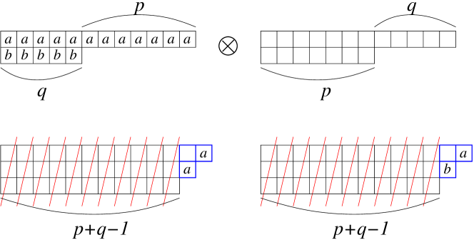
Figure 1: The Young tableaux method of forming the adjoint (octet) representation in the direct product ${\cal R}\otimes\overline{\cal R}$. After making $p+q-1$ singlet combinations, there are two ways of forming an adjoint representation. If $q=0$, the way shown on the right is impossible.

This explicitly shows that the multiplicity $m$ of $\bm{8}$ in ${\cal R}\otimes\overline{\cal R}$ is at most 2.

Similarly, we can show that for $SU(n)$ there are at most $n-1$ ways of forming an adjoint representation from the direct product ${\cal R}\otimes\overline{\cal R}$. This number is just the rank of the group, $\mbox{\rm rank}(G)$, and it is also the number of invariant tensors. The matrix $M^{({\cal R},r)}_{\alpha}$ may be written as a linear combination of $\mbox{\rm rank}(G)$ quantities,

$$T^{({\cal R},s)}_{\alpha}\equiv g_{\alpha\alpha_{1}\alpha_{2}\cdots\alpha_{s}}T^{\cal R}_{\alpha_{1}}T^{\cal R}_{\alpha_{2}}\cdots T^{\cal R}_{\alpha_{s}},\quad(s=1,\cdots,\mbox{\rm rank}(G))$$ (279)

where $g_{\alpha\alpha_{1}\alpha_{2}\cdots\alpha_{s}}$ is a real symmetric invariant tensor of $SU(n)$, and therefore $T^{({\cal R},s)}_{\alpha}$ is Hermitian. For $SU(3)$, there are two symmtric invariant tensors, $\delta_{\alpha\beta}$ and $d_{\alpha\beta\gamma}$. Independence of $T^{({\cal R},s)}_{\alpha}$ may be examined by defining a $\mbox{\rm rank}(G)\times\mbox{\rm rank}(G)$ matrix $C^{st}$,

$$C^{st}id_{\cal R}=T^{({\cal R},s)}_{\alpha}T^{({\cal R},t)}_{\alpha}.$$ (280)

Note that the right hand side commutes with $T^{\cal R}_{\beta}$ for all $\beta$, so that it is proportional to $id_{\cal R}$ by Schur’s lemma. In general, $m=\mbox{\rm rank}(C)\leq\mbox{\rm rank}(G)$. We arrange that the first $m$ $T^{({\cal R},s)}_{\alpha}$’s are independent.

We may now write the matrix $M^{({\cal R},r)}_{\alpha}$ as a linear combination of independent $T^{({\cal R},s)}_{\alpha}$’s,

$$M^{({\cal R},r)}_{\alpha}=\sum_{s=1}^{m}V_{rs}T^{({\cal R},s)}_{\alpha}.$$ (281)

Note that $V_{rs}$ is a regular $m\times m$ matrix, but it is not orthogonal.

The normalization of $M^{({\cal R},r)}_{\alpha}$ is determined by the orthogonality condition of the CG coefficients,

$$\left(\left(M^{({\cal R},r)}_{\alpha}\right)^{\dagger}M^{({\cal R},s)}_{\alpha}\right)_{ij}=\delta_{ij}\delta_{rs}.$$ (282)

By substituting (281) into the above expression, we get

$$\left(VCV^{\dagger}\right)_{rs}=\delta_{rs},$$ (283)

thus,

$$\left(V^{\dagger}V\right)_{rs}=\left(C^{-1}\right)_{rs}.$$ (284)

We can write down (276) in terms of $T^{({\cal R},r)}_{\alpha}$,

$$\int dg\left(D^{\cal R}_{ij}(g)\right)^{*}D^{(8)}_{\alpha\beta}(g)D^{{\cal R}}_{kl}(g) = \frac{1}{\mbox{\rm dim}{\cal R}}\sum_{r=1}^{m}\big{(}M^{({\cal R},r)}_{\alpha}\big{)}_{ik}^{*}\big{(}M^{({\cal R},r)}_{\beta}\big{)}_{jl}$$ (285)

$$= \frac{1}{\mbox{\rm dim}{\cal R}}\sum_{s,t=1}^{m}\left(V^{\dagger}V\right)_{st}\big{(}T^{({\cal R},s)}_{\alpha}\big{)}_{ki}\big{(}T^{({\cal R},t)}_{\beta}\big{)}_{jl}.$$

By substituting (284) into this, we finally get the expression,

$$\int dg\left(D^{\cal R}_{ij}(g)\right)^{*}D^{(8)}_{\alpha\beta}(g)D^{{\cal R}}_{kl}(g)=\frac{1}{\mbox{\rm dim}{\cal R}}\sum_{s,t=1}^{m}\left(C^{-1}\right)_{st}\big{(}T^{({\cal R},s)}_{\alpha}\big{)}_{ki}\big{(}T^{({\cal R},t)}_{\beta}\big{)}_{jl}.$$ (286)

For $SU(n)$, $D^{(8)}(g)$ should be replaced by $D^{Ad}(g)$.

A.3 Formulae for the matrix elements diagonal in representation

Let us now calculate the matrix elements of various operators, which are diagonal in representation, by using the formulae derived in the previous subsection.

For $SU(3)$, there are two symmetric invariant tensors $\delta_{\alpha\beta}$ and $d_{\alpha\beta\gamma}$, we have

$$T^{({\cal R},1)}_{\alpha}\equiv T^{\cal R}_{\alpha},\quad T^{({\cal R},2)}_{\alpha}\equiv d_{\alpha\beta\gamma}T^{\cal R}_{\beta}T^{\cal R}_{\gamma}=D^{\cal R}_{\alpha}.$$ (287)

The matrix $C^{rs}$ may be written as

$$C=\left(\begin{array}[]{cc}C_{2}&C_{3}\\ C_{3}&D_{2}\end{array}\right),$$ (288)

where $C_{2}$ and $C_{3}$ are quadratic and cubic CasimirsBarut:1986dd respectively,

$$C_{2} = \frac{1}{3}\left(p^{2}+q^{2}+pq+3(p+q)\right),$$ (289)

$$C_{3} = \frac{1}{18}(p-q)\left(2p^{2}+2q^{2}+5pq+9(p+q+1)\right),$$ (290)

for representation ${\cal R}=(p,q)$, while $D_{2}\equiv\sum_{\alpha}D^{\cal R}_{\alpha}D^{\cal R}_{\alpha}$ may be written as

$$D_{2}=\left(\frac{1}{3}C_{2}+\frac{1}{4}\right)C_{2}.$$ (291)

By looking at the determinant of $C$,

$$\det C=\frac{1}{12}pq(p+2)(q+2)(p^{2}+q^{2}+2pq+4(p+q)+3),$$ (292)

we see that $T^{\cal R}_{\alpha}$ and $D^{\cal R}_{\alpha}$ are not independent for $p=0$ or $q=0$. Actually,

$$D^{\cal R}_{\alpha}=\frac{C_{3}}{C_{2}}T^{\cal R}_{\alpha}.$$ (293)

In this case, the integral (286) gets simpler,

$$\int dg\left(D^{\cal R}_{ij}(g)\right)^{*}D^{(8)}_{\alpha\beta}(g)D^{{\cal R}}_{kl}(g)=\frac{1}{\mbox{\rm dim}{\cal R}}\frac{1}{C_{2}({\cal R})}\big{(}T^{\cal R}_{\alpha}\big{)}_{ki}\big{(}T^{\cal R}_{\beta}\big{)}_{jl}.$$ (294)

When $\det C\neq 0$, $T^{\cal R}_{\alpha}$ and $D^{\cal R}_{\alpha}$ are independent and the matrix $C$ has the inverse,

$$C^{-1}=\frac{1}{C_{2}^{2}(3+4C_{2})-12C_{3}^{2}}\left(\begin{array}[]{cc}C_{2}(3+4C_{2})&-12C_{3}\\ -12C_{3}&12C_{2}\end{array}\right).$$ (295)

A.3.1 Hamiltonian operators

Here we explicitly use $Y_{R}=1$ and present the results for the various flavor $SU(3)$ operators appeared in the Hamiltonian. They are expressed in terms of flavor $T^{\cal R}_{8}$ and $D^{\cal R}_{8}$, i.e., in the Gell-Mann-OkuboOkubo:1961jc form.

Let us first show explicitly the simplest case.

$$\left\langle\Psi^{{\cal R}}_{F_{2}S_{2}}\left|D^{(8)}_{\alpha\beta}\right|\Psi^{\cal R}_{F_{1}S_{1}}\right\rangle = \mbox{\rm dim}{\cal R}P^{*}(S_{2})P(S_{1})\left(\int dg\left(D^{\cal R}_{F_{2}\tilde{S}_{2}}(g)\right)^{*}D^{(8)}_{\alpha\beta}(g)D^{\cal R}_{F_{1}\tilde{S}_{1}}(g)\right)^{*}$$ (296)

$$= P^{*}(S_{2})P(S_{1})\sum_{s,t=1}^{2}\left(C^{-1}\right)_{st}\big{(}T^{{\cal R},s}_{\alpha}\big{)}_{F_{2}F_{1}}\big{(}T^{{\cal R},t}_{\beta}\big{)}_{\tilde{S}_{1}\tilde{S}_{2}}.$$

Since

$$\left(T^{\cal R}_{8}\right)_{\tilde{S}_{1}\tilde{S}_{2}} = \frac{\sqrt{3}}{2}\delta_{\tilde{S}_{1}\tilde{S}_{2}},$$ (297)

$$\left(D^{\cal R}_{8}\right)_{\tilde{S}_{1}\tilde{S}_{2}} = \frac{\sqrt{3}}{2}\left(\bm{J}^{2}-\frac{1}{3}C_{2}({\cal R})-\frac{1}{4}\right)\delta_{\tilde{S}_{1}\tilde{S}_{2}},$$ (298)

we have

$$\left\langle\Psi^{{\cal R}}_{F_{2}S_{2}}\left|D^{(8)}_{88}\right|\Psi^{\cal R}_{F_{1}S_{1}}\right\rangle = \frac{\sqrt{3}}{2}\bigg{\{}\big{(}T_{8}\big{)}_{F_{2}F_{1}}\left(C^{-1}_{11}+C^{-1}_{12}\left(\bm{J}^{2}-\frac{1}{3}C_{2}-\frac{1}{4}\right)\right)$$ (299)

$${}+\big{(}D_{8}\big{)}_{F_{2}F_{1}}\left(C^{-1}_{21}+C^{-1}_{22}\left(\bm{J}^{2}-\frac{1}{3}C_{2}-\frac{1}{4}\right)\right)\bigg{\}}\delta_{\tilde{S}_{1}\tilde{S}_{2}},$$

where $\bm{J}^{2}$ stands for the spin $SU(2)$ quadratic Casimir. We dropped all the ${\cal R}$ dependence on the right hand side for notational simplicity.

Other matrix elements may be calculated in a similar way. The results are summarized as follows,

$$\left\langle\Psi^{{\cal R}}_{F_{2}S_{2}}\left|{\cal O}_{i}\right|\Psi^{\cal R}_{F_{1}S_{1}}\right\rangle = P^{*}(S_{2})P(S_{1})\bigg{\{}\big{(}T_{8}\big{)}_{F_{2}F_{1}}\left(C^{-1}_{11}O^{(1)}_{i}+C^{-1}_{12}O^{(2)}_{i}\right)_{\tilde{S}_{1}\tilde{S}_{2}}$$ (300)

$${}+\big{(}D_{8}\big{)}_{F_{2}F_{1}}\left(C^{-1}_{21}O^{(1)}_{i}+C^{-1}_{22}O^{(2)}_{i}\right)_{\tilde{S}_{1}\tilde{S}_{2}}\bigg{\}},$$

where

$$O^{(1)}_{x} = \frac{\sqrt{3}}{2}\bm{J}^{2},$$ (301)

$$O^{(2)}_{x} = \frac{\sqrt{3}}{6}\left(3\bm{J}^{2}-C_{2}-\frac{3}{4}\right)\bm{J}^{2},$$ (302)

$$O^{(1)}_{y} = \frac{3}{8}+\frac{1}{2}C_{2}+\frac{2}{3}C_{3}-\frac{3}{2}\bm{J}^{2},$$ (303)

$$O^{(2)}_{y} = -\frac{3}{16}-\frac{1}{4}C_{2}-\frac{1}{3}C_{3}+\frac{1}{2}\bm{J}^{2}+C_{2}\bm{J}^{2}-\left(\bm{J}^{2}\right)^{2},$$ (304)

$$O^{(1)}_{z} = \frac{\sqrt{3}}{2}\left(C_{2}-\bm{J}^{2}-\frac{9}{4}\right),$$ (305)

$$O^{(2)}_{z} = \frac{\sqrt{3}}{6}\left(3\bm{J}^{2}-C_{2}-\frac{3}{4}\right)\left(C_{2}-\bm{J}^{2}-\frac{9}{4}\right),$$ (306)

$$O^{(1)}_{w} = -\frac{3}{8}+\frac{1}{3}C_{3}-\frac{1}{2}\bm{J}^{2},$$ (307)

$$O^{(2)}_{w} = -\frac{3}{32}+\frac{1}{8}C_{2}+\frac{1}{3}\left(C_{2}\right)^{2}+\frac{1}{3}C_{3}-\frac{3}{4}\bm{J}^{2}-\frac{5}{6}C_{2}\bm{J}^{2}+\frac{1}{2}\left(\bm{J}^{2}\right)^{2}.$$ (308)

The usefulness of these formulae rests on the fact that they are easily calculated for arbitrary representation ${\cal R}$.

A.3.2 Decay operators

The matrix elements of the $G_{0}$ operator may be calculated by using Eq. (296),

$$\left\langle\Psi^{{\cal R}}_{F_{2}S_{2}}\left|D^{(8)}_{\alpha i}\right|\Psi^{\cal R}_{F_{1}S_{1}}\right\rangle = P^{*}(S_{2})P(S_{1})\sum_{s,t=1}^{2}\left(C^{-1}\right)_{st}\big{(}T^{{\cal R},s}_{\alpha}\big{)}_{F_{2}F_{1}}\big{(}T^{{\cal R},t}_{i}\big{)}_{\tilde{S}_{1}\tilde{S}_{2}}$$ (309)

$$= P^{*}(S_{2})P(S_{1})\bigg{\{}\big{(}T_{\alpha}\big{)}_{F_{2}F_{1}}\left(C^{-1}_{11}\left(T_{i}\right)_{\tilde{S}_{1}\tilde{S}_{2}}+C^{-1}_{12}\left(D_{i}\right)_{\tilde{S}_{1}\tilde{S}_{2}}\right)$$

$$\qquad{}+\big{(}D_{\alpha}\big{)}_{F_{2}F_{1}}\left(C^{-1}_{21}\left(T_{i}\right)_{\tilde{S}_{1}\tilde{S}_{2}}+C^{-1}_{22}\left(D_{i}\right)_{\tilde{S}_{1}\tilde{S}_{2}}\right)\bigg{\}}.$$

Since $T_{i}$ is the usual spin $SU(2)$ generator, the matrix elements between the states with different spins vanish and only the $D_{i}$ terms contribute. When the both states have the same spin, from the transformation property, $D_{i}$ is proportional to $T_{i}$. By using

$$\sum_{i=1}^{3}T_{i}D_{i}=\frac{1}{3}C_{3}+\frac{1}{2\sqrt{3}}C_{2}T_{8}+\frac{1}{2\sqrt{3}}\bm{J}^{2}T_{8}-\frac{1}{6\sqrt{3}}(T_{8})^{3}+\frac{1}{2\sqrt{3}}T_{8},$$ (310)

we have for the same spin states (with $Y_{R}=1$),

$$\left(D_{i}\right)_{\tilde{S}_{1}\tilde{S}_{2}}=A\left(T_{i}\right)_{\tilde{S}_{1}\tilde{S}_{2}},$$ (311)

with

$$A=\frac{1}{\bm{J}^{2}}\left(\frac{1}{3}C_{3}+\frac{1}{4}C_{2}+\frac{1}{4}\bm{J}^{2}+\frac{3}{16}\right).$$ (312)

The matrix elements, diagonal in representation, of the decay operators which are linear in $F_{\alpha}$ may be calculated in a similar way. For the $G_{2}$ operator, we have

$$\left\langle\Psi^{{\cal R}}_{F_{2}S_{2}}\left|D^{(8)}_{\alpha 8}F_{i}\right|\Psi^{\cal R}_{F_{1}S_{1}}\right\rangle = P^{*}(S_{2})P(S_{1})\sum_{s,t=1}^{2}\left(C^{-1}\right)_{st}\big{(}T^{{\cal R},s}_{\alpha}\big{)}_{F_{2}F_{1}}\big{(}T^{{\cal R},t}_{8}\big{)}_{\tilde{S}^{\prime}_{1}\tilde{S}_{2}}\left(-T^{\cal R}_{i}\right)_{\tilde{S}_{1}\tilde{S}^{\prime}_{1}}.$$

By using Eqs. (297) and (298), this can be rewrite as

$$\left\langle\Psi^{{\cal R}}_{F_{2}S_{2}}\left|D^{(8)}_{\alpha 8}F_{i}\right|\Psi^{\cal R}_{F_{1}S_{1}}\right\rangle=-\frac{\sqrt{3}}{2}P^{*}(S_{2})P(S_{1})\bigg{\{}\big{(}T_{\alpha}\big{)}_{F_{2}F_{1}}\left(C^{-1}_{11}+C^{-1}_{12}\left(\bm{J}^{2}-\frac{1}{3}C_{2}-\frac{1}{4}\right)\right)$$

$$\qquad{}+\big{(}D_{\alpha}\big{)}_{F_{2}F_{1}}\left(C^{-1}_{21}+C^{-1}_{22}\left(\bm{J}^{2}-\frac{1}{3}C_{2}-\frac{1}{4}\right)\right)\bigg{\}}\left(T_{i}\right)_{\tilde{S}_{1}\tilde{S}_{2}}.$$ (314)

Similarly, we can calculate the matrix elements for the $G_{1}$ operator,

$$\left\langle\Psi^{{\cal R}}_{F_{2}S_{2}}\left|\sum_{\beta,\gamma\in{\cal J}}d_{i\beta\gamma}D^{(8)}_{\alpha\beta}F_{\gamma}\right|\Psi^{\cal R}_{F_{1}S_{1}}\right\rangle$$ (315)

$$= -P^{*}(S_{2})P(S_{1})\sum_{s,t=1}^{2}\left(C^{-1}\right)_{st}\big{(}T^{{\cal R},s}_{\alpha}\big{)}_{F_{2}F_{1}}\sum_{\beta,\gamma\in{\cal J}}d_{i\beta\gamma}\big{(}T^{\cal R}_{\gamma}T^{{\cal R},t}_{\beta}\big{)}_{\tilde{S}_{1}\tilde{S}_{2}}.$$

Note that

$$\sum_{\beta,\gamma\in{\cal J}}d_{i\beta\gamma}T_{\beta}T_{\gamma} = D_{i}-\frac{2}{\sqrt{3}}T_{i}T_{8},$$ (316)

$$\sum_{\beta,\gamma\in{\cal J}}d_{i\beta\gamma}T_{\beta}D_{\gamma} = \left(\frac{1}{3}C_{2}+\frac{1}{4}\right)T_{i}-\frac{1}{\sqrt{3}}\left(D_{i}T_{8}+D_{8}T_{i}\right),$$ (317)

we have

$$\left\langle\Psi^{{\cal R}}_{F_{2}S_{2}}\left|\sum_{\beta,\gamma\in{\cal J}}d_{i\beta\gamma}D^{(8)}_{\alpha\beta}F_{\gamma}\right|\Psi^{\cal R}_{F_{1}S_{1}}\right\rangle$$ (318)

$$= -P^{*}(S_{2})P(S_{1})\bigg{\{}\big{(}T_{\alpha}\big{)}_{F_{2}F_{1}}\left(C^{-1}_{11}(D_{i}-T_{i})+C^{-1}_{12}\left(\left(\frac{1}{2}C_{2}-\frac{1}{2}\bm{J}^{2}+\frac{3}{8}\right)T_{i}-\frac{1}{2}D_{i}\right)\right)_{\tilde{S}_{1}\tilde{S}_{2}}$$

$${}+\big{(}D_{\alpha}\big{)}_{F_{2}F_{1}}\left(C^{-1}_{21}(D_{i}-T_{i})+C^{-1}_{22}\left(\left(\frac{1}{2}C_{2}-\frac{1}{2}\bm{J}^{2}+\frac{3}{8}\right)T_{i}-\frac{1}{2}D_{i}\right)\right)_{\tilde{S}_{1}\tilde{S}_{2}}\bigg{\}}.$$

When $\det C=0$, the corresponding formulae become much simpler.

Appendix B Tables of various matrix elements

Those matrix elements of the symmetry breaking operators which are needed to calculated the baryon masses are given in Sec. III.2. In this Appendix, we summarize other matrix elements which are necessary to calculate the mixings to second order.

These matrix elements are calculated with the method explained in the previous section.

To second order, the (mainly) octet states can mix with $\bm{\overline{10}}$, $\bm{27}_{d}$, $\bm{\overline{35}}_{d}$, and $\bm{64}_{d}$. The (mainly) anti-decuplet states can mix with $\bm{\overline{81}}_{d}$ in addition to them. We therefore need $\left\langle\bm{27}_{d}\left|{\cal O}_{i}\right|\bm{27}_{d}\right\rangle$, $\left\langle\bm{\overline{35}}_{d}\left|{\cal O}_{i}\right|\bm{\overline{35}}_{d}\right\rangle$, $\left\langle\bm{\overline{35}}_{d}\left|{\cal O}_{i}\right|\bm{27}_{d}\right\rangle$, $\left\langle\bm{64}_{d}\left|{\cal O}_{i}\right|\bm{27}_{d}\right\rangle$, $\left\langle\bm{64}_{d}\left|{\cal O}_{i}\right|\bm{\overline{35}}_{d}\right\rangle$, and $\left\langle\bm{\overline{81}}_{d}\left|{\cal O}_{i}\right|\bm{\overline{35}}_{d}\right\rangle$.

Table 18: $\left\langle\bm{27}_{d}\left|{\cal O}_{i}\right|\bm{27}_{d}\right\rangle$

$(I,Y)$	$\gamma$	$x$	$y$	$z$	$w$
$(\frac{1}{2},+1)$	$\frac{137}{560}$	$\frac{3}{4}\frac{137}{560}$	$\frac{39\sqrt{3}}{1120}$	$\frac{137}{112}$	$-\frac{2803}{1120\sqrt{3}}$
$(1,0)$	$\frac{13}{280}$	$\frac{3}{4}\frac{13}{280}$	$-\frac{29\sqrt{3}}{560}$	$\frac{13}{56}$	$-\frac{407}{560\sqrt{3}}$
$(\frac{1}{2},-1)$	$\frac{2}{35}$	$\frac{3}{4}\frac{2}{35}$	$-\frac{13\sqrt{3}}{35}$	$\frac{2}{7}$	$-\frac{311}{140\sqrt{3}}$
$(0,0)$	$\frac{13}{70}$	$\frac{3}{4}\frac{13}{70}$	$-\frac{29\sqrt{3}}{140}$	$\frac{13}{14}$	$-\frac{407}{140\sqrt{3}}$
$(\frac{3}{2},-1)$	$-\frac{17}{112}$	$-\frac{3}{4}\frac{17}{112}$	$-\frac{31\sqrt{3}}{224}$	$-\frac{85}{112}$	$\frac{235}{224\sqrt{3}}$

Table 19: $\left\langle\bm{\overline{35}}_{d}\left|{\cal O}_{i}\right|\bm{\overline{35}}_{d}\right\rangle$

$(I,Y)$	$\gamma$	$x$	$y$	$z$	$w$
$(0,+2)$	$\frac{1}{4}$	$\frac{3}{4}\frac{1}{4}$	$-\frac{5\sqrt{3}}{8}$	$\frac{9}{4}$	$-\frac{13\sqrt{3}}{8}$
$(\frac{1}{2},+1)$	$\frac{3}{16}$	$\frac{3}{4}\frac{3}{16}$	$-\frac{11\sqrt{3}}{32}$	$\frac{27}{16}$	$-\frac{43\sqrt{3}}{32}$
$(1,0)$	$\frac{1}{8}$	$\frac{3}{4}\frac{1}{8}$	$-\frac{\sqrt{3}}{16}$	$\frac{9}{8}$	$-\frac{17\sqrt{3}}{16}$
$(\frac{3}{2},-1)$	$\frac{1}{16}$	$\frac{3}{4}\frac{1}{16}$	$\frac{7\sqrt{3}}{32}$	$\frac{9}{16}$	$-\frac{25\sqrt{3}}{32}$

Table 20: $\left\langle\bm{\overline{35}}_{d}\left|{\cal O}_{i}\right|\bm{27}_{d}\right\rangle$

$(I,Y)$	$\gamma$	$x$	$y$	$z$	$w$
$(\frac{1}{2},+1)$	$\frac{\sqrt{15}}{16\sqrt{7}}$	$\frac{3}{4}\frac{\sqrt{15}}{16\sqrt{7}}$	$\frac{17\sqrt{5}}{32\sqrt{7}}$	$\frac{\sqrt{105}}{16}$	$-\frac{11\sqrt{5}}{32\sqrt{7}}$
$(1,0)$	$\frac{\sqrt{5}}{8\sqrt{7}}$	$\frac{3}{4}\frac{\sqrt{5}}{8\sqrt{7}}$	$\frac{17\sqrt{5}}{16\sqrt{21}}$	$\frac{\sqrt{35}}{8}$	$-\frac{11\sqrt{5}}{16\sqrt{21}}$
$(\frac{3}{2},-1)$	$\frac{\sqrt{15}}{16\sqrt{7}}$	$\frac{3}{4}\frac{\sqrt{15}}{16\sqrt{7}}$	$\frac{17\sqrt{5}}{32\sqrt{7}}$	$\frac{\sqrt{105}}{16}$	$-\frac{11\sqrt{5}}{32\sqrt{7}}$

Table 21: $\left\langle\bm{64}_{d}\left|{\cal O}_{i}\right|\bm{27}_{d}\right\rangle$

$(I,Y)$	$\gamma$	$x$	$y$	$z$	$w$
$(\frac{1}{2},+1)$	$\frac{5\sqrt{3}}{28}$	$\frac{3}{4}\frac{5\sqrt{3}}{28}$	$-\frac{5}{14}$	$\frac{85\sqrt{3}}{56}$	$\frac{5}{56}$
$(1,0)$	$\frac{5\sqrt{5}}{28\sqrt{2}}$	$\frac{3}{4}\frac{5\sqrt{5}}{28\sqrt{2}}$	$-\frac{5\sqrt{5}}{14\sqrt{6}}$	$\frac{85\sqrt{5}}{56\sqrt{2}}$	$\frac{5\sqrt{5}}{56\sqrt{6}}$
$(\frac{3}{2},-1)$	$\frac{5\sqrt{3}}{28\sqrt{2}}$	$\frac{3}{4}\frac{5\sqrt{3}}{28\sqrt{2}}$	$-\frac{5}{14\sqrt{2}}$	$\frac{85\sqrt{3}}{56\sqrt{2}}$	$\frac{5}{56\sqrt{2}}$
$(\frac{1}{2},-1)$	$\frac{5\sqrt{3}}{28}$	$\frac{3}{4}\frac{5\sqrt{3}}{28}$	$-\frac{5}{14}$	$\frac{85\sqrt{3}}{56}$	$\frac{5}{56}$
$(0,0)$	$\frac{3\sqrt{5}}{14\sqrt{2}}$	$\frac{3}{4}\frac{3\sqrt{5}}{14\sqrt{2}}$	$-\frac{\sqrt{15}}{7\sqrt{2}}$	$\frac{51\sqrt{5}}{28\sqrt{2}}$	$\frac{\sqrt{15}}{28\sqrt{2}}$

Table 22: $\left\langle\bm{64}_{d}\left|{\cal O}_{i}\right|\bm{\overline{35}}_{d}\right\rangle$

$(I,Y)$	$\gamma$	$x$	$y$	$z$	$w$
$(\frac{1}{2},+1)$	$\frac{1}{4\sqrt{35}}$	$\frac{3}{4}\frac{1}{4\sqrt{35}}$	$\sqrt{\frac{3}{35}}$	$\frac{3\sqrt{7}}{8\sqrt{5}}$	$-\frac{13\sqrt{3}}{8\sqrt{35}}$
$(1,0)$	$\frac{1}{4\sqrt{14}}$	$\frac{3}{4}\frac{1}{4\sqrt{14}}$	$\sqrt{\frac{3}{14}}$	$\frac{3\sqrt{7}}{8\sqrt{2}}$	$-\frac{13\sqrt{3}}{8\sqrt{14}}$
$(\frac{3}{2},-1)$	$\frac{3}{4\sqrt{70}}$	$\frac{3}{4}\frac{3}{4\sqrt{70}}$	$\frac{3\sqrt{3}}{\sqrt{70}}$	$\frac{9\sqrt{7}}{8\sqrt{10}}$	$-\frac{39\sqrt{3}}{8\sqrt{70}}$

Table 23: $\left\langle\bm{\overline{81}}_{d}\left|{\cal O}_{i}\right|\bm{\overline{35}}_{d}\right\rangle$

$(I,Y)$	$\gamma$	$x$	$y$	$z$	$w$
$(0,+2)$	$\frac{\sqrt{3}}{2\sqrt{7}}$	$\frac{3}{4}\frac{\sqrt{3}}{2\sqrt{7}}$	$-\frac{1}{4\sqrt{7}}$	$\frac{13\sqrt{3}}{2\sqrt{7}}$	$\frac{1}{4\sqrt{7}}$
$(\frac{1}{2},+1)$	$\frac{2}{\sqrt{35}}$	$\frac{3}{4}\frac{2}{\sqrt{35}}$	$-\frac{1}{\sqrt{105}}$	$\frac{26}{\sqrt{35}}$	$\frac{1}{\sqrt{105}}$
$(1,0)$	$\frac{\sqrt{3}}{2\sqrt{7}}$	$\frac{3}{4}\frac{\sqrt{3}}{2\sqrt{7}}$	$-\frac{1}{4\sqrt{7}}$	$\frac{13\sqrt{3}}{2\sqrt{7}}$	$\frac{1}{4\sqrt{7}}$
$(\frac{3}{2},-1)$	$\sqrt{\frac{3}{35}}$	$\frac{3}{4}\sqrt{\frac{3}{35}}$	$-\frac{1}{2\sqrt{35}}$	$\frac{13\sqrt{3}}{\sqrt{35}}$	$\frac{1}{2\sqrt{35}}$

The (mainly) decuplet states can mix with $\bm{27}_{q}$, $\bm{35}$, $\bm{\overline{35}}_{q}$, $\bm{64}_{q}$, and $\bm{81}$. Thus we need $\left\langle\bm{27}_{q}\left|{\cal O}_{i}\right|\bm{27}_{q}\right\rangle$, $\left\langle\bm{35}\left|{\cal O}_{i}\right|\bm{35}\right\rangle$, $\left\langle\bm{35}\left|{\cal O}_{i}\right|\bm{27}_{q}\right\rangle$, $\left\langle\bm{\overline{35}}_{q}\left|{\cal O}_{i}\right|\bm{27}_{q}\right\rangle$, $\left\langle\bm{64}_{q}\left|{\cal O}_{i}\right|\bm{27}_{q}\right\rangle$, $\left\langle\bm{64}_{q}\left|{\cal O}_{i}\right|\bm{35}\right\rangle$, and $\left\langle\bm{81}\left|{\cal O}_{i}\right|\bm{35}\right\rangle$.

Table 24: $\left\langle\bm{27}_{q}\left|{\cal O}_{i}\right|\bm{27}_{q}\right\rangle$

$(I,Y)$	$\gamma$	$x$	$y$	$z$	$w$
$(\frac{3}{2},+1)$	$\frac{13}{112}$	$\frac{15}{4}\frac{13}{112}$	$\frac{45\sqrt{3}}{224}$	$\frac{13}{56}$	$-\frac{11}{32\sqrt{3}}$
$(1,0)$	$-\frac{1}{56}$	$-\frac{15}{4}\frac{1}{56}$	$-\frac{25\sqrt{3}}{112}$	$-\frac{1}{28}$	$-\frac{1}{16\sqrt{3}}$
$(\frac{1}{2},-1)$	$-\frac{17}{112}$	$-\frac{15}{4}\frac{17}{112}$	$-\frac{145\sqrt{3}}{224}$	$-\frac{17}{56}$	$\frac{7}{32\sqrt{3}}$

Table 25: $\left\langle\bm{35}\left|{\cal O}_{i}\right|\bm{35}\right\rangle$

$(I,Y)$	$\gamma$	$x$	$y$	$z$	$w$
$(\frac{3}{2},+1)$	$\frac{3}{16}$	$\frac{15}{4}\frac{3}{16}$	$\frac{11\sqrt{3}}{32}$	$\frac{9}{8}$	$-\frac{17\sqrt{3}}{32}$
$(1,0)$	$\frac{1}{8}$	$\frac{15}{4}\frac{1}{8}$	$-\frac{3\sqrt{3}}{16}$	$\frac{3}{4}$	$-\frac{11\sqrt{3}}{16}$
$(\frac{1}{2},-1)$	$\frac{1}{16}$	$\frac{15}{4}\frac{1}{16}$	$-\frac{23\sqrt{3}}{32}$	$\frac{3}{8}$	$-\frac{27\sqrt{3}}{32}$
$(0,-2)$	$0$	$0$	$-\frac{5\sqrt{3}}{4}$	$0$	$-\sqrt{3}$

Table 26: $\left\langle\bm{35}\left|{\cal O}_{i}\right|\bm{27}_{q}\right\rangle$

$(I,Y)$	$\gamma$	$x$	$y$	$z$	$w$
$(\frac{3}{2},+1)$	$\frac{\sqrt{15}}{16\sqrt{7}}$	$\frac{15}{4}\frac{\sqrt{15}}{16\sqrt{7}}$	$-\frac{\sqrt{5}}{32\sqrt{7}}$	$\frac{\sqrt{15}}{4\sqrt{7}}$	$-\frac{17\sqrt{5}}{32\sqrt{7}}$
$(1,0)$	$\frac{\sqrt{5}}{8\sqrt{7}}$	$\frac{15}{4}\frac{\sqrt{5}}{8\sqrt{7}}$	$-\frac{\sqrt{5}}{16\sqrt{21}}$	$\frac{\sqrt{5}}{2\sqrt{7}}$	$-\frac{17\sqrt{5}}{16\sqrt{21}}$
$(\frac{1}{2},-1)$	$\frac{\sqrt{15}}{16\sqrt{7}}$	$\frac{15}{4}\frac{\sqrt{15}}{16\sqrt{7}}$	$-\frac{\sqrt{5}}{32\sqrt{7}}$	$\frac{\sqrt{15}}{4\sqrt{7}}$	$-\frac{17\sqrt{5}}{32\sqrt{7}}$

Table 27: $\left\langle\bm{\overline{35}}_{q}\left|{\cal O}_{i}\right|\bm{27}_{q}\right\rangle$

$(I,Y)$	$\gamma$	$x$	$y$	$z$	$w$
$(\frac{3}{2},+1)$	$\sqrt{\frac{3}{35}}$	$\frac{15}{4}\sqrt{\frac{3}{35}}$	$\frac{\sqrt{5}}{2\sqrt{7}}$	$\frac{4\sqrt{3}}{\sqrt{35}}$	$-\frac{\sqrt{5}}{2\sqrt{7}}$
$(1,0)$	$\frac{1}{2\sqrt{7}}$	$\frac{15}{4}\frac{1}{2\sqrt{7}}$	$\frac{5}{4\sqrt{21}}$	$\frac{2}{\sqrt{7}}$	$-\frac{5}{4\sqrt{21}}$

Table 28: $\left\langle\bm{64}_{q}\left|{\cal O}_{i}\right|\bm{27}_{q}\right\rangle$

$(I,Y)$	$\gamma$	$x$	$y$	$z$	$w$
$(\frac{3}{2},+1)$	$\frac{5\sqrt{3}}{56}$	$\frac{15}{4}\frac{5\sqrt{3}}{56}$	$-\frac{5}{7}$	$\frac{55\sqrt{3}}{112}$	$\frac{5}{16}$
$(1,0)$	$\frac{5\sqrt{5}}{56}$	$\frac{15}{4}\frac{5\sqrt{5}}{56}$	$-\frac{5\sqrt{5}}{7\sqrt{3}}$	$\frac{55\sqrt{5}}{112}$	$\frac{5\sqrt{5}}{16\sqrt{3}}$
$(\frac{1}{2},-1)$	$\frac{5\sqrt{3}}{28\sqrt{2}}$	$\frac{15}{4}\frac{5\sqrt{3}}{28\sqrt{2}}$	$-\frac{5\sqrt{2}}{\sqrt{7}}$	$\frac{55\sqrt{3}}{56\sqrt{2}}$	$\frac{5}{8\sqrt{2}}$
$(0,0)$	$\frac{3\sqrt{5}}{28}$	$\frac{15}{4}\frac{3\sqrt{5}}{28}$	$-\frac{2\sqrt{15}}{7}$	$\frac{33\sqrt{5}}{56}$	$\frac{\sqrt{15}}{8}$

Table 29: $\left\langle\bm{64}_{q}\left|{\cal O}_{i}\right|\bm{35}\right\rangle$

$(I,Y)$	$\gamma$	$x$	$y$	$z$	$w$
$(\frac{3}{2},+1)$	$\frac{9}{8\sqrt{35}}$	$\frac{15}{4}\frac{9}{8\sqrt{35}}$	$\frac{3\sqrt{15}}{4\sqrt{7}}$	$\frac{27\sqrt{5}}{16\sqrt{7}}$	$-\frac{51\sqrt{3}}{16\sqrt{35}}$
$(1,0)$	$\frac{3}{8\sqrt{7}}$	$\frac{15}{4}\frac{3}{8\sqrt{7}}$	$\frac{5\sqrt{3}}{4\sqrt{7}}$	$\frac{45}{16\sqrt{7}}$	$-\frac{17\sqrt{3}}{16\sqrt{7}}$
$(\frac{1}{2},-1)$	$\frac{3}{4\sqrt{70}}$	$\frac{15}{4}\frac{3}{4\sqrt{70}}$	$\frac{\sqrt{15}}{2\sqrt{14}}$	$\frac{9\sqrt{5}}{8\sqrt{14}}$	$-\frac{17\sqrt{3}}{8\sqrt{70}}$

Table 30: $\left\langle\bm{81}\left|{\cal O}_{i}\right|\bm{35}\right\rangle$

$(I,Y)$	$\gamma$	$x$	$y$	$z$	$w$
$(\frac{3}{2},+1)$	$\frac{3}{2\sqrt{35}}$	$\frac{15}{4}\frac{3}{2\sqrt{35}}$	$-\frac{3\sqrt{15}}{4\sqrt{7}}$	$\frac{3\sqrt{5}}{\sqrt{7}}$	$\frac{3\sqrt{3}}{4\sqrt{35}}$
$(1,0)$	$\frac{3}{4\sqrt{7}}$	$\frac{15}{4}\frac{3}{4\sqrt{7}}$	$-\frac{15\sqrt{3}}{8\sqrt{7}}$	$\frac{15}{2\sqrt{7}}$	$\frac{3\sqrt{3}}{8\sqrt{7}}$
$(\frac{1}{2},-1)$	$\sqrt{\frac{3}{35}}$	$\frac{15}{4}\sqrt{\frac{3}{35}}$	$-\frac{3\sqrt{5}}{2\sqrt{7}}$	$\frac{2\sqrt{15}}{\sqrt{7}}$	$\frac{3}{2\sqrt{35}}$
$(0,-2)$	$\frac{3}{4\sqrt{7}}$	$\frac{15}{4}\frac{3}{4\sqrt{7}}$	$-\frac{15\sqrt{3}}{8\sqrt{7}}$	$\frac{15}{2\sqrt{7}}$	$\frac{3\sqrt{3}}{8\sqrt{7}}$

Because these matrix elements listed above only contribute to the second order calculations, those of ${\cal O}_{v_{1}}$ and ${\cal O}_{v_{2}}$ are not necessary, because these operators themselves are of second order. There are, however, extra matrix elements that we need to calculate; $\left\langle\bm{\overline{35}}_{d}\left|{\cal O}_{v}\right|\bm{8}\right\rangle$, $\left\langle\bm{64}_{d}\left|{\cal O}_{v}\right|\bm{8}\right\rangle$, $\left\langle\bm{64}_{d}\left|{\cal O}_{v}\right|\bm{\overline{10}}\right\rangle$, $\left\langle\bm{\overline{81}}_{d}\left|{\cal O}_{v}\right|\bm{\overline{10}}\right\rangle$, $\left\langle\bm{\overline{35}}_{q}\left|{\cal O}_{v}\right|\bm{10}\right\rangle$, $\left\langle\bm{64}_{q}\left|{\cal O}_{v}\right|\bm{10}\right\rangle$, and $\left\langle\bm{81}\left|{\cal O}_{v}\right|\bm{10}\right\rangle$.

Table 31: $\left\langle\bm{\overline{35}}_{d}\left|{\cal O}_{v}\right|\bm{8}\right\rangle$ & $\left\langle\bm{64}_{d}\left|{\cal O}_{v}\right|\bm{8}\right\rangle$

	$\left\langle\bm{\overline{35}}_{d}\left|{\cal O}_{v}\right|\bm{8}\right\rangle$		$\left\langle\bm{64}_{d}\left|{\cal O}_{v}\right|\bm{8}\right\rangle$
(I,Y)	$v_{1}$	$v_{2}$	$v_{1}$	$v_{2}$
$(\frac{1}{2},1)$	$\frac{3}{4\sqrt{70}}$	$\frac{1}{4\sqrt{70}}$	$\frac{3}{28\sqrt{2}}$	$\frac{1}{28\sqrt{2}}$
$(1,0)$	$\frac{1}{2\sqrt{35}}$	$\frac{1}{6\sqrt{35}}$	$\frac{\sqrt{5}}{28\sqrt{2}}$	$\frac{\sqrt{5}}{84\sqrt{2}}$
$(\frac{1}{2},-1)$	0	0	$\frac{3}{28\sqrt{2}}$	$\frac{1}{28\sqrt{2}}$
$(0,0)$	0	0	$\frac{9}{28\sqrt{10}}$	$\frac{3}{28\sqrt{10}}$

Table 32: $\left\langle\bm{64}_{d}\left|{\cal O}_{v}\right|\bm{\overline{10}}\right\rangle$ & $\left\langle\bm{\overline{81}}_{d}\left|{\cal O}_{v}\right|\bm{\overline{10}}\right\rangle$

	$\left\langle\bm{64}_{d}\left|{\cal O}_{v}\right|\bm{\overline{10}}\right\rangle$		$\left\langle\bm{\overline{81}}_{d}\left|{\cal O}_{v}\right|\bm{\overline{10}}\right\rangle$
(I,Y)	$v_{1}$	$v_{2}$	$v_{1}$	$v_{2}$
$(0,2)$	0	0	$\frac{3\sqrt{3}}{56}$	$\frac{\sqrt{3}}{56}$
$(\frac{1}{2},1)$	$\frac{3}{28\sqrt{10}}$	$\frac{1}{28\sqrt{10}}$	$\frac{9}{28\sqrt{10}}$	$\frac{3}{28\sqrt{10}}$
$(1,0)$	$\frac{1}{14\sqrt{2}}$	$\frac{1}{42\sqrt{2}}$	$\frac{3\sqrt{3}}{56}$	$\frac{\sqrt{3}}{56}$
$(\frac{3}{2},-1)$	$\frac{3}{56}$	$\frac{1}{56}$	$\frac{3\sqrt{3}}{56\sqrt{2}}$	$\frac{\sqrt{3}}{56\sqrt{2}}$

Table 33: $\left\langle\bm{\overline{35}}_{q}\left|{\cal O}_{v}\right|\bm{10}\right\rangle$, $\left\langle\bm{64}_{q}\left|{\cal O}_{v}\right|\bm{10}\right\rangle$ & $\left\langle\bm{81}\left|{\cal O}_{v}\right|\bm{10}\right\rangle$

	$\left\langle\bm{\overline{35}}_{q}\left|{\cal O}_{v}\right|\bm{10}\right\rangle$		$\left\langle\bm{64}_{q}\left|{\cal O}_{v}\right|\bm{10}\right\rangle$		$\left\langle\bm{81}\left|{\cal O}_{v}\right|\bm{10}\right\rangle$
(I,Y)	$v_{1}$	$v_{2}$	$v_{1}$	$v_{2}$	$v_{1}$	$v_{2}$
$(\frac{3}{2},1)$	$\frac{\sqrt{5}}{6\sqrt{2}}$	$\frac{\sqrt{5}}{18\sqrt{2}}$	$\frac{3\sqrt{5}}{56\sqrt{2}}$	$\frac{\sqrt{5}}{56\sqrt{2}}$	$\frac{3\sqrt{5}}{112\sqrt{2}}$	$\frac{\sqrt{5}}{112\sqrt{2}}$
$(1,0)$	$\frac{\sqrt{5}}{6\sqrt{2}}$	$\frac{\sqrt{5}}{18\sqrt{2}}$	$\frac{\sqrt{5}}{28}$	$\frac{\sqrt{5}}{84}$	$\frac{3\sqrt{5}}{112}$	$\frac{\sqrt{5}}{112}$
$(\frac{1}{2},-1)$	0	0	$\frac{3}{56}$	$\frac{1}{56}$	$\frac{3\sqrt{3}}{56\sqrt{2}}$	$\frac{\sqrt{3}}{56\sqrt{2}}$
$(0,-2)$	0	0	0	0	$\frac{3\sqrt{5}}{112}$	$\frac{\sqrt{5}}{112}$

Appendix C “Traditional” Approach to the Skyrme Model

In this section, we consider the “traditional” approach to the action (13). Namely, we calculate the profile function $F(r)$ of the soliton, then all of the Skyrme model parameters are determined by the $\chi$PT parameters and the integrations involving the profile function.

It has been known that, in the conventional Skyrme model where ${\cal O}_{\gamma}$ is the only symmetry breaking interaction, the physical values of the $\chi$PT parameters do not reproduce the baryon mass spectrum. In particular, the best fit value of the pion decay constant $F_{\pi}$ is typically less than one third of the physical value (e.g., $46$ MeVPraszalowicz:1985bt for the physical value $184.8$ MeV), while the Kaon mass (if it is treated as a parameter) becomes quite large (around $800$ MeV).

From the effective theory point of view, this discrepancy can be understood easily. There are an infinite number of operators in the $\chi$PT action and they contribute to the Skyrme model parameters. The conventional Skyrme model ignores all of such contributions from the higher order terms. Furthermore, we do not know those coupling constants at all. In this paper, we therefore give up to “calculate” the Skyrme model parameters from the $\chi$PT parameters, and fit them directly to the experimental values.

An important question is whether the best fit values of the $\chi$PT parameters “improve” as we systematically take the higher order contributions into account. In this Appendix, we address this question. Starting with the action (13), we calculate the profile function and the Skyrme model parameters. By fitting them to the experimental values of the baryon masses, we obtain the best fit values of the $\chi$PT parameters.

C.1 Profile function $F(r)$

First of all, it is useful to define the subtracted action $S_{sub}[U]$ as

$$S_{sub}[U]\equiv S[U]-\frac{F_{0}^{2}B_{0}}{8}\int d^{4}x\mbox{\rm Tr}\left({\cal M}^{\dagger}+{\cal M}\right)-L_{8}B_{0}^{2}\int d^{4}x\mbox{\rm Tr}\left({\cal M}^{\dagger}{\cal M}^{\dagger}+{\cal M}{\cal M}\right),$$ (319)

so that $S_{sub}[U=1]=0$.

The profile function $F(r)$ minimizes $M[F]$ defined by

$$S_{sub}[U_{c}]=-M[F]\int dt,$$ (320)

subject to the boundary conditions,

$$F(0)=\pi,\quad F(\infty)=0.$$ (321)

The minimum is called $M_{cl}$,

$$M_{cl}=\min_{F(r)}M[F].$$ (322)

The profile function satisfies the Euler-Lagrange equation,

$$\frac{d}{d{r}}\frac{\partial M}{\partial(dF/dr)}-\frac{\partial M}{\partial F}=0.$$ (323)

By substituting the solution $F(r)$, we obtain $M_{cl}$,

$$M_{cl} = \frac{4\pi F_{0}}{e}\int_{0}^{\infty}\tilde{r}^{2}d\tilde{r}\bigg{[}\frac{1}{8}\left\{\left(F^{\prime}\right)^{2}+\frac{2\sin^{2}F}{\tilde{r}^{2}}\right\}+\frac{\sin^{2}F}{2\tilde{r}^{2}}\left\{2\left(F^{\prime}\right)^{2}+\frac{\sin^{2}F}{\tilde{r}^{2}}\right\}$$ (324)

$${}+\frac{mB_{0}}{2F_{0}^{2}e^{2}}\left(1-\cos F\right)+\frac{4mB_{0}L_{5}}{F_{0}^{2}}\cos F\left\{\left(F^{\prime}\right)^{2}+\frac{2\sin^{2}F}{\tilde{r}^{2}}\right\}$$

$${}+\frac{8m^{2}B_{0}^{2}L_{8}}{F_{0}^{4}e^{2}}\sin^{2}F\bigg{]},$$

where we have introduced $\tilde{r}=F_{0}er$ and $F^{\prime}=dF/d\tilde{r}$. Note that there are higher order contributions and they affect the behavior of the profile function, and hence the values of the other parameters. The existence of the higher order interactions affects the values of the parameters in two ways; through the behavior of the profile function and the new terms from the higher order interactions.

For a large value of $r$, $F(r)$ and its derivative behave like $F\sim 0$, $F^{\prime}\sim 0$, and thus $\sin F\sim F$, $\cos F\sim 1$, we have

$$\frac{\partial M}{\partial F^{\prime}} \sim \frac{4\pi F_{0}}{e}\left(\frac{1}{4}+\frac{8mB_{0}L_{5}}{F_{0}^{2}}\right)\tilde{r}^{2}F^{\prime},$$ (325)

$$\frac{\partial M}{\partial F} \sim \frac{4\pi F_{0}}{e}\left(\frac{mB_{0}}{2F_{0}^{2}e^{2}}+\frac{16m^{2}B_{0}^{2}L_{8}}{F_{0}^{4}e^{2}}\right)\tilde{r}^{2}F.$$ (326)

By solving the Euler-Lagrange equation, the asymptotic behavior,

$$F(\tilde{r})\sim\frac{e^{-\mu\tilde{r}}}{\tilde{r}},$$ (327)

is obtained, where $\mu$ is given by

$$\mu = \frac{\sqrt{2mB_{0}}}{F_{0}e}\sqrt{\frac{1+\frac{32mB_{0}L8}{F_{0}^{2}}}{1+\frac{32mB_{0}L_{5}}{F_{0}^{2}}}}$$ (328)

$$\approx \frac{\sqrt{2mB_{0}}}{F_{0}e}\left(1+\frac{16mB_{0}}{F_{0}^{2}}(L_{8}-L_{5})\right).$$

Note that $\mu$ is close to the pion mass but not exactly the same.

C.2 Inertia tensor $I_{\alpha\beta}(A)$

After substituting $U=AU_{c}A^{\dagger}$ into $S_{sub}[U]$, the inertia tensor can be easily read off as the coefficients of the terms quadratic in the “angular velocity” $\omega^{\alpha}$,

$$I_{\alpha\beta}(A) = -\frac{F_{0}^{2}}{16}\int d^{3}x\frac{1}{2}\mbox{\rm Tr}\left[\lambda_{\alpha}U_{c}^{\dagger}\lambda_{\beta}U_{c}+\lambda_{\beta}U_{c}^{\dagger}\lambda_{\alpha}U_{c}-\{\lambda_{\alpha},\lambda_{\beta}\}\right]$$ (329)

$$+{}\frac{1}{128e^{2}}\int d^{3}x\mbox{\rm Tr}\left([U_{c}^{\dagger}\lambda_{\alpha}U_{c}-\lambda_{\alpha},U_{c}^{\dagger}\partial_{i}U_{c}][U_{c}^{\dagger}\lambda_{\beta}U_{c}-\lambda_{\beta},U_{c}^{\dagger}\partial_{i}U_{c}]\right)$$

$${}-\frac{2L_{5}B_{0}}{3}\frac{2m+m_{s}}{3}\int d^{3}x\left(1+2\cos F\right)\frac{1}{2}\mbox{\rm Tr}\left[\lambda_{\alpha}U_{c}^{\dagger}\lambda_{\beta}U_{c}+\lambda_{\beta}U_{c}^{\dagger}\lambda_{\alpha}U_{c}-\{\lambda_{\alpha},\lambda_{\beta}\}\right]$$

$${}+\frac{L_{5}B_{0}}{\sqrt{3}}\frac{2m+m_{s}}{3}\int d^{3}x\left(1-\cos F\right)\frac{1}{2}\mbox{\rm Tr}\bigg{[}\lambda_{8}\big{(}\lambda_{\alpha}U_{c}^{\dagger}\lambda_{\beta}U_{c}+\lambda_{\beta}U_{c}^{\dagger}\lambda_{\alpha}U_{c}$$

$${}\qquad\qquad\qquad\qquad\qquad+U_{c}^{\dagger}\lambda_{\alpha}U_{c}\lambda_{\beta}+U_{c}^{\dagger}\lambda_{\beta}U_{c}\lambda_{\alpha}-2\{\lambda_{\alpha},\lambda_{\beta}\}\big{)}\bigg{]}$$

$${}-\frac{L_{5}B_{0}}{2}\frac{m_{s}-m}{\sqrt{3}}\int d^{3}x\frac{1}{2}\mbox{\rm Tr}\big{[}(A^{\dagger}\lambda_{8}A)\big{(}\left[\lambda_{\alpha},U_{c}\right]U_{c}^{\dagger}\left[\lambda_{\beta},U_{c}\right]+\left[\lambda_{\beta},U_{c}\right]U_{c}^{\dagger}\left[\lambda_{\alpha},U_{c}\right]$$

$${}\qquad\qquad\qquad\qquad+\left[\lambda_{\alpha},U_{c}^{\dagger}\right]U_{c}\left[\lambda_{\beta},U_{c}^{\dagger}\right]+\left[\lambda_{\beta},U_{c}^{\dagger}\right]U_{c}\left[\lambda_{\alpha},U_{c}^{\dagger}\right]\big{)}\big{]}$$

$$= I_{\alpha\beta}^{0}+I^{\prime}_{\alpha\beta}(A).$$

The $A$-independent part $I_{\alpha\beta}^{0}$ may be written as Eq. (28) with

$$I_{1} = \frac{2\pi}{3e^{3}F_{0}}\int_{0}^{\infty}\tilde{r}^{2}d\tilde{r}\sin^{2}F\left[1+4\left\{\left(F^{\prime}\right)^{2}+\frac{\sin^{2}F}{\tilde{r}^{2}}\right\}+\frac{32\overline{m}B_{0}}{F_{0}^{2}}L_{5}\cos F\right],$$ (330)

$$I_{2} = \frac{\pi}{2e^{3}F_{0}}\int_{0}^{\infty}\tilde{r}^{2}d\tilde{r}(1-\cos F)\left[1+\left(F^{\prime}\right)^{2}+\frac{2\sin^{2}F}{\tilde{r}^{2}}+\frac{8\overline{m}B_{0}}{F_{0}^{2}}L_{5}\left(1+\cos F\right)\right],$$ (331)

where

$$\overline{m}=\frac{2m+m_{s}}{3}$$ (332)

has been introduced.

The $A$-dependent part $I^{\prime}_{\alpha\beta}(A)$ has the complicated structure as Eq. (35). The parameters are now expressed as

$$\overline{x} = -\frac{64\pi L_{5}B_{0}}{9e^{3}F_{0}^{3}}\delta m\int_{0}^{\infty}\tilde{r}^{2}d\tilde{r}\cos F\sin^{2}F,$$ (333)

$$\overline{y} = -\frac{32\pi L_{5}B_{0}}{3\sqrt{3}e^{3}F_{0}^{3}}\delta m\int_{0}^{\infty}\tilde{r}^{2}d\tilde{r}\sin^{2}F,$$ (334)

$$\overline{z} = \frac{32\pi L_{5}B_{0}}{9e^{3}F_{0}^{3}}\delta m\int_{0}^{\infty}\tilde{r}^{2}d\tilde{r}(1-\cos F)(2-\cos F),$$ (335)

$$\overline{w} = \frac{16\pi L_{5}B_{0}}{3\sqrt{3}e^{3}F_{0}^{3}}\delta m\int_{0}^{\infty}\tilde{r}^{2}d\tilde{r}(1-\cos F)(2-\cos F).$$ (336)

C.3 Potential

The “angular velocity” independent part (except for $M_{cl}$) of the Lagrangian is the potential part Eq. (37), $-V(A)$. The parameter $\gamma$ in the first-order term (38) is given by

$$\gamma=\gamma_{0}+\delta_{1}\gamma+\delta_{2}\gamma,$$ (337)

with

$$\gamma_{0} = \delta m\frac{4\pi B_{0}}{3e^{3}F_{0}}\int_{0}^{\infty}\tilde{r}^{2}d\tilde{r}(1-\cos F),$$ (338)

$$\delta_{1}\gamma = \delta m\frac{32\pi B_{0}L_{5}}{3eF_{0}}\int_{0}^{\infty}\tilde{r}^{2}d\tilde{r}\cos F\left(\left(F^{\prime}\right)^{2}+\frac{2\sin^{2}F}{\tilde{r}^{2}}\right),$$ (339)

$$\delta_{2}\gamma = \delta m\frac{64\pi\overline{m}B_{0}^{2}L_{8}}{3e^{3}F_{0}^{3}}\int_{0}^{\infty}\tilde{r}^{2}d\tilde{r}\left(1-\cos 2F\right).$$ (340)

The parameter $v$ in the second-order term (39) is given by

$$v = \left(\delta m\right)^{2}\frac{16\pi B_{0}^{2}L_{8}}{9e^{3}F_{0}^{3}}\int_{0}^{\infty}\tilde{r}^{2}d\tilde{r}\left(1-\cos F\right)\left(1-2\cos F\right).$$ (341)

C.4 Numerical calculations

Starting with the $\chi$PT parameters $F_{0}$, $B_{0}$, $e$, $L_{5}$, $L_{8}$, and quark masses, $m$ and $m_{s}$, we can first calculate $F(r)$ and then, by using it, the Skyrme model parameters, $M_{cl}$, $I_{1}$, $I_{2}$, $\gamma$, $x$, $y$, $z$, $w$, and $v$. Once these parameters are determined, the baryon masses can be easily calculated in the second-order perturbation theory. In order to best fit the $\chi$PT parameters, we need to solve reversely. The procedure is similar to that discussed in Sec. IV, but a bit more complicated. In order to simplify the calculation, we make the following things;

1. The quark masses are fixed. As a reference, we adopt the following values

   $$m=6\ \mbox{\rm MeV},\quad m_{s}=150\ \mbox{\rm MeV}.$$ (342)

   Actually, it only fixes the ratio, because the change of the magnitude can be absorbed in $B_{0}$. (Note that ${\cal M}$ appears only in the combination $B_{0}{\cal M}$.) The ratio is better determined experimentally and known to beEidelman:2004wy ; Leutwyler:1996qg

   $$\frac{m_{s}}{(m_{u}+m_{d})/2}=\frac{2(m_{s}/m_{d})}{1+(m_{u}/m_{d})}\approx 25.8$$ (343)

   which is close to the value $150/6=25$.

2. The values of $L_{5}$ and $L_{8}$ are fixed. When we vary these parameters too, we find that numerical calculation becomes very unstable. In reality, all of the formulation in this paper assumes these parameters to be small. In searching the “valley” numerically, this assumption is often ignored, and we believe that it is the reason of the instability. Instead, we fix these parameters to be the central values determined experimentallyPich:1995bw ,

   $$L_{5}=1.4\times 10^{-3},\quad L_{8}=0.9\times 10^{-3}.$$ (344)

There is another important point. As Yabu and AndoYabu:1987hm discussed, there is a kind of “zero-point energy” contribution universal to all of the calculated baryon masses. This contribution may be calculated as the symmetry breaking effects to the fictitious (unphysical) singlet baryon mass,

$$M_{vac} = \frac{\gamma}{2}\left\langle 1\left|\left(1-D_{88}^{(8)}(A)\right)\right|1\right\rangle+v\left\langle 1\left|\left(1\!-\!\sum_{\alpha\in{\cal I}}\left(D_{8\alpha}^{(8)}(A)\right)^{2}\!\!-\left(D_{88}^{(8)}(A)\right)^{2}\right)\right|1\right\rangle$$ (345)

$${}-\frac{1}{M_{8}-M_{1}}\left|\left\langle 8\left|\left(-\frac{\gamma}{2}D_{88}^{(8)}(A)\right)\right|1\right\rangle\right|^{2}$$

$$= \frac{\gamma}{2}+\frac{v}{2}-\frac{\gamma^{2}I_{2}}{48},$$

where we have introduced

$$M_{1}=M_{cl}+\frac{3}{8}\left[\frac{1}{I_{1}}-\frac{2}{I_{2}}\right].$$ (346)

We subtract it from all of the calculated masses.

Note that, in the effective theory approach, this contribution is renormalized in the parameter $M_{cl}$, and, therefore, does not need to be considered separately. It has been implicitly taken into account.

Our numerical results are

$$F_{0}=82.7\ \mbox{\rm MeV},\ B_{0}=2697,\ e=4.51,$$ (347)

which lead to the following values for the physical parameters,

$$F_{\pi}=91.4\ \mbox{\rm MeV},\ M_{\pi}=185.3\ \mbox{\rm MeV},\ M_{\rm K}=867.2\ \mbox{\rm MeV}$$ (348)

and the baryon masses for these values are given in Table 34.

Table 34: Baryon masses for the best fit values in the “traditional” approach. The results in the first low is with the higher order contributions, and in the second low without. The “zero-point energy” contribution has been subtracted.

Baryon	$M_{\rm N}$	$M_{\Sigma}$	$M_{\Xi}$	$M_{\Lambda}$	$M_{\Delta}$	$M_{\Sigma^{*}}$	$M_{\Xi^{*}}$	$M_{\Omega}$	$M_{\Theta}$	$M_{\phi}$
$\mbox{Mass}_{w}$(MeV)	915	1287	1411	1116	1185	1358	1518	1666	1563	1965
$\mbox{Mass}_{w/o}$(MeV)	898	1269	1405	1116	1118	1321	1501	1660	1639	1948

These values should be compared with those calculated with $L_{5}=L_{8}=0$, that is, those without the contributions from higher order terms.

$$F_{0}=F_{\pi}=58.2\ \mbox{\rm MeV},\ B_{0}=7825,\ e=4.06,$$ (349)

which lead to

$$M_{\pi}=306.4\ \mbox{\rm MeV},\ M_{\rm K}=1104.9\ \mbox{\rm MeV}.$$ (350)

The baryon masses are also given in Table 34.

It is interesting to note that the values of the physical parameters shift in the right direction. Even though these values are still far from the experimental values, we think that this is an explicit demonstration that our basic strategy is right.

Appendix D Symmetry breaking interactions in the chiral quark-soliton model

In this Appendix, we perform a similar “best fit” analysis with the symmetry breaking terms (4) which appear in the $\chi$QSM. In the derivation of these termsBlotz:1992pw , they are related to the $\pi$-N $\sigma$ term, soliton moments of inertia, and so on, but we ignore this fact and just treat the couplings as free parameters. The reason is that it makes the comparison with our approach transparent and reveals how the $\chi$QSM predictions depend on the detailed form of the parameters.

D.1 Best fit to the baryon masses

To obtain the masses in the second order perturbation theory, we need the matrix elements of $H_{1}^{DPP}$. The matrix elements of $D_{88}^{(8)}$ are given in Sec. III.2 and in Appendix B, and those for $Y$ are trivial. It is only ${\cal O}_{DPP}\equiv D_{8i}^{(8)}F^{i}$ of which the matrix elements need to be calculated. We first present the matrix elements for the spin $J=\frac{1}{2}$ states in Tables 35 and 36.

Table 35: The matrix elements of ${\cal O}_{DPP}$, $\left\langle{\cal R}_{i}\left|{\cal O}_{DPP}\right|{\cal R}_{j}\right\rangle$, for the spin doublet states, which are abbreviated as $({\cal R}_{i},{\cal R}_{j})$.

$\ (I,Y)\$	$(\bm{8},\bm{8})$	$(\bm{8},\bm{\overline{10}})$	$(\bm{8},\bm{27}_{d})$	$(\bm{\overline{10}},\bm{\overline{10}})$	$(\bm{\overline{10}},\bm{27}_{d})$	$(\bm{\overline{10}},\bm{\overline{35}}_{d})$
$(0,+2)$	$0$	$0$	$0$	$-\frac{{\sqrt{3}}}{8}$	$0$	$\frac{\sqrt{3}}{8\sqrt{7}}$
$(\frac{1}{2},+1)$	$-\frac{{\sqrt{3}}}{20}$	$\frac{\sqrt{3}}{4\sqrt{5}}$	$-\frac{1}{10{\sqrt{2}}}$	$-\frac{{\sqrt{3}}}{16}$	$-\frac{7}{16{\sqrt{10}}}$	$\frac{3\sqrt{3}}{16\sqrt{14}}$
$(1,0)$	$-\frac{3{\sqrt{3}}}{20}$	$\frac{\sqrt{3}}{4\sqrt{5}}$	$-\frac{1}{10{\sqrt{3}}}$	$0$	$-\frac{7}{8{\sqrt{15}}}$	$\frac{\sqrt{3}}{8\sqrt{7}}$
$(\frac{1}{2},-1)$	$\frac{{\sqrt{3}}}{5}$	$0$	$-\frac{1}{10{\sqrt{2}}}$	$0$	$0$	$0$
$(\frac{3}{2},-1)$	$0$	$0$	$0$	$\frac{{\sqrt{3}}}{16}$	$-\frac{7}{16{\sqrt{2}}}$	$\frac{\sqrt{15}}{16\sqrt{14}}$
$(0,0)$	$\frac{3{\sqrt{3}}}{20}$	$0$	$-\frac{{\sqrt{3}}}{20}$	$0$	$0$	$0$

Table 36: The same as in Table 35.

$\ (I,Y)\$	$(\bm{27}_{d},\bm{27}_{d})$	$(\bm{27}_{d},\bm{\overline{35}}_{d})$	$(\bm{27}_{d},\bm{64}_{d})$	$(\bm{\overline{35}}_{d},\bm{\overline{35}}_{d})$	$(\bm{\overline{35}}_{d},\bm{64}_{d})$	$(\bm{\overline{35}}_{d},\bm{\overline{81}}_{d})$
$(0,+2)$	$0$	$0$	$0$	$-\frac{{\sqrt{3}}}{8}$	$0$	$-\frac{3\sqrt{3}}{8\sqrt{7}}$
$(\frac{1}{2},+1)$	$\frac{71{\sqrt{3}}}{1120}$	$\frac{5\sqrt{5}}{32\sqrt{7}}$	$-\frac{5}{56}$	$-\frac{3{\sqrt{3}}}{32}$	$-\frac{3\sqrt{3}}{8\sqrt{35}}$	$-\frac{3}{2{\sqrt{35}}}$
$(1,0)$	$\frac{19{\sqrt{3}}}{560}$	$\frac{5{\sqrt{5}}}{16\sqrt{21}}$	$-\frac{5\sqrt{5}}{56\sqrt{6}}$	$-\frac{{\sqrt{3}}}{16}$	$-\frac{3\sqrt{3}}{8\sqrt{14}}$	$-\frac{3\sqrt{3}}{8\sqrt{7}}$
$(\frac{1}{2},-1)$	$\frac{11{\sqrt{3}}}{70}$	$0$	$-\frac{5}{56}$	$0$	$0$	$0$
$(\frac{3}{2},-1)$	$\frac{{\sqrt{3}}}{224}$	$\frac{5\sqrt{5}}{32\sqrt{7}}$	$-\frac{5}{56{\sqrt{2}}}$	$-\frac{{\sqrt{3}}}{32}$	$-\frac{9\sqrt{3}}{8\sqrt{70}}$	$-\frac{3\sqrt{3}}{4\sqrt{35}}$
$(0,0)$	$\frac{19{\sqrt{3}}}{140}$	$0$	$-\frac{\sqrt{15}}{28\sqrt{2}}$	$0$	$0$	$0$

Those for the spin $J=\frac{3}{2}$ states in Tables 37 and 38.

Table 37: The matrix elements of ${\cal O}_{DPP}$, $\left\langle{\cal R}_{i}\left|{\cal O}_{DPP}\right|{\cal R}_{j}\right\rangle$, for the spin quartet states, which are abbreviated as $({\cal R}_{i},{\cal R}_{j})$.

$\ (I,Y)\$	$(\bm{10},\bm{10})$	$(\bm{10},\bm{27}_{q})$	$(\bm{10},\bm{35})$	$(\bm{27}_{q},\bm{27}_{q})$	$(\bm{27}_{q},\bm{35})$
$(\frac{3}{2},+1)$	$-\frac{5{\sqrt{3}}}{16}$	$\frac{5\sqrt{5}}{16\sqrt{2}}$	$-\frac{5\sqrt{3}}{16\sqrt{14}}$	$-\frac{65{\sqrt{3}}}{224}$	$-\frac{{\sqrt{35}}}{32}$
$(1,0)$	$0$	$\frac{5}{8{\sqrt{3}}}$	$-\frac{\sqrt{15}}{8\sqrt{7}}$	$\frac{5{\sqrt{3}}}{112}$	$-\frac{\sqrt{35}}{16\sqrt{3}}$
$(\frac{1}{2},-1)$	$\frac{5{\sqrt{3}}}{16}$	$\frac{5}{16\sqrt{2}}$	$-\frac{3\sqrt{15}}{16\sqrt{14}}$	$\frac{85{\sqrt{3}}}{224}$	$-\frac{\sqrt{35}}{32}$
$(0,-2)$	$\frac{5{\sqrt{3}}}{8}$	$0$	$-\frac{\sqrt{15}}{8\sqrt{7}}$	$0$	$0$

Table 38: The same as in Table 37.

$\ (I,Y)\$	$(\bm{27}_{q},\bm{\overline{35}}_{q})$	$(\bm{27}_{q},\bm{64}_{q})$	$(\bm{35},\bm{35})$	$(\bm{35},\bm{64}_{q})$	$(\bm{35},\bm{81})$
$(\frac{3}{2},+1)$	$\frac{\sqrt{5}}{2\sqrt{7}}$	$-\frac{5}{112}$	$\frac{{\sqrt{3}}}{32}$	$\frac{3\sqrt{21}}{16\sqrt{5}}$	$-\frac{3\sqrt{3}}{4\sqrt{35}}$
$(1,0)$	$\frac{5}{4{\sqrt{21}}}$	$-\frac{5\sqrt{5}}{112\sqrt{3}}$	$\frac{3{\sqrt{3}}}{16}$	$\frac{{\sqrt{21}}}{16}$	$-\frac{3\sqrt{3}}{8\sqrt{7}}$
$(\frac{1}{2},-1)$	$0$	$-\frac{5}{56{\sqrt{2}}}$	$\frac{11{\sqrt{3}}}{32}$	$\frac{\sqrt{21}}{8\sqrt{10}}$	$-\frac{3}{2{\sqrt{35}}}$
$(0,-2)$	$0$	$0$	$\frac{{\sqrt{3}}}{2}$	$0$	$-\frac{3\sqrt{3}}{8\sqrt{7}}$

Most of them have never been given in the literature. (Incidentally, the matrix elements diagonal in representation are given by similar formulae to (300) given in Appendix A with

$${\cal O}_{DPP}^{(1)} = -\bm{J}^{2},$$ (351)

$${\cal O}_{DPP}^{(2)} = -\left(\frac{1}{3}C_{3}+\frac{1}{4}C_{2}+\frac{1}{4}\bm{J}^{2}+\frac{3}{16}\right).$$ (352)

See Sec. A.3 for the notation.)

By using these matrix elements, we can calculate the baryon masses, and by best fitting the calculated values to the observed ones, we can determined the parameters $\alpha$, $\beta$, and $\gamma$ as well as $M_{cl}$, $I_{1}$, and $I_{2}$. The procedure is the same as that employed in Sec IV so that we do not explain it again. The best fit set of parameters is

$$M_{cl} = 837\ \mbox{MeV},\ I_{1}^{-1}=163\ \mbox{MeV},\ I_{2}^{-1}=394\ \mbox{MeV},$$

$$\alpha = -554\ \mbox{MeV},\ \beta=-40.9\ \mbox{MeV},\ \gamma=42.0\ \mbox{MeV},$$ (353)

which leads to the masses given in Table 39, with $\chi^{2}=6.4\times 10^{1}$.

Table 39: Baryon masses calculated by using the best fit set of parameters (353) with the $\chi$QSM Hamiltonian.

(MeV)	N	$\Sigma$	$\Xi$	$\Lambda$	$\Delta$	${\Sigma^{*}}$	${\Xi^{*}}$	$\Omega$	$\Theta$	$\phi$
$M^{DPP}_{i}$	942	1206	1335	1116	1227	1383	1531	1672	1538	1868

Considering the number of parameters is small, the fit is very good. It is also remarkable that the parameters have expected magnitudes. The best fit values predict the masses of the other members of pentaquarks,

$$M_{{\rm N}^{\prime}}=1668\ {\rm MeV},\quad M_{\Sigma^{\prime}}=1777\ {\rm MeV}.$$ (354)

The results are not very different from the ones in (65).

D.2 Decays

Next we turn to the calculation of the decay widths. Again the procedure is the same as in Sec V. Actually the necessary matrix elements are the same. The only difference comes from the mixings. The mixing coefficients which correspond to our results in Tables 11, 12, and 13 are given in Tables 40, 41, and 42.

Table 40: Mixing coefficients for the (mainly) octet states with the $\chi$QSM symmetry breaking terms. They correspond to those in Table 11.

$\quad{\cal R}_{i}\quad$	N	$\Sigma$	$\Xi$	$\Lambda$
$\bm{8}$	$1$ $(-0.030)$	$1$ $(-0.027)$	$1$ $(-0.010)$	$1$ $(-0.015)$
$\bm{\overline{10}}$	$0.202$ $(-0.023)$	$0.202$ $(0.030)$	$0$ $(0)$	$0$ $(0)$
$\bm{27}_{d}$	$0.140$ $(0.003)$	$0.114$ $(0.022)$	$0.140$ $(0.020)$	$0.171$ $(0.008)$
$\bm{\overline{35}}_{d}$	$0$ $(0.022)$	$0$ $(0.021)$	$0$ $(0)$	$0$ $(0)$
$\bm{64}_{d}$	$0$ $(0.010)$	$0$ $(0.008)$	$0$ $(0.010)$	$0$ $(0.014)$

Table 41: Mixing coefficients for the (mainly) decuplet states with the $\chi$QSM symmetry breaking terms. They correspond to those in Table 12.

$\quad{\cal R}_{i}\quad$	$\Delta$	$\Sigma^{*}$	$\Xi^{*}$	$\Omega$
$\bm{10}$	$1$ $(-0.105)$	$1$ $(-0.060)$	$1$ $(-0.026)$	$1$ $(-0.005)$
$\bm{27}_{q}$	$0.451$ $(0.005)$	$0.329$ $(0.007)$	$0.202$ $(0.006)$	$0$ $(0)$
$\bm{35}$	$0.081$ $(0.022)$	$0.103$ $(0.023)$	$0.109$ $(0.019)$	$0.103$ $(0.013)$
$\bm{\overline{35}}_{q}$	$0$ $(0.058)$	$0$ $(0.027)$	$0$ $(0)$	$0$ $(0)$
$\bm{64}_{q}$	$0$ $(0.026)$	$0$ $(0.025)$	$0$ $(0.017)$	$0$ $(0)$
$\bm{81}$	$0$ $(0.004)$	$0$ $(0.006)$	$0$ $(0.007)$	$0$ $(0.006)$

Table 42: Mixing coefficients for the (mainly) anti-decuplet states with the $\chi$QSM symmetry breaking terms. They correspond to those in Table 13.

$\quad{\cal R}_{i}\quad$	$\Theta$	$\mbox{N}^{\prime}$	$\Sigma^{\prime}$	$\phi$
$\bm{8}$	$0$ $(0)$	$-0.202$ $(-0.009)$	$-0.202$ $(-0.049)$	$0$ $(0)$
$\bm{\overline{10}}$	$1$ $(-0.009)$	$1$ $(-0.036)$	$1$ $(-0.044)$	$1$ $(-0.033)$
$\bm{27}_{d}$	$0$ $(0)$	$0.105$ $(-0.037)$	$0.171$ $(-0.029)$	$0.234$ $(0.005)$
$\bm{\overline{35}}_{d}$	$0.131$ $(0)$	$0.139$ $(0.008)$	$0.131$ $(0.016)$	$0.104$ $(0.019)$
$\bm{64}_{d}$	$0$ $(0)$	$0$ $(0.012)$	$0$ $(0.018)$	$0$ $(0.019)$
$\bm{\overline{81}}_{d}$	$0$ $(0.009)$	$0$ $(0.010)$	$0$ $(0.009)$	$0$ $(0.006)$

One can easily see that the mixings are much smaller for the $\chi$QSM breaking terms. From the goodness of the fit to the masses and the smallness of the mixings, one may think that the perturbative treatment of the symmetry breaking terms is justified for this model.

With these mixing coefficients, the decay widths are readily calculated, by using our width formula (81). First we present the best fitted values of $G_{0}$, $G_{1}$, and $G_{2}$ in Table 43.

Table 43: Coefficients of the decay operators for the $\chi$QSM symmetry breaking terms. The notation is the same as in Table 15.

	$(a)$	$(a^{\prime})$	$(b)$	$(b^{\prime})$
$G_{0}$	5.33	4.11	3.38	3.95
$G_{1}$	9.98	13.7	21.4	17.5
$\chi^{2}$	43.1	14.6	23.9	36.0
$G_{2}$	0.08	0.06	0.04	0.05

These values lead to the decay widths for the (mainly) decuplet baryons given in Table 44.

Table 44: Decay widths for the (mainly) decuplet baryons with the coupling constants in Table 43.

(MeV)	$K$	$\Gamma_{(a)}$	$\Gamma_{(a^{\prime})}$	$\Gamma_{(b)}$	$\Gamma_{(b^{\prime})}$
$\Delta\rightarrow{\rm N}\pi$	1.47	90.2	106	105	95.8
$\Sigma^{*}\rightarrow\Lambda\pi$	1.18	34.1	33.1	32.9	33.5
$\Sigma^{*}\rightarrow\Sigma\pi$	0.26	4.69	5.85	6.63	6.19
$\Xi^{*}\rightarrow\Xi\pi$	0.49	12.9	12.7	13.8	13.7

Finally, we obtain the various decay widths for the (mainly) anti-decuplet baryons, which are summarized in Table 45.

Table 45: Predictions for the decay widths for the (mainly) anti-decuplet baryons with the $\chi$QSM symmetry breaking terms.

(MeV)	$K$	$\Gamma_{(a)}$	$\Gamma_{(a^{\prime})}$	$\Gamma_{(b)}$	$\Gamma_{(b^{\prime})}$
$\Theta^{+}\rightarrow{\rm N}{\rm K}$	1.91	63.0	250	727	429
${\rm N}^{\prime}\rightarrow{\rm N}\pi$	18.2	210	669	1793	1030
${\rm N}^{\prime}\rightarrow{\rm N}\eta$	4.82	-0.30	26.2	104	56.9
${\rm N}^{\prime}\rightarrow\Delta\pi$	5.69	0	132	242	259
${\rm N}^{\prime}\rightarrow\Lambda{\rm K}$	0.86	2.19	14.7	48.1	26.7
${\rm N}^{\prime}\rightarrow\Sigma{\rm K}$	—	—	—	—	—
$\Sigma^{\prime}\rightarrow{\rm N}{\rm K}$	12.5	-21.5	8.47	102	36.8
$\Sigma^{\prime}\rightarrow\Sigma\pi$	12.2	101	346	1175	676
$\Sigma^{\prime}\rightarrow\Sigma\eta$	0.50	0.40	4.63	14.1	7.79
$\Sigma^{\prime}\rightarrow\Lambda\pi$	16.0	93.0	328	1030	619
$\Sigma^{\prime}\rightarrow\Xi{\rm K}$	—	—	—	—	—
$\Sigma^{\prime}\rightarrow\Sigma^{*}\pi$	4.40	0	4.01	15.0	5.37
$\Sigma^{\prime}\rightarrow\Delta{\rm K}$	0.74	0	13.8	20.9	17.1
$\phi\rightarrow\Sigma{\rm K}$	5.11	-17.7	25.1	5.83	35.8
$\phi\rightarrow\Xi\pi$	10.8	72.7	328	1095	614
$\phi\rightarrow\Xi^{*}\pi$	2.68	0	0.91	5.37	2.32

Despite the good perturbative behavior in the baryon mass fitting, the decay widths vary considerably. In most cases, the second order results are very different from the first order ones. Even though perturbation theory seems to work good, some negative values appear when we expand the amplitudes. In particular, the width of $\Theta^{+}$ is predicted much larger than the experimental values.

References

• (1) T. Nakano et al. [LEPS Collaboration], Phys. Rev. Lett.  91, 012002 (2003) [arXiv:hep-ex/0301020].
• (2) V. V. Barmin et al. [DIANA Collaboration], Phys. Atom. Nucl.  66, 1715 (2003) [Yad. Fiz.  66, 1763 (2003)] [arXiv:hep-ex/0304040].
• (3) S. Stepanyan et al. [CLAS Collaboration], Phys. Rev. Lett.  91, 252001 (2003) [arXiv:hep-ex/0307018].
• (4) J. Barth et al. [SAPHIR Collaboration], Phys. Lett. B 572, 123 (2003) [arXiv:hep-ex/0307083].
• (5) S. Eidelman et al. [Particle Data Group Collaboration], Phys. Lett. B 592, 1 (2004).
• (6) C. Alt et al. [NA49 Collaboration], Phys. Rev. Lett.  92, 042003 (2004) [arXiv:hep-ex/0310014].
• (7) A. Aktas et al. [H1 Collaboration], Phys. Lett. B 588, 17 (2004) [arXiv:hep-ex/0403017].
• (8) S. Chekanov et al. [ZEUS Collaboration], Phys. Lett. B 591, 7 (2004) [arXiv:hep-ex/0403051].
• (9) D. Diakonov, V. Petrov and M. V. Polyakov, Z. Phys. A 359, 305 (1997) [arXiv:hep-ph/9703373].
• (10) T. H. R. Skyrme, Proc. Roy. Soc. Lond. A 260, 127 (1961).
• (11) D. Diakonov, arXiv:hep-ph/0406043.
• (12) D. Diakonov and V. Y. Petrov, “Nucleons as chiral solitons,” in At the Frontier of Particle Physics Vol 1, M. Shifman ed. [arXiv:hep-ph/0009006].
• (13) M. Praszałowicz, Phys. Lett. B 575, 234 (2003) [arXiv:hep-ph/0308114].
• (14) J. R. Ellis, M. Karliner and M. Praszałowicz, JHEP 0405, 002 (2004) [arXiv:hep-ph/0401127].
• (15) A. V. Manohar, Nucl. Phys. B 248, 19 (1984).
• (16) M. Chemtob, Nucl. Phys. B 256, 600 (1985).
• (17) M. Praszałowicz, TPJU-5-87 Talk presented at the Cracow Workshop on Skyrmions and Anomalies, Mogilany, Poland, Feb 20-24, 1987.
• (18) R. L. Jaffe and F. Wilczek, Phys. Rev. Lett.  91, 232003 (2003) [arXiv:hep-ph/0307341].
• (19) R. L. Jaffe, arXiv:hep-ph/0409065.
• (20) S. Nussinov, arXiv:hep-ph/0307357.
• (21) R. A. Arndt, I. I. Strakovsky and R. L. Workman, Phys. Rev. C 68, 042201 (2003) [Erratum-ibid. C 69, 019901 (2004)] [arXiv:nucl-th/0308012].
• (22) R. L. Workman, R. A. Arndt, I. I. Strakovsky, D. M. Manley and J. Tulpan, Phys. Rev. C 70, 028201 (2004) [arXiv:nucl-th/0404061].
• (23) R. N. Cahn and G. H. Trilling, Phys. Rev. D 69, 011501 (2004) [arXiv:hep-ph/0311245].
• (24) M. Praszałowicz, Phys. Lett. B 583, 96 (2004) [arXiv:hep-ph/0311230].
• (25) E. Witten, Nucl. Phys. B 160, 57 (1979).
• (26) G. ’t Hooft, Nucl. Phys. B 72, 461 (1974).
• (27) E. Witten, Nucl. Phys. B 223, 433 (1983).
• (28) J. Wess and B. Zumino, Phys. Lett. B 37, 95 (1971).
• (29) E. Witten, Nucl. Phys. B 223, 422 (1983).
• (30) M. Praszałowicz, Phys. Lett. B 158, 264 (1985).
• (31) J. Gasser and H. Leutwyler, Annals Phys.  158, 142 (1984).
• (32) J. Gasser and H. Leutwyler, Nucl. Phys. B 250, 465 (1985).
• (33) T. Kindo and T. Yukawa, Phys. Rev. D 38, 1503 (1988).
• (34) N. W. Park and H. Weigel, Phys. Lett. B 268, 155 (1991).
• (35) N. W. Park and H. Weigel, Nucl. Phys. A 541, 453 (1992).
• (36) H. Weigel, Int. J. Mod. Phys. A 11, 2419 (1996) [arXiv:hep-ph/9509398].
• (37) H. Weigel, Eur. Phys. J. A 2, 391 (1998) [arXiv:hep-ph/9804260].
• (38) H. Weigel, Eur. Phys. J. A 21, 133 (2004) [arXiv:hep-ph/0404173].
• (39) S. Weinberg, Physica A 96, 327 (1979).
• (40) S. Peris and E. de Rafael, Phys. Lett. B 348, 539 (1995) [arXiv:hep-ph/9412343].
• (41) A. Pich, Rept. Prog. Phys.  58, 563 (1995) [arXiv:hep-ph/9502366].
• (42) G. Ecker, J. Gasser, A. Pich and E. de Rafael, B 321, 311 (1989).
• (43) C. G. Callan and I. R. Klebanov, Nucl. Phys. B 262, 365 (1985).
• (44) N. Itzhaki, I. R. Klebanov, P. Ouyang and L. Rastelli, Nucl. Phys. B 684, 264 (2004) [arXiv:hep-ph/0309305].
• (45) H. Yabu and K. Ando, Nucl. Phys. B 301, 601 (1988).
• (46) N. W. Park, J. Schechter and H. Weigel, Phys. Lett. B 224, 171 (1989).
• (47) T. D. Cohen, Phys. Lett. B 581, 175 (2004) [arXiv:hep-ph/0309111].
• (48) T. D. Cohen, Phys. Rev. D 70, 014011 (2004) [arXiv:hep-ph/0312191].
• (49) D. Diakonov and V. Petrov, Phys. Rev. D 69, 056002 (2004) [arXiv:hep-ph/0309203].
• (50) G. S. Adkins, C. R. Nappi and E. Witten, Nucl. Phys. B 228, 552 (1983).
• (51) G. S. Adkins and C. R. Nappi, Nucl. Phys. B 233, 109 (1984).
• (52) E. Guadagnini, Nucl. Phys. B 236, 35 (1984).
• (53) P. O. Mazur, M. A. Nowak and M. Praszałowicz, Phys. Lett. B 147, 137 (1984).
• (54) S. Jain and S. R. Wadia, Nucl. Phys. B 258, 713 (1985).
• (55) R. L. Jaffe, Eur. Phys. J. C 35, 221 (2004) [arXiv:hep-ph/0401187].
• (56) D. Diakonov, V. Petrov and M. Polyakov, arXiv:hep-ph/0404212.
• (57) R. L. Jaffe, arXiv:hep-ph/0405268.
• (58) M. Praszałowicz, Acta Phys. Polon. B 35, 1625 (2004) [arXiv:hep-ph/0402038].
• (59) H. K. Lee and H. Y. Park, arXiv:hep-ph/0406051.
• (60) J. J. de Swart, Rev. Mod. Phys.  35, 916 (1963).
• (61) H. T. Williams, J. Math. Phys. 37, 4187 (1996).
• (62) T. A. Kaeding and H. T. Williams, Comp. Phys. Comm. 98, 398 (1996).
• (63) T. P. Cheng and L. F. Li, Gauge Theory Of Elementary Particle Physics, (Clarendon, Oxford, 1985), Ch. 4.3.
• (64) A. O. Barut and R. Raczka, Theory Of Group Representations And Applications, (World Scientific, Singapore, 1986).
• (65) S. Okubo, Prog. Theor. Phys.  27, 949 (1962).
• (66) H. Leutwyler, Phys. Lett. B 378, 313 (1996) [arXiv:hep-ph/9602366].
• (67) A. Blotz, D. Diakonov, K. Goeke, N. W. Park, V. Petrov and P. V. Pobylitsa, Nucl. Phys. A 555, 765 (1993).