Kinetic description of fermion flavor mixing and CP-violating sources for baryogenesis

Abstract

We derive transport equations for fermionic systems with a space-time dependent mass matrix in flavor space allowing for complex elements leading to CP violation required for electroweak baryogenesis. By constructing appropriate projectors in flavor space of the relevant tree level Kadanoff-Baym equations, we split the constraint equations into ”diagonal” and ”transversal” parts in flavor space, and show that they decouple. While the diagonal densities exhibit standard dispersion relations at leading order in gradients, the transverse densities exhibit a novel on-shell structure. Next, the kinetic equations are considered to second order in gradients and the CP-violating source terms are isolated. This requires a thorough discussion of a flavor independent definition of charge-parity symmetry operation. To make a link with baryogenesis in the supersymmetric extension of the Standard Model, we construct the Green functions for the leading order kinetic operator and solve the kinetic equations for two mixing fermions (charginos). We take account of flavor blind damping, and consider the cases of inefficient and moderate diffusion. The resulting densities are the CP-violating chargino currents that source baryogenesis.

I Introduction

The problem of fermion mixing in kinetic theory is important both for electroweak scale baryogenesis, as well as for neutrinos. In the case of baryogenesis one deals with the dynamics of chiral fermions at the electroweak phase transition, with a mass matrix generated by a space-time dependent Higgs condensate. For studies of baryogenesis in the Minimal Standard Model the relevant mixing occurs between the standard model quarks KonstandinProkopecSchmidt:2003 ; Farrar:sp . For baryogenesis in two Higgs doublet models the relevant mixing is in the Higgs sector JoyceProkopecTurok:1995 ; JoyceProkopecTurok:1994-I ; JoyceProkopecTurok:1996 . In supersymmetric extensions of the Standard Model the mixing is in the chargino and neutralino sectors HuetNelson:1996 ; DaviesFroggattMoorhouse:1996 ; CarenaQuirosRiottoViljaWagner:1997 ; ClineJoyceKainulainen:1998 ; CarenaMorenoQuirosSecoWagner:2000 ; ClineJoyceKainulainen:2000+2001 ; KainulainenProkopecSchmidtWeinstock:2001 ; KainulainenProkopecSchmidtWeinstock:2002 ; HuberSchmidt:2000+2001 ; CarenaQuirosSecoWagner:2002 ; ProkopecSchmidtWeinstock:2003 ; ProkopecSchmidtWeinstock:2004 .

We consider the dynamics of chiral fermions interacting with a plasma according to the Lagrangian,

$${\cal L}_{f} = i\bar{\psi}\mathbin{\partial\mkern-10.5mu\big{/}}\psi-\bar{\psi}_{L}m\psi_{R}-\bar{\psi}_{R}m^{*}\psi_{L}+{\cal L}_{\rm int}\,.$$ (1)

where $m=m_{h}+im_{a}$ is the fermion mass matrix and ${\cal L}_{\rm int}$ specifies interactions of fermions with the rest of the plasma. Since we are interested in a near equilibrium dynamics of fermions at the phase transition where they acquire the mass through a Higgs mechanism, we shall assume that the mass is space-time dependent. Moreover, we shall assume that a ‘thick wall’ approximation applies, in the sense that the typical momenta of particles are much larger than the rate of change of the background, $\partial^{\mu}m\ll k^{\mu}m$. Since we are mostly interested in electroweak scale baryogenesis, we shall assume that ${\cal L}_{f}$ violates CP symmetry either through complex elements of $m_{h,a}$, or through interactions ${\cal L}_{\rm int}$ (complex Yukawas, etc.).

Due to space-time dependence of the mass matrix, CP violation, which is crucial for baryogenesis, is present already in the case of two fermion mixing.

Basis of our discussion as in Refs. ProkopecSchmidtWeinstock:2003 ; ProkopecSchmidtWeinstock:2004 are the Kadanoff-Baym equations for fermionic Wightman functions. They are Wigner transformed such that one can eventually detect semiclassical features in the resulting transport equations. In the case of several mixing flavors, semiclassical (quasiparticle) dynamics does not necessarily lead to an accurate description of the kinetics. In this work we investigate the kinetics of mixing fermions in gradient approximation, but without resorting to a semiclassical approximation.

In Refs. ProkopecSchmidtWeinstock:2003 ; ProkopecSchmidtWeinstock:2004 such quasiclassical behavior was found at order $\hbar$ in gradient expansion. The semiclassical behavior was argued on the basis of a derivative expansion and a separation of the basic equations into constraint and transport equations. The latter turned out to be naturally consistent and allowed reduction to transport equations for the spin dependent on shell distribution functions in the position dependent mass eigenbasis. Exept in the case of a near mass degeneracy, the dynamics of nondiagonal elements of the Wightman function could be shown not to influence the dynamics of the physically interesting diagonal ones to order $\hbar$ of the derivative expansion. In this work we relax this limitation combining the basic equations differently and we are able to discuss the nondiagonal Wightman functions and their highly nontrivial constraint equations, which in general are not algebraic. The resulting formalism does not depend on a particular choice of basis, resolving thus the principal limitation of the formalism presented in Refs. ProkopecSchmidtWeinstock:2003 ; ProkopecSchmidtWeinstock:2004 .

A similar attempt within the same Schwinger-Keldysh formalism has been made in CarenaMorenoQuirosSecoWagner:2000 ; CarenaQuirosSecoWagner:2002 . The principal limitation of that work is that the projection onto the diagonal densities is made before the relevant charges are allowed to propagate, making thus transport of mixing fermions unfeasible. Moreover, the CP-violating currents are inserted as sources into the transport diffusion equations in a phenomenological manner, which does not come out of the Schwinger-Keldysh formalism.

This work bypasses both of these limitations, albeit in a somewhat simplistic disguise. Namely, we assume damping to be flavor blind and momentum independent, having as a consequence the following two limitations. First, we cannot model different damping rates of diagonal and off-diagonal densities, which may be of crucial importance for proper tracking of flavor decoherence. Second, taking a momentum independent damping may give a naïve picture of transport (diffusion) of CP-violating currents. These limitations are of technical rather than fundamental nature however, and can be overcome by a more fundamental treatment of collisions, which is the subject of a forthcoming publication.

II Transformation to the Chiral System

In order to study the near equilibrium dynamics of fermions in the presence of flavor mixing, it is convenient to start with the Kadanoff-Baym equations for mixing fermions, which can be derived from the effective action in the Schwinger-Keldysh formalism ProkopecSchmidtWeinstock:2003 . When written in Wigner space, the Kadanoff-Baym equations for the Wightman functions $iS^{<,>}$ become (with flavor and spinor indices suppressed):

$$\Big{(}k\kern-5.0pt\raise 0.21529pt\hbox{{$\scriptstyle/$}}+\frac{i}{2}\mathbin{\partial\mkern-10.5mu\big{/}}-m_{h}{\rm e}^{-\frac{i}{2}\stackrel{{\scriptstyle\leftarrow}}{{\partial}}\cdot\,\partial_{k}}-i\gamma^{5}m_{a}{\rm e}^{-\frac{i}{2}\stackrel{{\scriptstyle\leftarrow}}{{\partial}}\cdot\,\partial_{k}}\Big{)}S^{<,>}-{\rm e}^{-i\diamond}\{\Sigma_{h}\}\{S^{<,>}\}-{\rm e}^{-i\diamond}\{\Sigma^{<,>}\}\{S_{h}\}={\cal C}_{\psi}\,,\;\;$$ (2)

where $S_{h}=S^{t}-(S^{>}+S^{<})/2$, $\Sigma_{h}=\Sigma^{t}-(\Sigma^{>}+\Sigma^{<})/2$ ($S^{t}$ and $\Sigma^{t}$ denote the time ordered (chronological, Feynman) Green function and the corresponding self-energy) and the collision term reads

$${\cal C}_{\psi} = \frac{1}{2}{\rm e}^{-i\diamond}\big{(}\{\Sigma^{>}\}\{S^{<}\}-\{\Sigma^{<}\}\{S^{>}\}\big{)}\,,$$ (3)

with $\diamond\{a\}\{b\}\equiv(1/2)(\partial_{x}a)\cdot\partial_{k}b-(1/2)(\partial_{k}a)\cdot\partial_{x}b$. These equations are formally exact, provided the self-energies $\Sigma^{<,>}$, $\Sigma_{a}=(i/2)(\Sigma^{>}-\Sigma^{<})\equiv\Gamma_{\psi}$ and $\Sigma_{h}$ are calculated exactly. (Note that $\Sigma_{h}$ is also given in terms of $\Sigma^{<,>}$ through a spectral relation ProkopecSchmidtWeinstock:2003 ). Usually one is lead to a reasonable approximation scheme for the self-energies. The one often used is based on a truncation of self-energies at a certain loop order (for an example of a one-loop calculation of the self-energies see Ref. ProkopecSchmidtWeinstock:2003 ). Equations (2–3) fully specify the dynamics of fermions, since $S_{h}$ can be determined from $S^{<,>}$ through a spectral relation. In some situations a more convenient system of equations may be the equation for $S^{<}$ (or $F=(1/2)(S^{<}+S^{>})$) together with the equation for the spectral function ${\cal A}\equiv(i/2)(S^{>}-S^{<})$, which is collisionless,

$$\Big{(}k\kern-5.0pt\raise 0.21529pt\hbox{{$\scriptstyle/$}}+\frac{i}{2}\mathbin{\partial\mkern-10.5mu\big{/}}-m_{h}{\rm e}^{-\frac{i}{2}\stackrel{{\scriptstyle\leftarrow}}{{\partial}}\cdot\,\partial_{k}}-i\gamma^{5}m_{a}{\rm e}^{-\frac{i}{2}\stackrel{{\scriptstyle\leftarrow}}{{\partial}}\cdot\,\partial_{k}}\Big{)}{\cal A}-{\rm e}^{-i\diamond}\{\Sigma_{h}\}\{{\cal A}\}-{\rm e}^{-i\diamond}\{\Gamma_{\psi}\}\{S_{h}\}=0\,,$$ (4)

where $m_{h}=(1/2)(m+m^{\dagger})$ and $m_{a}=(1/2i)(m-m^{\dagger})$ denote the hermitean and antihermitean parts of the mass matrix $m$, respectively. Now we assume that ${\cal L}_{\rm int}$ is governed by a set of weak couplings, and that we are interested in nearly equilibrium dynamics of the modes whose momenta and energies are not very small (when compared with the temperature of the system), such that the perturbative approach is justified. In this approach one first solves Eqs. (2–4) for the thermal tree-level propagators (usually in a gradient expansion), and then uses these propagators to study the near equilibrium dynamics by recasting the equations in a linear response approximation, with suitably truncated self-energies. This approach was pioneered in Refs. ProkopecSchmidtWeinstock:2003 ; ProkopecSchmidtWeinstock:2004 . In this work we focus mostly on finding an approximate solution to the tree level dynamics of mixing fermions in a gradient expansion. We shall not make any assumption concerning the eigenvalues of the mass matrix, such that our approach is valid also when there are nearly degenerate mass eigenvalues, which is not the case with the approach advocated in Ref. ProkopecSchmidtWeinstock:2003 , which applies when $\hbar^{2}k\cdot\partial\ll m_{i}^{2}-m_{j}^{2}\;(\,\forall\,i\neq j)$, where $m_{i}^{2}$ are the eigenvalues of the mass matrices squared $mm^{\dagger}$ and $m^{\dagger}m$.

For simplicity we assume planar symmetry, such that in the wall frame $m=m(z)$, where $z$ denotes the direction along which the wall propagates. This assumption is justified when the bubbles become sufficiently large HuetKajantieLeighLiuMcLerran:1992 . Working in this frame it is not hard to show that the tree level Dirac kinetic operator ${\cal D}$ defined by the equation (cf. Eq. (2))

$${\cal D}iS^{<,>}\equiv\Big{(}k\kern-5.0pt\raise 0.21529pt\hbox{{$\scriptstyle/$}}+\frac{i}{2}\partial\kern-5.0pt\raise 0.21529pt\hbox{{$\scriptstyle/$}}-m_{h}{\rm e}^{\frac{i}{2}\stackrel{{\scriptstyle\leftarrow}}{{\partial_{z}}}\partial_{k_{z}}}-i\gamma^{5}m_{a}{\rm e}^{\frac{i}{2}\stackrel{{\scriptstyle\leftarrow}}{{\partial_{z}}}\partial_{k_{z}}}\Big{)}iS^{<,>}=0\,,$$ (5)

commutes with the spin operator,

$$[{\cal D},S_{z}]=0\,,\qquad S_{z}=\frac{1}{\tilde{k}_{0}}\big{(}\gamma^{0}k_{0}-\gamma^{1}k_{x}-\gamma^{2}k_{y}\big{)}\gamma^{3}\gamma^{5}\,,\qquad\tilde{k}_{0}={\rm sign}(k_{0})(k_{0}^{2}-k_{x}^{2}-k_{y}^{2})^{1/2}\,,\quad$$ (6)

provided the coordinate dependences of the Wightman functions are of the form $iS^{<,>}=iS^{<,>}\big{(}k,t-(k_{x}x+k_{y}y)/k_{0},z\big{)}$. In the rest frame of particles $S_{z}$ measures spin in $z$-direction, such that $S_{z}\stackrel{{\scriptstyle\rm rest\;frame}}{{-\!\!\!-\!\!\!-\!\!\!\longrightarrow}}\gamma^{0}\gamma^{3}\gamma^{5}$. Having found a conserved quantity, we can write the solution of (5) in a block-diagonal form in spinor space (diagonal in spin) ProkopecSchmidtWeinstock:2003 ,

$$iS^{<,>}=\sum_{s=\pm 1}iS_{s}^{<,>}\,,\qquad iS_{s}^{<,>}=-P_{s}\big{[}s\gamma^{3}\gamma^{5}g_{0}^{s<,>}-s\gamma^{3}g_{3}^{s<,>}+\mathbbm{1}g_{1}^{s<,>}-i\gamma^{5}g_{2}^{s<,>}\big{]}\,,$$ (7)

where $P_{s}=\frac{1}{2}(\mathbbm{1}+sS_{z}$ ) is the spin projector, $P_{s}P_{s^{\prime}}=\delta_{ss^{\prime}}P_{s}$ $(s,s^{\prime}=-1,1)$, and $g_{0}^{s}$, $g_{1}^{s}$, $g_{2}^{s}$ and $g_{3}^{s}$ denote vector, scalar, pseudo-scalar, and pseudo-vector densities of spin $s$ on eight-dimensional phase space $\{k,x\}$, respectively.

Upon multiplying Eq. (5) by $\{P_{s}\mathbbm{1},P_{s}\gamma_{0},-P_{s}is\gamma_{3},-P_{s}\gamma_{5}\}$ and tracing over spinor one finds ProkopecSchmidtWeinstock:2003

$$\Big{(}2i\tilde{k}_{0}-\frac{k_{0}\partial_{t}+\vec{k}_{\|}\cdot\nabla_{\|}}{\tilde{k}_{0}}\Big{)}g_{0}^{s}-\left(2isk_{z}+s\partial_{z}\right)g_{3}^{s}-2im_{h}{\rm e}^{\frac{i}{2}\overset{\leftharpoonup}{\partial_{z}}\overset{\rightharpoonup}{\partial_{k_{z}}}}g_{1}^{s}-2im_{a}{\rm e}^{\frac{i}{2}\overset{\leftharpoonup}{\partial_{z}}\overset{\rightharpoonup}{\partial_{k_{z}}}}g_{2}^{s} = 0\quad$$ (8)

$$\Big{(}2i\tilde{k}_{0}-\frac{k_{0}\partial_{t}+\vec{k}_{\|}\cdot\nabla_{\|}}{\tilde{k}_{0}}\Big{)}g_{1}^{s}-\left(2sk_{z}-is\partial_{z}\right)g_{2}^{s}-2im_{h}{\rm e}^{\frac{i}{2}\overset{\leftharpoonup}{\partial_{z}}\overset{\rightharpoonup}{\partial_{k_{z}}}}g_{0}^{s}\;+\;2m_{a}{\rm e}^{\frac{i}{2}\overset{\leftharpoonup}{\partial_{z}}\overset{\rightharpoonup}{\partial_{k_{z}}}}g_{3}^{s} = 0\quad$$ (9)

$$\Big{(}2i\tilde{k}_{0}-\frac{k_{0}\partial_{t}+\vec{k}_{\|}\cdot\nabla_{\|}}{\tilde{k}_{0}}\Big{)}g_{2}^{s}+\left(2sk_{z}-is\partial_{z}\right)g_{1}^{s}\;-\;2m_{h}{\rm e}^{\frac{i}{2}\overset{\leftharpoonup}{\partial_{z}}\overset{\rightharpoonup}{\partial_{k_{z}}}}g_{3}^{s}-2im_{a}{\rm e}^{\frac{i}{2}\overset{\leftharpoonup}{\partial_{z}}\overset{\rightharpoonup}{\partial_{k_{z}}}}g_{0}^{s} = 0\quad$$ (10)

$$\Big{(}2i\tilde{k}_{0}-\frac{k_{0}\partial_{t}+\vec{k}_{\|}\cdot\nabla_{\|}}{\tilde{k}_{0}}\Big{)}g_{3}^{s}-\left(2isk_{z}+s\partial_{z}\right)g_{0}^{s}\;+\;2m_{h}{\rm e}^{\frac{i}{2}\overset{\leftharpoonup}{\partial_{z}}\overset{\rightharpoonup}{\partial_{k_{z}}}}g_{2}^{s}\;-\;2m_{a}{\rm e}^{\frac{i}{2}\overset{\leftharpoonup}{\partial_{z}}\overset{\rightharpoonup}{\partial_{k_{z}}}}g_{1}^{s} = 0\,,\qquad$$ (11)

where $\vec{k}_{\|}\cdot\nabla_{\|}=k_{x}\partial_{x}+k_{y}\partial_{y}$, and we have dropped the superscripts $<,>$ of $g_{a}^{s}$ $(a=0,1,2,3)$.

This basis is useful in the one flavor case (as well as in the mixing case with well separated mass eigenvalues), since at order $\hbar$ in gradient expansion the vector density $g_{0}$ obeys an algebraic constraint equation, from which one obtains the dispersion relation with a spin dependent CP-violating shift appearing at order $\hbar$. An important implication of this result is that, at order $\hbar$, the quasiparticle picture of the plasma is preserved KainulainenProkopecSchmidtWeinstock:2001 ; KainulainenProkopecSchmidtWeinstock:2002 . When inserted into the kinetic equation for $g_{0}^{s}$, and upon integration over the positive and negative frequencies, one arrives at the Boltzmann-like kinetic equation for the distribution function for particles and antiparticles, respectively, which at second order in gradients (first order in $\hbar$) exhibits a spin-dependent CP-violating force.

In the case of several flavors however, the basis $g_{a}^{s}$ leads to mixing between different $g_{a}^{s}$’s already at the classical (leading order) level. Moreover, $g_{a}^{s}$’s do not transform in a definite manner under flavor rotations ProkopecSchmidtWeinstock:2003 . A more appropriate basis to describe fermion mixing is the chiral basis

$$g_{R}^{s}=g_{0}^{s}+g_{3}^{s}\,,\qquad g_{L}^{s}=g_{0}^{s}-g_{3}^{s}\,,$$ (12)

and the following densities,

$$g^{s}_{N}=g_{1}^{s}+ig_{2}^{s}\,\qquad{g^{s}_{N}}^{\dagger}=g_{1}^{s}-ig_{2}^{s}\,.$$ (13)

These densities do transform in a definite way under mass diagonalization (flavor rotation),

$$m\rightarrow m_{d}=UmV^{\dagger}\,,\qquad m^{\dagger}\rightarrow m_{d}^{\dagger}=Vm^{\dagger}U^{\dagger}=m_{d}\,,\qquad$$

$$mm^{\dagger}\rightarrow m_{d}^{2}=Umm^{\dagger}U^{\dagger}\,,\qquad m^{\dagger}m\rightarrow m_{d}^{2}=Vm^{\dagger}mV^{\dagger}\,,\qquad$$ (14)

where the unitary transformation matrices $U$ and $V$ are chosen such that $m_{d}=m_{d}^{\dagger}$ are diagonal mass matrices with real eigenvalues

$$g_{L}^{s}\rightarrow g_{Ld}^{s} = Ug_{L}^{s}U^{\dagger},\qquad g_{R}^{s}\rightarrow g_{Rd}^{s}=Vg_{L}^{s}V^{\dagger},$$

$$\quad g_{N}^{s}\rightarrow g_{Nd}^{s} = Ug_{N}^{s}V^{\dagger},\quad{g_{N}^{s}}^{\dagger}\rightarrow{g_{Nd}^{s}}^{\dagger}=V{g_{N}^{s}}^{\dagger}U^{\dagger}.$$ (15)

From Eqs. (8–11) we easily find

$$\Big{(}2i\tilde{k}_{0}-\frac{k_{0}\partial_{t}+k_{\|}\cdot\nabla_{\|}}{\tilde{k}_{0}}\Big{)}g_{R}^{s}\,-\,s\left(2ik_{z}+\partial_{z}\right)g_{R}^{s}-2im^{\dagger}\hat{E}g_{N}^{s} = 0\quad$$ (16)

$$\Big{(}2i\tilde{k}_{0}-\frac{k_{0}\partial_{t}+k_{\|}\cdot\nabla_{\|}}{\tilde{k}_{0}}\Big{)}g_{L}^{s}\,+\,s\left(2ik_{z}+\partial_{z}\right)g_{L}^{s}-2im\hat{E}{g_{N}^{s}}^{\dagger} = 0\quad$$ (17)

$$\Big{(}2i\tilde{k}_{0}-\frac{k_{0}\partial_{t}+k_{\|}\cdot\nabla_{\|}}{\tilde{k}_{0}}\Big{)}g_{N}^{s}\,+\,s\left(2ik_{z}+\partial_{z}\right)g_{N}^{s}\,-\,2im\hat{E}g_{R}^{s} = 0\,\quad$$ (18)

$$\Big{(}2i\tilde{k}_{0}-\frac{k_{0}\partial_{t}+k_{\|}\cdot\nabla_{\|}}{\tilde{k}_{0}}\Big{)}{g_{N}^{s}}^{\dagger}-s\left(2ik_{z}+\partial_{z}\right){g_{N}^{s}}^{\dagger}-2im^{\dagger}\hat{E}g_{L}^{s} = 0\,,\quad$$ (19)

where we introduced the following notation

$$\hat{E}\equiv{\rm exp}\Big{(}\frac{i}{2}\overset{\leftarrow}{\partial}_{z}\overset{\rightarrow}{\partial}_{k_{z}}\Big{)}\,,\qquad\hat{E}^{\dagger}\equiv{\rm exp}\Big{(}-\frac{i}{2}\overset{\leftarrow}{\partial}_{k_{z}}\overset{\rightarrow}{\partial}_{z}\Big{)}\,.$$ (20)

Definite transformation properties of these equations are apparent. Indeed, Eqs. (16–19) transform just as the densities $g_{L}^{s},g_{R}^{s},g_{N}^{s}$ and ${g_{N}^{s}}^{\dagger}$ in Eq. (15).

From the antihermitean parts of Eqs. (16–17) we get the corresponding constraint equations for $g_{R}^{s}$ and $g_{L}^{s}$, while the constraint equation for ${g_{N}^{s}}$ is obtained simply by taking a hermitean conjugate of (19) and subtracting the result from (18),

$$(2\tilde{k}_{0}-2sk_{z})g_{R}^{s}-m^{\dagger}\hat{E}g_{N}^{s}-{g_{N}^{s}}^{\dagger}\hat{E}^{\dagger}m = 0$$ (21)

$$(2\tilde{k}_{0}+2sk_{z})g_{L}^{s}-m\hat{E}{g_{N}^{s}}^{\dagger}-g_{N}^{s}\hat{E}^{\dagger}m^{\dagger} = 0$$ (22)

$$(2\tilde{k}_{0}-is\partial_{z})g_{N}^{s}\,-\,m\hat{E}g_{R}^{s}\;-\;g_{L}^{s}\hat{E}^{\dagger}m\; = 0$$ (23)

$$(2\tilde{k}_{0}+is\partial_{z}){g_{N}^{s}}^{\dagger}-m^{\dagger}\hat{E}g_{L}^{s}-g_{R}^{s}\hat{E}^{\dagger}m^{\dagger} = 0\,.$$ (24)

Note that the constraint equation for ${g_{N}^{s}}^{\dagger}$ is simply a hermitean conjugate of (23).

Analogously, the kinetic equations for $g_{R}^{s}$ and $g_{L}^{s}$ are obtained from the hermitean parts of Eqs. (16–17), while the kinetic equation for ${g_{N}^{s}}$ is obtained by adding a hermitean conjugate of (19) to (18),

$$-\frac{k_{0}\partial_{t}+\vec{k}_{\|}\cdot\nabla_{\|}}{\tilde{k}_{0}}g_{R}^{s}\;-\;s\partial_{z}g_{R}^{s}-im^{\dagger}\hat{E}g_{N}^{s}+i{g_{N}^{s}}^{\dagger}\hat{E}^{\dagger}m = 0\quad$$ (25)

$$-\frac{k_{0}\partial_{t}+\vec{k}_{\|}\cdot\nabla_{\|}}{\tilde{k}_{0}}g_{L}^{s}\;+\;s\partial_{z}g_{L}^{s}\;-im\hat{E}{g_{N}^{s}}^{\dagger}+ig_{N}^{s}\hat{E}^{\dagger}m^{\dagger} = 0\quad$$ (26)

$$-\frac{k_{0}\partial_{t}+\vec{k}_{\|}\cdot\nabla_{\|}}{\tilde{k}_{0}}g_{N}^{s}\;+\,2isk_{z}g_{N}^{s}\;-\,im\hat{E}g_{R}^{s}\,+\,ig_{L}^{s}\hat{E}^{\dagger}m = 0\,\quad$$ (27)

$$-\frac{k_{0}\partial_{t}+\vec{k}_{\|}\cdot\nabla_{\|}}{\tilde{k}_{0}}{g_{N}^{s}}^{\dagger}-2isk_{z}{g_{N}^{s}}^{\dagger}-im^{\dagger}\hat{E}g_{L}^{s}+ig_{R}^{s}\hat{E}^{\dagger}m^{\dagger} = 0\,\quad$$ (28)

As above, the equation for ${g_{N}^{s}}^{\dagger}$ is a hermitean conjugate of (27). The collision terms and the self-energies of the constraint (21–24) and kinetic equations (25–28) can be easily reconstructed from Eqs. (2–3) by using the methods developed in Refs. ProkopecSchmidtWeinstock:2003 ; ProkopecSchmidtWeinstock:2004 , and shall be addressed elsewhere. The kinetic and constraint equations represent an exact tree-level description of fermionic dynamics in the presence of bubble walls with planar symmetry.

We will now show how to solve equations (21–24) and (25–28) in a gradient expansion, but without performing flavor rotations before we decouple partially the equations, in contrast to what was done in Refs. ProkopecSchmidtWeinstock:2003 ; ProkopecSchmidtWeinstock:2004 .

III Constraint equations

To get an idea about the classical quasiparticle limit of our solutions, we first consider the constraint equations to lowest (classical) order, which are obtained from (21–24) by taking the limit $\hat{E}\rightarrow 1$ and $\hat{E}^{\dagger}\rightarrow 1$,

$$2(k_{0}-sk_{z})g_{R}-m^{\dagger}g_{N}-g_{N}^{\dagger}m = 0$$ (29)

$$2(k_{0}+sk_{z})g_{L}-mg_{N}^{\dagger}-g_{N}m^{\dagger} = 0$$ (30)

$$2k_{0}g_{N}-is\partial_{z}g_{N}-mg_{R}-g_{L}m = 0\,,$$ (31)

where for notational simplicity here and in the subsequent text we drop the superscript spin index $s$. In order to solve these equations to lowest order, it is convenient to make use of the self-consistency of the system of equations (21–24) and (25–28) (cf. Ref. ProkopecSchmidtWeinstock:2003 ), and use the solution of the kinetic equations (27–28) to lowest order, and working in the stationary limit, in which $g_{R}=g_{R}(k^{\mu},z)$, $g_{L}=g_{L}(k^{\mu},z)$ and $g_{N}=g_{N}(k^{\mu},z)$, and where $\partial_{t}$ and $\nabla_{\|}$ derivatives vanish,

$$g_{N} = \frac{1}{2sk_{z}}\Big{(}mg_{R}-g_{L}m\Big{)}$$ (32)

$${g_{N}}^{\dagger} = \frac{1}{2sk_{z}}\Big{(}g_{R}m^{\dagger}-m^{\dagger}g_{L}\Big{)}\,.$$ (33)

When these equations are inserted in (29–30), one gets

$$\Big{(}\tilde{k}_{0}-sk_{z}-\frac{1}{4sk_{z}}\{m^{\dagger}m,\cdot\}\Big{)}g_{R}+\frac{1}{2sk_{z}}m^{\dagger}g_{L}m = 0$$ (34)

$$\Big{(}\tilde{k}_{0}+sk_{z}+\frac{1}{4sk_{z}}\{mm^{\dagger},\cdot\}\Big{)}g_{L}-\frac{1}{2sk_{z}}mg_{R}m^{\dagger} = 0\,,$$ (35)

where $\{a,b\}\equiv ab+ba$ denotes the anticommutator. These equations can be decoupled by multiplying (35) by $m$ from the right and by $m^{\dagger}$ from the left, and insering the solution into (34) (and performing an analogous procedure for the other equation). The result is

$$\Big{(}k^{2}-\frac{1}{2}\{m^{\dagger}m,\cdot\}-\frac{1}{16k_{z}^{2}}\Big{[}m^{\dagger}m,[m^{\dagger}m,\cdot]\Big{]}\Big{)}g_{R} = 0$$ (36)

$$\Big{(}k^{2}-\frac{1}{2}\{mm^{\dagger},\cdot\}-\frac{1}{16k_{z}^{2}}\Big{[}mm^{\dagger},[mm^{\dagger},\cdot]\Big{]}\Big{)}g_{L} = 0\,,$$ (37)

where $k^{2}=\tilde{k}_{0}^{2}-k_{z}^{2}=k_{0}^{2}-\vec{k}^{2}$, and we made use of $\big{\{}a,\{a,f\}\big{\}}-4afa=\big{[}a,[a,f]\big{]}$. These constraint equations are easily solved by transforming to the diagonal basis, that is by applying on the first (second) equation $V$ (U) from the left and $V^{\dagger}$ ($U^{\dagger}$) from the right, we find that the mass shells of $g_{R}$ and $g_{L}$ are identical,

$$\Big{(}k^{2}-\frac{1}{2}(m_{i}^{2}+m_{j}^{2})-\frac{1}{16k_{z}^{2}}(m_{i}^{2}-m_{j}^{2})^{2}\Big{)}({g_{R/L}}_{d})_{ij}=0$$ (38)

where $m_{i}^{2}$ ($i=1,..,N$) are the (diagonal) entries of the matrix $m_{d}^{2}\equiv{\rm diag}(m_{1}^{2},m_{2}^{2},..,m_{N}^{2})=Vm^{\dagger}mV^{\dagger}=Umm^{\dagger}U^{\dagger}$. The solution is given by the spectral form,

$$(Vg_{R}^{s<}V^{\dagger})_{ij} = 2\pi(\tilde{k}_{0}+sk_{z}){\rm sign}(k_{0})\delta\Big{(}k^{2}-\frac{1}{2}(m_{i}^{2}+m_{j}^{2})-\frac{1}{16k_{z}^{2}}(m_{i}^{2}-m_{j}^{2})^{2}\Big{)}n_{ij}^{s}(k,x)$$ (39)

$$(Ug_{L}^{s<}U^{\dagger})_{ij} = 2\pi(\tilde{k}_{0}-sk_{z}){\rm sign}(k_{0})\delta\Big{(}k^{2}-\frac{1}{2}(m_{i}^{2}+m_{j}^{2})-\frac{1}{16k_{z}^{2}}(m_{i}^{2}-m_{j}^{2})^{2}\Big{)}n_{ij}^{s}(k,x)\,,\quad$$ (40)

where $n^{s}_{ij}=n^{s}_{ij}(k,x)$ denote distribution functions. (The indices $s$ and $<$ are here restored and $\tilde{k}_{0}={\rm sign}(k_{0})(k_{0}^{2}-k_{x}^{2}-k_{y}^{2})^{1/2}$.) It now immediately follows that the dispersion relations for the densities $n_{ij}^{s}$ are given by

$$\pm k_{0}\equiv\omega_{ij}=\Big{(}\vec{k}^{2}+\frac{1}{2}(m_{i}^{2}+m_{j}^{2})+\frac{1}{16k_{z}^{2}}(m_{i}^{2}-m_{j}^{2})^{2}\Big{)}^{1/2}$$ (41)

From (39–40) one infers that, while the diagonal densities $n_{ii}^{s}$ are projected on the standard classical shells, $\omega_{ii}=(\vec{k}^{2}+m_{i}^{2})^{1/2}$, the shells of the off-diagonal densities $n_{ij}^{s}$ ($i\neq j$) are given by $\omega_{ij}$ in (41), and are in principle different for each choice of $i,j$.

A particularly simple case is when there are only two fermionic flavors and only one off-diagonal shell. In this case $g_{L}$ and $g_{R}$ can be decomposed into diagonal and transverse densities as follows,

$$g_{R}=g_{R}^{D}+g_{R}^{T}\,,\qquad g_{L}=g_{L}^{D}+g_{L}^{T}\,,$$ (42)

where

$$g_{R}^{D}=P^{D}_{R}g_{R}\,,\qquad g_{L}^{D}=P^{D}_{L}g_{L}\,,\qquad g_{R}^{T}=P^{T}_{R}g_{R}\,,\qquad g_{L}^{T}=P^{T}_{L}g_{L}\,.$$ (43)

The projection operators are defined as

$$P_{R}^{T} = \frac{1}{4(\mathbf{m^{2}})^{2}}\big{[}m^{\dagger}m,[m^{\dagger}m,\cdot]\big{]}\,,\qquad P_{R}^{D}=1-P_{R}^{T}$$ (44)

$$P_{L}^{T} = \frac{1}{4(\mathbf{m^{2}})^{2}}\big{[}mm^{\dagger},[mm^{\dagger},\cdot]\big{]}\,,\qquad P_{L}^{D}=1-P_{L}^{T}$$ (45)

where $(\mathbf{m^{2}})^{2}=[{\rm tr}(m^{\dagger}m)/2]^{2}-{\rm det}(m^{\dagger}m)=[{\rm tr}(mm^{\dagger})/2]^{2}-{\rm det}(mm^{\dagger})$. This notation has its origin in rewriting $mm^{\dagger}=\sum_{a=0}^{3}(mm^{\dagger})^{a}\sigma^{a}$ in terms of the Pauli algebra, $\sigma^{a}=(\mathbbm{1},\sigma^{i})$, $[\sigma^{i},\sigma^{j}]=2i\epsilon^{ijl}\sigma^{l}$, such that $\mathbf{m^{2}}\equiv\sum_{i=1}^{3}(mm^{\dagger})^{i}=\sum_{i=1}^{3}(m^{\dagger}m)^{i}$, where we have used the fact that $\mathbf{m^{2}}$ is an invariant. In the frame in which $m^{\dagger}m$ ($mm^{\dagger}$ ) is purely diagonal, $g^{D}_{R}$ ($g^{D}_{L}$) are diagonal, and $g^{T}_{R}$ ($g^{T}_{L}$) are off-diagonal and thus transverse, which explains the notation in (42–43).

Using the projectors $P^{D}_{R/L}$ and $P^{T}_{R/L}$, the constraints for the diagonal and transversal parts decouple and read

$$(k^{2}-mm^{\dagger})g^{D}_{L} = 0$$ (46)

$$\Big{(}k^{2}-(mm^{\dagger})^{0}-\frac{(\mathbf{m}^{2})^{2}}{4k_{z}^{2}}\Big{)}g^{T}_{L} = 0$$ (47)

In deriving these equations we used, $[mm^{\dagger},g^{sD}_{L}]=0$, $\{mm^{\dagger},g^{T}_{L}\}={\rm tr}(mm^{\dagger})g^{T}_{L}=2(mm^{\dagger})^{0}g^{T}_{L}$ and $\big{[}mm^{\dagger},[mm^{\dagger},g^{T}_{L}]\big{]}=4\mathbf{m^{2}}g^{T}_{L}$. Similarly, we have

$$(k^{2}-m^{\dagger}m)g^{D}_{R} = 0$$ (48)

$$\Big{(}k^{2}-(m^{\dagger}m)^{0}-\frac{(\mathbf{m}^{2})^{2}}{4k_{z}^{2}}\Big{)}g^{T}_{R} = 0$$ (49)

Since both $(m^{\dagger}m)$ and $mm^{\dagger}$ are hermitean, $(m^{\dagger}m)^{0}=(mm^{\dagger})^{0}$, and the dispersion relations for the $L$- and $R$- chiralities are identical at the leading order in gradients,

$$\omega_{i}^{D}\equiv\omega_{iL}^{D}=\omega_{iR}^{D}=\big{(}\vec{k}^{2}+(Umm^{\dagger}U^{\dagger})_{ii}\big{)}^{1/2}$$ (50)

$$\omega^{T}\equiv\omega_{L}^{T}=\omega_{R}^{T}=\Big{(}\vec{k}^{2}+(mm^{\dagger})^{0}+\frac{(\mathbf{m}^{2})^{2}}{4k_{z}^{2}}\Big{)}^{1/2}$$ (51)

An analysis of the constraint equations (21–24) shows that at higher order in gradients the diagonal and transverse shells mix in a manner which includes the derivative $\partial_{k_{z}}$, leading to nonalgebraic constraints for the Wightman functions, and thus seemingly breaking the quasiparticle picture of the plasma, which questions the validity of any on-shell description of the dynamics of CP-violating densities, which necessarily involve higher order gradients. The situation is more complex however, than this simple argument seems to indicate. As we show in the next section, in spite of this problem with the constraint equations, one can solve the tree-level kinetic equations to an arbitrary high order in gradients, thanks to the fact that, in stationary situations, the kinetic equations (25–28) do not involve $k_{0}$, and thus the tree-level dynamics of the Wightman functions $g_{R}$, $g_{L}$ and $g_{N}$ and the corresponding on-shell densities (obtained by $k_{0}$-integration) are identical. (In nonstationary situations off-shell effects may be important however, which is indicated by the $k_{0}$ dependences appearing in the $\partial_{t}$ and $\nabla_{\|}$ derivatives in Eqs. (25–28).) This also means that stationary tree-level dynamics is completely specified by the on-shell solution of the corresponding Dirac equation, which is by no means true in general situations.

The importance of the leading order analysis of the constraint equations presented here stems from the fact that it allows for the on-shell projection of the collision term and self-energies at leading order in gradients, such that it is essential for a self-consistent derivation of the kinetic equations for mixing fermions, provided one approximates the collision term at leading order in gradients.

IV Kinetic Equations to Lowest Order

Using (32–33) in (25) and (26) to lowest order, and working in the stationary limit, we get

$$\partial_{z}g_{R}+\frac{i}{2k_{z}}\left[m^{\dagger}m,g_{R}\right] = 0$$ (52)

$$\partial_{z}g_{L}+\frac{i}{2k_{z}}\left[mm^{\dagger},g_{L}\right] = 0\,.$$ (53)

From the solutions of these equations

$$g_{R}(k_{z},z) \simeq {\rm exp}\Big{(}-\frac{i}{2k_{z}}\int_{0}^{z}dz^{\prime}[m^{\dagger}m(z^{\prime}),\cdot]\Big{)}g_{R}(k_{z},0)\,,\qquad$$ (54)

$$g_{L}(k_{z},z) \simeq {\rm exp}\Big{(}-\frac{i}{2k_{z}}\int_{0}^{z}dz^{\prime}[mm^{\dagger}(z^{\prime}),\cdot]\Big{)}g_{L}(k_{z},0)$$ (55)

we see that the diagonal and off-diagonal densities (when viewed in the diagonal basis, $g_{Rd}=Vg_{R}V^{\dagger}$, $g_{Ld}=Ug_{L}U^{\dagger}$) exhibit a qualitatively different behavior. The diagonal densities do not evolve, while the off-diagonals exhibit the vacuum oscillations, well known from the neutrino studies. Note the identical evolution of the $L$ and $R$ chiralities, when viewed in the diagonal basis. Note further that in the case of two mixing fermions, we have $[m^{\dagger}m,g_{R}^{D}]=0$, $[mm^{\dagger},g_{L}^{D}]=0$, $[m^{\dagger}m,g_{R}^{T}]=2i(\mathbf{m}^{2}\times\mathbf{g}_{R}^{T})\cdot\vec{\sigma}$ and $[mm^{\dagger},g_{L}^{T}]=2i(\mathbf{m}^{2}\times\mathbf{g}_{L}^{T})\cdot\vec{\sigma}$, such that the transverse densities rotate with the frequency specified by $\vec{\mathbf{\omega}}=\mathbf{m^{2}}/k_{z}$.

V Kinetic Equations to Second Order

In stationary situations, one can rewrite the system of kinetic equations (25–28) in terms of the chiral densities $g_{R}$ and and $g_{L}$ only, valid for all orders in gradient expansion,

$$\partial_{z}g_{R}+\frac{i}{2}\Big{(}m^{\dagger}\hat{E}\frac{1}{k_{z}}\big{(}m\hat{E}g_{R}\big{)}\Big{)}-\frac{i}{2}\Big{(}\frac{1}{k_{z}}\big{(}g_{R}\hat{E}^{\dagger}m^{\dagger}\big{)}\hat{E}^{\dagger}m\Big{)}$$

$$\hskip 145.10922pt-\frac{i}{2}\Big{(}m^{\dagger}\hat{E}\frac{1}{k_{z}}\big{(}g_{L}\hat{E}^{\dagger}m\big{)}\Big{)}+\frac{i}{2}\Big{(}\frac{1}{k_{z}}\big{(}m^{\dagger}\hat{E}g_{L}\big{)}\hat{E}^{\dagger}m\Big{)}=0$$ (56)

$$\partial_{z}g_{L}+\frac{i}{2}\Big{(}m\hat{E}\frac{1}{k_{z}}\big{(}m^{\dagger}\hat{E}g_{L}\big{)}\Big{)}-\frac{i}{2}\Big{(}\frac{1}{k_{z}}(g_{L}\hat{E}^{\dagger}m)\hat{E}^{\dagger}m^{\dagger}\Big{)}$$

$$\hskip 145.10922pt-\frac{i}{2}\Big{(}m\hat{E}\frac{1}{k_{z}}\big{(}g_{R}\hat{E}^{\dagger}m^{\dagger}\big{)}\Big{)}+\frac{i}{2}\Big{(}\frac{1}{k_{z}}\big{(}m\hat{E}g_{R}\big{)}\hat{E}^{\dagger}m^{\dagger}\Big{)}=0\,.$$ (57)

Note first that the chiral densities $g_{R}$ and $g_{L}$ couple through derivative terms only, which justifies the use of the chiral densities in writing the kinetic equations for mixing fermions. Next, equations (56) and (57) are transformed into each other by the following replacements, $R\leftrightarrow L$, $m\leftrightarrow m^{\dagger}$ and $s\leftrightarrow-s$ (see e.g. Eqs. (34–35)), defining thus the symmetry, which relates the dynamics of the chiral densities $g_{R}^{s}$ to $g_{L}^{s}$. Furthermore, we have arrived at Eqs. (56–57) without using the constraint equations (21–24). This procedure has the advantage that $k_{0}$ appears nowhere in Eqs. (56–57), implying that the kinetic equations for the distribution functions $f_{Rs\pm}$ and $f_{Ls\pm}$, defined as the (positive and negative) frequency integrals of $g_{R}^{s}$ and $g_{L}^{s}$, have exactly the same form as (56–57), resolving thus the problem of closure of the on-shell kinetic equations. We emphasize that the (tree-level) closure is thus achieved, even though the constraint equations are nonalgebraic. One consequence of the nonalgebraic nature of the constraint equations is a coupling between the off-diagonal and diagonal densities, which is nevertheless implemented in a self-consistent manner into the kinetic equations (56–57) (through the higher derivative terms), without ever referring to the on-shell structure of the system. If one had attempted to further decouple the equations for $g_{R}$ and $g_{L}$, one would have found out that this could be achieved by making use of the constraint equations (21–24), which would reintroduce the dependences on $k_{0}$ and $s$, which is not explicit in equations (56–57).

Upon expanding $\hat{E}$ and $\hat{E}^{\dagger}$ in (20) to second order in gradients,

$$\hat{E} = 1+\frac{i}{2}\overset{\leftarrow}{\partial}_{z}\overset{\rightarrow}{\partial}_{k_{z}}-\frac{1}{8}(\,\overset{\leftarrow}{\partial}_{z}\overset{\rightarrow}{\partial}_{k_{z}})^{2}+..$$

$$\hat{E}^{\dagger} = 1-\frac{i}{2}\overset{\leftarrow}{\partial}_{k_{z}}\overset{\rightarrow}{\partial}_{z}-\frac{1}{8}(\,\overset{\leftarrow}{\partial}_{k_{z}}\overset{\rightarrow}{\partial}_{z})^{2}+..$$ (58)

we can write the chiral kinetic equations (56–57), truncated at second order in gradients as follows,

$$\!\!\!\!\!\!k_{z}\partial_{z}g_{R}+\frac{i}{2}\big{[}m^{\dagger}m,g_{R}\big{]}$$

$$\hskip 25.6073pt-\frac{1}{4}\big{\{}(m^{\dagger}m)^{\prime},\partial_{k_{z}}g_{R}\big{\}}+\frac{1}{4k_{z}}\big{(}{m^{\dagger}}^{\prime}{m}g_{R}+g_{R}m^{\dagger}{m}^{\prime}\big{)}-\frac{1}{4k_{z}}\big{(}{m^{\dagger}}^{\prime}g_{L}{m}+m^{\dagger}g_{L}{m}^{\prime}\big{)}$$

$$\hskip 25.6073pt-\frac{i}{16}\big{[}(m^{\dagger}m)^{\prime\prime},\partial_{k_{z}}^{2}g_{R}\big{]}+\frac{i}{8k_{z}}\big{[}{m^{\dagger}}^{\prime}{m}^{\prime},\partial_{k_{z}}g_{R}\big{]}$$

$$\hskip 25.6073pt+\frac{i}{8}\Big{(}{m^{\dagger}}^{\prime\prime}{m}\partial_{k_{z}}\big{(}\frac{g_{R}}{k_{z}}\big{)}\!-\!\partial_{k_{z}}\big{(}\frac{g_{R}}{k_{z}}\big{)}{m^{\dagger}}{m}^{\prime\prime}\Big{)}-\frac{i}{8}\Big{(}{m^{\dagger}}^{\prime\prime}\partial_{k_{z}}\big{(}\frac{g_{L}}{k_{z}}\big{)}{m}\!-\!{m^{\dagger}}\partial_{k_{z}}\big{(}\frac{g_{L}}{k_{z}}\big{)}{m}^{\prime\prime}\Big{)}\simeq 0\,.\qquad$$ (59)

The kinetic equation for $g_{L}$ is obtained from (59) simply by exacting the replacements, $g_{R}\leftrightarrow g_{L}$ and $m\leftrightarrow m^{\dagger}$.

To get a rough idea on what are the criteria for the applicability of the gradient expansion, let us first recall the relevant criterion for the one fermion case,

$$\hbar\partial^{\mu}\ll\hbar k^{\mu}\,.$$ (60)

Since $\partial_{z}\sim 1/L_{w}$, this criterion was used to coin the term “thick wall regime” in baryogenesis studies. The proper interpretation of (60) is closely related to the validity of the WKB approximation in quantum mechanics, which is valid when the de Broglie wavelength of the excitations is small in comparison to the region over which the background (mass) varies. In the case of mixing fermions however, an additional complication arises from the evolution of the off-diagonal densities. Indeed, from the leading order solution (55) we find, $\partial_{k_{z}}(g^{T}_{R,L})_{ij}\sim-i\big{[}\int_{0}^{z}dz^{\prime}(m_{i}^{2}-m_{j}^{2})/(2k_{z}^{2})\big{]}(g^{T}_{R,L})_{ij}$, such that the dynamics of the transverse densities can jeopardize the validity of the gradient expansion. Indeed, the gradient expansion applies provided formally, $\big{[}\int_{0}^{z}dz^{\prime}(m_{i}^{2}-m_{j}^{2})/(2k_{z}^{2})\big{]}\partial_{z}\ll 1$ ($\forall i,j$) is satisfied, such that the dependence on $L_{w}\sim 1/\partial_{z}\sim\int_{0}^{z}dz^{\prime}$ roughly cancels out. This implies an additional and qualitatively new criterion for the validity of the gradient expansion, $m_{i}^{2}-m_{j}^{2}\ll k_{z}^{2}\,(\forall i,j)$.

This criterion should be taken with great caution, however. Being derived without any reference to decoherence of off-diagonal densities, this criterion may be in many situations too stringent. In particular, large differences in mass eigenvalues and low momenta $k_{z}$ imply fast oscillations of transverse densities, which are more prone to decoherence by rescatterings, and thus destruction, than slowly oscillating densities. We thus conclude that a complete analysis of applicability of the gradient expansion for mixing fermions is at the moment not available.

V.1 Reduction to the diagonal limit

Let us now consider the diagonal part of the kinetic equation (59) and its left-handed counterpart,

$$k_{z}\partial_{z}g_{R}-\frac{1}{4}\big{\{}{(m^{\dagger}m)^{\prime}}^{D}\!\!,\partial_{k_{z}}g_{R}\big{\}}+\frac{1}{8k_{z}}\big{\{}{(m^{\dagger}m)^{\prime}}^{D}\!\!,g_{R}-\hat{g}_{L}\big{\}}$$

$$\hskip 170.71652pt-\frac{i}{16}\Big{\{}{({m^{\dagger}}^{\prime}m-{m^{\dagger}}m^{\prime})^{\prime}}^{D}\!\!,\partial_{k_{z}}\frac{g_{R}-\hat{g}_{L}}{k_{z}}\Big{\}}=0\qquad$$ (61)

$$k_{z}\partial_{z}g_{L}-\frac{1}{4}\big{\{}{(mm^{\dagger})^{\prime}}^{D}\!\!,\partial_{k_{z}}g_{L}\big{\}}+\frac{1}{8k_{z}}\big{\{}{(mm^{\dagger})^{\prime}}^{D}\!\!,g_{L}-\hat{g}_{R}\big{\}}$$

$$\hskip 170.71652pt-\frac{i}{16}\Big{\{}{({m}^{\prime}m^{\dagger}-{m}{m^{\dagger}}^{\prime})^{\prime}}^{D}\!\!,\partial_{k_{z}}\frac{g_{L}-\hat{g}_{R}}{k_{z}}\Big{\}}=0\,,\qquad$$ (62)

where $g_{Rd}=Vg_{R}V^{\dagger}\equiv U\hat{g}_{R}U^{\dagger}$ and $g_{Ld}=Ug_{L}U^{\dagger}\equiv V\hat{g}_{L}V^{\dagger}$ are assumed to be diagonal. Since in the diagonal basis $\big{(}V(m^{\dagger}m)^{\prime}V^{\dagger}\big{)}^{D}=({m_{d}^{2}})^{\prime}=\big{(}U(mm^{\dagger})^{\prime}U^{\dagger}\big{)}^{D}$, and

$$\big{(}V({m^{\dagger}}^{\prime\prime}m-{m^{\dagger}}m^{\prime\prime})V^{\dagger}\big{)}^{D}=\big{(}U(m{m^{\dagger}}^{\prime\prime}-m^{\prime\prime}{m^{\dagger}})U^{\dagger}\big{)}^{D}\,,$$ (63)

we see that the equations for $g_{0d}\equiv(g_{Rd}-g_{Ld})/2$ and $g_{3d}\equiv(g_{Rd}+g_{Ld})/2$ decouple,

$$k_{z}\partial_{z}g_{0d}-\frac{1}{2}(m_{d}^{2})^{\prime}\partial_{k_{z}}g_{0d}-\frac{is}{4\tilde{k}_{0}}\big{(}V({m^{\dagger}}^{\prime}m-{m^{\dagger}}m^{\prime})^{\prime}V^{\dagger}\big{)}^{D}\partial_{k_{z}}g_{0d} = 0$$ (64)

$$\partial_{z}g_{3d}-\frac{1}{2}(m_{d}^{2})^{\prime}\partial_{k_{z}}\frac{g_{3d}}{k_{z}} = 0\,.$$ (65)

Note that the leading order solution, $g_{3d}^{(0)}=(sk_{z}/\tilde{k}_{0})g_{0d}^{(0)}$ solves (65), where $g_{0d}^{(0)}$ is given in (86), such that up to second order in gradients there is no source for the axial density in the diagonal approximation.

On the other hand, the form of the vector equation (64) suggests that in the static case (64) can be solved exactly. This is in fact not quite so, since the quantities in (63) are not a total derivative. Nevertheless, an approximate solution can be found for a static wall ProkopecSchmidtWeinstock:2003 ; ProkopecSchmidtWeinstock:2004 :

$$g_{0d}\simeq 2\pi|\tilde{k}_{0}|\,\delta\Big{(}k^{2}-|m_{d}|^{2}+\frac{is}{2\tilde{k}_{0}}\big{(}V({m^{\dagger}}^{\prime}m-m^{\dagger}m^{\prime})V^{\dagger}\big{)}^{D}\Big{)}n_{0}(k_{0})\,,\quad n_{0}=\frac{1}{{\rm e}^{k_{0}/T_{c}}+1}\,.\qquad$$ (66)

This is a good approximation when the mass matrix is approximately diagonal, or when the transverse elements of $V{V^{\dagger}}^{\prime}$ and $U{U^{\dagger}}^{\prime}$ are small. Eq. (64) reproduces the result first derived in Refs. KainulainenProkopecSchmidtWeinstock:2001 ; KainulainenProkopecSchmidtWeinstock:2002 , where the last term sources a CP-violating current, of crucial importance for electroweak scale baryogenesis studies. In sections VII, VIII and IX we make a quantitative comparison of the second order diagonal source in (64) with the first order (transverse) sources, which we discuss in detail in the next section.

VI CP-violating sources

Let us define CP symmetry as the following transformations of the Dirac spinors (up to an irrelevant phase),

$$\psi^{cp}(u)\equiv{\cal CP}{\psi(u)}({\cal CP})^{\dagger}=i\gamma^{2}\bar{\psi}^{T}(\bar{u})\,,\qquad\bar{\psi}^{cp}(u)\equiv{\cal CP}{\bar{\psi}(u)}({\cal CP})^{\dagger}=\psi^{T}(\bar{u})i\gamma^{2}$$ (67)

One finds that the kinetic equation (2) transforms as ProkopecSchmidtWeinstock:2003 ,

$$\Big{(}\bar{k}\kern-5.0pt\raise 0.21529pt\hbox{{$\scriptstyle/$}}+\frac{i}{2}\partial\kern-5.0pt\raise 0.21529pt\hbox{{$\scriptstyle/$}}_{\bar{x}}-m_{h}^{*}(x){\rm e}^{-\frac{i}{2}\stackrel{{\scriptstyle\leftarrow}}{{\partial}}_{x}\cdot\,\partial_{k}}+i\gamma^{5}m_{a}^{*}(x){\rm e}^{-\frac{i}{2}\stackrel{{\scriptstyle\leftarrow}}{{\partial}}_{\!x}\cdot\,\stackrel{{\scriptstyle\rightarrow}}{{\partial_{k}}}}\Big{)}S^{cp<,>}(k,x)=-\gamma^{0}\gamma^{2}{\cal C}_{\psi}^{*}(-k,x)\gamma^{0}\gamma^{2}\,,$$ (68)

where we neglected the self-energies. The Wightman functions transform as,

$$S^{<,>}(k,x)\stackrel{{\scriptstyle{\cal CP}}}{{\longrightarrow}}-\gamma^{2}{S^{>,<T}(-\bar{k},\bar{x})}\gamma^{2}\equiv{S^{cp}}^{<,>}(k,x)$$ (69)

A comparison of Eqs. (2) and (68) reveals that in the wall frame, in which $m_{h,a}=m_{h,a}(z)$, the CP transformation of the flow term is in our context equivalent to the transformations

$$m_{h}\rightarrow m_{h}^{*}\,,\qquad m_{a}\rightarrow-m_{a}^{*}\,,\qquad(m\rightarrow m^{*},\;\;m^{\dagger}\rightarrow m^{T})\,,$$ (70)

leaving e.g. $k_{z}^{\pm 1}\partial_{z}$ and $\partial_{z}\partial_{k_{z}}$ invariant. From these rules the CP transformed equation (59) can be written as follows,

$$\!\!\!\!\!k_{z}\partial_{z}g_{R}^{cp}+\frac{i}{2}\big{[}m^{T}m^{*},g^{cp}_{R}\big{]}$$ (71)

$$\hskip 5.69046pt-\frac{1}{4}\big{\{}(m^{T}m^{*})^{\prime},\partial_{k_{z}}g_{R}^{cp}\big{\}}+\frac{1}{4k_{z}}\big{(}{m^{T}}^{\prime}{m^{*}}g_{R}^{cp}+g_{R}^{cp}m^{T}{m^{*}}^{\prime}\big{)}-\frac{1}{4k_{z}}\big{(}{m^{T}}^{\prime}g_{L}^{cp}{m^{*}}+m^{T}g_{L}^{cp}{m^{*}}^{\prime}\big{)}$$

$$\hskip 5.69046pt-\frac{i}{16}\big{[}(m^{T}m^{*})^{\prime\prime},\partial_{k_{z}}^{2}g_{R}\big{]}+\frac{i}{8k_{z}}\big{[}{m^{T}}^{\prime}{m^{*}}^{\prime},\partial_{k_{z}}g_{R}\big{]}$$

$$\hskip 5.69046pt+\frac{i}{8}\Big{(}{m^{T}}^{\prime\prime}{m^{*}}\partial_{k_{z}}\big{(}\frac{g_{R}}{k_{z}}\big{)}-\partial_{k_{z}}\big{(}\frac{g_{R}}{k_{z}}\big{)}{m^{T}}{m^{*}}^{\prime\prime}\Big{)}-\frac{i}{8}\Big{(}{m^{T}}^{\prime\prime}\partial_{k_{z}}\big{(}\frac{g_{L}}{k_{z}}\big{)}{m^{*}}-{m^{T}}\partial_{k_{z}}\big{(}\frac{g_{L}}{k_{z}}\big{)}{m^{*}}^{\prime\prime}\Big{)}\simeq 0\,.$$

Our primary goal is to identify the CP-violating sources in the system. A naïve way of doing that would be to subtract Eq. (71) from Eq. (59), and identify the terms in the equation for $\delta g^{cp}_{R}=g_{R}-g_{R}^{cp}$ which involve a CP-violating operator acting on $\bar{g}_{R}=(g_{R}+g_{R}^{cp})/2$, thus representing mixing of CP-odd and CP-even densities. This procedure leads to equations with indefinite transformation properties under flavor rotations, which is a consequence of the indefinite transformation properties of the newly defined densities $\delta g_{R}^{cp}$ and $\bar{g}_{R}$, making it difficult to disentangle the genuine CP-violating densities from the apparent, but possibly spurious, CP-violating densities.

In the following, we propose a method, which allows to extract the CP violation from the kinetic equations (59) and (71). We see from Eq. (69) not only that CP symmetry is broken by the theory, but also that it depends on the basis in which the usual definition of CP conjugation is used. Therefore it is helpful, instead of the usual CP conjugation, to introduce another operation

$${\cal Q}\,g(k,x)\,({\cal Q})^{\dagger}={\cal CP}\,g^{T}(k,x)\,({\cal CP})^{\dagger}=g(-\bar{k},\bar{x}).$$ (72)

For the second equality, the relation (69) has been used.

Note that we do not want to undo a part of the usual CP conjugation, but just want to include an additional sign change of the imaginary elements in flavor space (the coefficients of $\sigma_{2}$ in the case of two mixing fermions). This operator has some nice properties, that are absent in the case of the standard CP conjugation. For example, Q commutes with basis transformations, implying that if a quantity transform in a definite manner under Q conjugation in the mass eigenbasis, it will transform in the same way in the flavor basis. (This can be easily checked by noting that ${\cal CP}\,V\,({\cal CP})^{\dagger}=V^{*},{\cal CP}\,U\,({\cal CP})^{\dagger}=U^{*}$.) In addition, Q conjugation agrees with the usual CP conjugation for the remaining coefficients in flavor space (of ${\mathbf{1}},\sigma_{1}$ and $\sigma_{3}$ in the two flavor case); in particular it agrees for the diagonal elements. Hence, in order to generate a CP-violating effect, one has to create Q-odd terms at least in the off-diagonal terms in the mass eigenbasis, such that CP violation becomes manifest in the diagonal terms of the flavor basis.

Knowing this, we look for the transformation properties of the kinetic equation under the Q conjugation and observe that all terms that come from an even order of the gradient expansion acquire an additional minus sign relative to the odd contributions from the gradient expansion. As a consequence, in the one flavor case one has to take second order terms into account in order to break Q (in this case Q is of course equivalent to CP), since there are no zeroth order terms. This leads to semiclassical force induced baryogenesis.

In the multi flavor case, an expansion up to first order is sufficient as long as the zeroth order contributes (otherwise the Green function is everywhere diagonal in the mass eigenbasis and the problem reduces to the one flavor case as discussed in ProkopecSchmidtWeinstock:2003 ; ProkopecSchmidtWeinstock:2004 ).

Let us recall the kinetic equation of the right handed density to first order

$$\!\!\!\!\!\!k_{z}\partial_{z}g_{R}+\frac{i}{2}\big{[}m^{\dagger}m,g_{R}\big{]}-\frac{1}{4}\big{\{}(m^{\dagger}m)^{\prime},\partial_{k_{z}}g_{R}\big{\}}$$

$$\hskip 25.6073pt+\frac{1}{4k_{z}}\big{(}{m^{\dagger}}^{\prime}{m}g_{R}+g_{R}m^{\dagger}{m}^{\prime}\big{)}-\frac{1}{4k_{z}}\big{(}{m^{\dagger}}^{\prime}g_{L}{m}+m^{\dagger}g_{L}{m}^{\prime}\big{)}\simeq 0.$$ (73)

The Q-conjugate equation is

$$\!\!\!\!\!\!k_{z}\partial_{z}g^{Q}_{R}-\frac{i}{2}\big{[}m^{\dagger}m,g^{Q}_{R}\big{]}-\frac{1}{4}\big{\{}(m^{\dagger}m)^{\prime},\partial_{k_{z}}g^{Q}_{R}\big{\}}$$

$$\hskip 25.6073pt+\frac{1}{4k_{z}}\big{(}{m^{\dagger}}^{\prime}{m}g^{Q}_{R}+g^{Q}_{R}m^{\dagger}{m}^{\prime}\big{)}-\frac{1}{4k_{z}}\big{(}{m^{\dagger}}^{\prime}g^{Q}_{L}{m}+m^{\dagger}g^{Q}_{L}{m}^{\prime}\big{)}\simeq 0.$$ (74)

such that only the sign of the second (zeroth order commutator) term is affected.

To solve this equation, we will first determine the lowest order solution and then expand around it. The best way to determine it is in the mass eigenbasis, since in this basis the ’direction’ of the mass in flavor is fixed. In the flavor basis we can mimic this property by adding a term that explicitly compensates for the $z$-dependent basis transformation. In the case of a static wall profile, we can in addition include the diagonal part of the third term, since it belongs to the classical Boltzmann-like flow, and we know how to handle it from the one flavor case. Diagonal means in this context that it commutes with $m^{\dagger}m$ as it is indicated by our notation introduced in section III. Our lowest order solution fulfills

$$\!\!\!\!\!\!k_{z}\partial_{z}g^{(0)}_{R}+\frac{i}{2}\big{[}m^{\dagger}m,g^{(0)}_{R}\big{]}-\frac{1}{4}\big{\{}(m^{\dagger}m)^{\prime},\partial_{k_{z}}g^{(0)}_{R}\big{\}}^{D}-k_{z}\left[{V^{\dagger}}^{\prime}V,g_{R}^{(0)}\right]=0\,,$$ (75)

where the first commutator term vanishes, since there is no source for the transversal parts. Now since $V\big{\{}(m^{\dagger}m)^{\prime},\partial_{k_{z}}g^{(0)}_{R}\big{\}}^{D}V^{\dagger}=2(m_{d}^{2})^{\prime}\partial_{k_{z}}g^{(0)}_{Rd}$, the solution of (75) is simply,

$$g_{R}^{(0)}=\Big{(}1+\frac{sk_{z}}{\tilde{k}_{0}}\Big{)}V^{\dagger}g_{0d}^{(0)}V\,.$$ (76)

Here $g_{0d}^{(0)}$ is the diagonal vector density in the mass-eigenbasis of the spectral form,

$$g_{0d}^{(0)}=2\pi|\tilde{k}_{0}|\delta(k^{2}-|m_{d}|^{2})n\,,$$ (77)

and $n=n(k_{0}\vec{k}_{\|})$ is a distribution function. In thermal equilibrium, which is formally obtained in the limit of large damping (frequent collisions), $n$ reduces to the Bose-Einstein distribution, $n\rightarrow n_{0}=1/[\exp(k_{0}/T)+1]$. In this case the collision term vanishes (this is also obtained by imposing the Kubo-Martin-Schwinger condition on the Wightman functions). All influences of the changing background are then negligible and the Green function depends only locally on the mass.

The transverse part of the deviation from $g_{R}^{(0)}$ is in the next order given by

$$\!\!\!\!\!\!k_{z}\partial_{z}g^{T(1)}_{R}+\frac{i}{2}\big{[}m^{\dagger}m,g^{T(1)}_{R}\big{]}+k_{0}\Gamma\,g^{T(1)}_{R}-k_{z}\left[{V^{\dagger}}^{\prime}V,g_{R}^{T(1)}\right]=S_{R}^{(1)}$$

$$\;\;S_{R}^{(1)}\equiv-k_{z}\left[{V^{\dagger}}^{\prime}V,g_{R}^{(0)}\right]^{T}+\frac{1}{4}\left\{(m^{\dagger}m)^{\prime},\partial_{k_{z}}g^{(0)}_{R}\right\}^{T}$$

$$\quad\quad\;\,-\;\frac{1}{8k_{z}}\left[m^{\dagger\prime}m-m^{\dagger}m^{\prime},g^{(0)}_{R}-\hat{g}_{L}^{(0)}\right]^{T}-\frac{1}{8k_{z}}\left\{(m^{\dagger}m)^{\prime},g^{(0)}_{R}-\hat{g}_{L}^{(0)}\right\}^{T},\qquad$$ (78)

where we defined $\hat{g}_{L}^{(0)}\equiv V^{\dagger}Ug^{(0)}_{L}U^{\dagger}V$. Here we have introduced a damping rate $\Gamma$ (which can be arbitrary small) to fulfill boundary conditions at infinity ($g^{(1)}_{R}\rightarrow 0$ for $z\rightarrow\pm\infty$). At the same time this helps to cure the infrared divergencies in the sources. For simplicity, in this work we assume that the damping $\Gamma$ is flavor blind, i.e. we take it to be proportional to the unity matrix in flavor space.

The (particular) solution of equation (78) in the mass eigenbasis is formally given by

$$g_{Rd}^{T(1)}(z)=\int_{-\infty}^{+\infty}W(z,z^{\prime})S_{Rd}^{(1)}(z^{\prime})dz^{\prime},$$ (79)

with the kernel

$$W(z,z^{\prime}) = \frac{1}{k_{z}}\big{[}\theta(k_{z}k_{0})\theta(z-z^{\prime})-\theta(-k_{z}k_{0})\theta(z^{\prime}-z)\big{]}\exp\Big{(}-\frac{k_{0}}{k_{z}}\Gamma(z-z^{\prime})\Big{)}$$ (80)

$$\times\exp\left(-\frac{i}{2k_{z}}\int_{z^{\prime}}^{z}\left[m_{d}^{2}(y),\,\cdot\,\right]dy\right)\,.$$

The exponential function is understood as the power series in nested commutators, and the source is rotated into the mass eigenbasis $S_{Rd}^{(1)}=V\,S_{R}^{(1)}V^{\dagger}$.

From this we can deduce the part of $g_{R}$ that breaks the Q-symmetry ($g_{R}^{\!Q\kern-3.5pt\raise 0.1507pt\hbox{{$\scriptstyle/$}}}=g_{R}-g_{R}^{Q}$)

$$g_{Rd}^{Q\kern-3.5pt\raise 0.1507pt\hbox{{$\scriptstyle/$}}}(z)=\int_{-\infty}^{+\infty}W_{Q\kern-3.5pt\raise 0.1507pt\hbox{{$\scriptstyle/$}}}(z,z^{\prime})S_{Rd}^{(1)}(z^{\prime})dz^{\prime}$$ (81)

with

$$W_{Q\kern-3.5pt\raise 0.1507pt\hbox{{$\scriptstyle/$}}}(z,z^{\prime}) = \frac{1}{k_{z}}\big{[}\theta(k_{z}k_{0})\theta(z-z^{\prime})-\theta(-k_{z}k_{0})\theta(z^{\prime}-z)\big{]}\exp\Big{(}-\frac{k_{0}}{k_{z}}\Gamma(z-z^{\prime})\Big{)}$$ (82)

$$\times(-i)\sin\Big{(}\frac{1}{2k_{z}}\int_{z^{\prime}}^{z}\left[m_{d}^{2}(y),\,\cdot\,\right]dy\Big{)}\,.$$

The CP-violating diagonal part of $g_{R}$ in the flavor basis is given by $Tr\big{(}\sigma_{3}\,Vg_{Rd}^{Q\kern-3.5pt\raise 0.1507pt\hbox{{$\scriptstyle/$}}}V^{\dagger}\big{)}$.

VI.1 Local Sources

Since our source is already first order in gradients, we solve the integral (81) by expanding all functions around the position $z$ and keep only the first Taylor coefficients. This procedure is justified provided $\Gamma\,L_{w}\gg 1$. For the MSSM this leads to $\Gamma\gg L_{w}^{-1}\simeq{T_{c}}/{20}$ Moreno:1998bq , with the expansion parameter of the gradient expansion $T_{c}\,L_{w}\simeq 20$. Since the off diagonal entries are coherent superpositions of particle states, $\Gamma$ characterizes the inverse decoherence length. On the physical grounds we expect $\Gamma$ to be at least as large as the thermalization rate, which we take to be of the order the thermalization rate for the W bosons, $\Gamma\sim\Gamma_{W}\simeq\alpha_{w}T_{c}$ MooreProkopec:1995 . To get its detailed form and magnitude would require a quantitative analysis of the collision term for mixing fermions however, which is beyond the scope of this work. Here we take $\Gamma$ of the order the thermalization rate and proportional to unity in flavour space.

Assuming that $\Gamma$ induces an efficient flavor decoupling and making a leading order approximation of the sine function in Eq. (82), the expression contributing at leading (first) order in gradients acquires the following simple local form,

$$g_{R}^{T(1)} = \Big{(}k_{0}\Gamma-\frac{i}{2}\left[m^{\dagger}m,\,\cdot\,\right]\Big{)}^{-1}S_{R}^{(1)}\,,$$ (83)

such that the Q-breaking part reads

$$g_{R}^{TQ\kern-3.5pt\raise 0.1507pt\hbox{{$\scriptstyle/$}}}=\frac{\frac{i}{2}\left[m^{\dagger}m,\,\cdot\,\right]}{k_{0}^{2}\Gamma^{2}+\frac{1}{4}\left[m^{\dagger}m,\,\left[m^{\dagger}m,\,\cdot\,\right]\right]}S_{R}^{(1)}\,.$$ (84)

Since only transverse sources lead to Q-breaking terms we rewrite the expression (78) in the more compact form

$$S_{R}^{(1)} = -k_{z}\left[{V^{\dagger}}^{\prime}V,g_{R}^{(0)}\right]+\frac{1}{4}\left\{(m^{\dagger}m)^{\prime},\partial_{k_{z}}g^{(0)}_{R}\right\}^{T}$$ (85)

$$-\frac{s}{4\tilde{k}_{0}}\left[m^{\dagger\prime}m-m^{\dagger}m^{\prime},\hat{g}^{(0)}_{0}\right]^{T}-\frac{s}{4\tilde{k}_{0}}\left\{(m^{\dagger}m)^{\prime},\hat{g}^{(0)}_{0}\right\}^{T}\,,$$

where $\hat{g}^{(0)}_{3}\equiv V^{\dagger}g_{3d}^{(0)}V=(g_{R}^{(0)}-V^{\dagger}Ug^{(0)}_{L}U^{\dagger}V)/2$, and we made use of the leading order constraint equation, $\hat{g}^{(0)}_{3}=s(k_{z}/\tilde{k}_{0})\hat{g}_{0}^{(0)}$, with $\hat{g}_{0}^{(0)}\equiv V^{\dagger}g_{0d}^{(0)}V$ and

$$g_{0d}^{(0)}=2\pi|\tilde{k}_{0}|\delta(k^{2}-|m_{d}|^{2})n\,,$$ (86)

where in equilibrium and for a static wall the occupation number reduces to the Fermi-Dirac distribution, $n\rightarrow n_{0}=({\rm exp}(k_{0}/T_{c})+1)^{-1}$.

Here we can establish for the first time the important fact that in our treatment a static wall does not induce any CP-violating charge densities. In the local approximation (84) the following integrals are relevant for the calculation of the CP-violating source current

$$\!j_{R}^{TQ\kern-3.5pt\raise 0.1507pt\hbox{{$\scriptstyle/$}}} = -\frac{s}{4}\!\int\!\!\frac{d^{4}k}{(2\pi)^{4}}\frac{\frac{i}{2}\left[m^{\dagger}m,\,\cdot\,\right]}{k_{0}^{2}\Gamma^{2}\!+\!\frac{1}{4}\left[m^{\dagger}m,\,\left[m^{\dagger}m,\,\cdot\,\right]\right]}\frac{k_{0}}{\tilde{k}_{0}^{2}}$$ (87)

$$\times \bigg{(}\!4k_{z}^{2}\left[{V^{\dagger}}^{\prime}V,\hat{g}^{(0)}_{0}\right]+\left[m^{\dagger\prime}m\!-\!m^{\dagger}m^{\prime},\hat{g}^{(0)}_{0}\right]+\left\{(m^{\dagger}m)^{\prime},\hat{g}^{(0)}_{0}\right\}^{T}\!\bigg{)}.$$

The left-handed source current $j_{L}^{TQ\kern-3.5pt\raise 0.1507pt\hbox{{$\scriptstyle/$}}}$ is obtained simply by the substitutions, $s\rightarrow-s$, $m\leftrightarrow m^{\dagger}$ and $\hat{g}_{0}^{(0)}=V^{\dagger}g_{0d}^{(0)}V\rightarrow U^{\dagger}g_{0d}^{(0)}U$. The second term in Eq. (85) does not contribute to the current (87), since the integral over the momenta vanishes for this term.

VI.2 Nonlocal Sources

To evaluate (81) we could just solve the integral numerically. However this would involve some technical and physical shortcomings. First, the integrand is oscillating with a frequency $\omega\sim{\Lambda}/{k_{z}}$, which makes numerical evaluation hard. Second, since we have parametrized the collision terms in the kinetic equation by just one parameter, our solution does not show the expected behavior in certain regions of parameter space. E.g. we expect that collisions help to isotropize the deviation from equilibrium, while the solution to equation (81) has a strong $k_{z}$ dependence, but almost no $k_{||}$ dependence ($k_{||}$ denotes the momentum parallel to the wall). Another feature which may play an important role is diffusion, by which particles get transported typically to distances

$$\ell_{\rm diff}\simeq\frac{2D}{v_{w}+(v_{w}^{2}+4\Gamma D)^{1/2}}$$ (88)

in front of the wall, where $D$ denotes the diffusion constant, $v_{w}$ the wall velocity, and $\Gamma$ the damping. In systems with small $\Gamma$ and/or large $D$, such that $v_{w}\gg 4\Gamma D$ is satisfied, the diffusion tail may be large, $\ell_{\rm diff}\simeq D/v_{w}$. Since for charginos of the MSSM, the diffusion constant and the wall velocity are rather small, $D\sim 10/T$, $v_{w}\leq 0.1$ and the damping quite large, $\Gamma\sim\alpha_{w}T$ MooreProkopec:1995 , $v_{w}^{2}\ll 4\Gamma D$ is amply fulfilled, and we can estimate the diffusion ‘tail’ to be $\ell_{\rm diff}\simeq(D/\Gamma)^{1/2}\sim 15/T$. Since diffusion is symmetric and it extends to distances of the order the wall thickness, we expect it to be captured reasonably well by our simple model of damping.

To cure the shortcomings related to the local approximation, we shall solve the kinetic equation (78) by a fluid Ansatz in the mass eigenbasis

$$g_{Rdij}^{(1)} = 2\pi\sum_{a=0}^{N}T_{c}^{-a}\mu_{aij}(k_{z}-v_{w}k_{0})^{a}\big{[}\partial_{k_{0}}n_{0}\big{(}\gamma(k_{0}-v_{w}k_{z})\big{)}\big{]}\tilde{\omega}_{ij}\delta(k_{0}^{2}-\omega_{ij}^{2})\,,$$ (89)

where $\omega_{ij}$ are given by the lowest order on-shell conditions (41), $\tilde{\omega}_{ij}^{2}=\omega_{ij}^{2}-\vec{k}_{\|}^{2}$, and $n_{0}(x)=1/[{\rm exp}(x/T_{c})+1]$ is the Fermi-Dirac distribution function. Note that the fluid Ansatz (89) captures the chiral nature of the first order solution, which is, for example, expressed by the leading order constraint relation, $g_{Rdij}^{(1)}=\big{(}1+s{k_{z}}/{\tilde{k}_{0}}\big{)}g_{0dij}^{(1)}$.

If one now takes the first $N$ momenta of the kinetic equation (78), defined as $\int_{k_{0}>0}[d^{4}k/(2\pi)^{4}](k_{0}/\tilde{k}_{0})(k_{z}/T_{c})^{l}$ $\;(l=0,..,N)$, one gets a matrix equation of the form (here and below we suppress the $i,j$ indices):

$$A\partial_{z}\mu+\frac{i}{2}B\big{[}m_{d}^{2},\mu\big{]}+\Gamma C\mu=D\,.$$ (90)

$A$, $B$, $C$ are matrices and $\mu$ and $D$ vectors in the $a,b$ space ($a,b\in\{0..N\}$), with

$$A_{ab} = T_{c}^{-a-b}\int_{k_{0}>0}\frac{d^{4}k}{(2\pi)^{3}}|k_{0}|(k_{z}-v_{w}k_{0})^{a}k_{z}^{b+1}\big{[}\partial_{k_{0}}n_{0}(\gamma(k_{0}-v_{w}k_{z}))\big{]}\delta(k_{0}^{2}-\omega^{2})$$ (91)

$$B_{ab} = T_{c}^{-a-b}\int_{k_{0}>0}\frac{d^{4}k}{(2\pi)^{3}}|k_{0}|(k_{z}-v_{w}k_{0})^{a}k_{z}^{b}\big{[}\partial_{k_{0}}n_{0}(\gamma(k_{0}-v_{w}k_{z}))\big{]}\delta(k_{0}^{2}-\omega^{2})$$

$$C_{ab} = T_{c}^{-a-b}\int_{k_{0}>0}\frac{d^{4}k}{(2\pi)^{3}}|k_{0}|(k_{z}-v_{w}k_{0})^{a}k_{0}k_{z}^{b}\big{[}\partial_{k_{0}}n_{0}(\gamma(k_{0}-v_{w}k_{z}))\big{]}\delta(k_{0}^{2}-\omega^{2})$$

$$D_{a} = -\frac{s}{4T_{c}^{a}}\!\int_{k_{0}>0}\!\frac{d^{4}k}{(2\pi)^{3}}\frac{k_{0}}{|\tilde{k}_{0}|}k_{z}^{a}\delta(k_{0}^{2}-\omega^{2})$$

$$\times \bigg{(}\!4k_{z}^{2}\left[VV^{\dagger\prime},n_{0}\right]+\left[V(m^{\dagger\prime}m-m^{\dagger}m^{\prime})V^{\dagger},n_{0}\right]^{T}+\left\{V(m^{\dagger}m)^{\prime}V^{\dagger},n_{0}\right\}^{T}\!\bigg{)}.$$

The summation in Eq. (90) runs over $b$, while $a$, $i$ and $j$ are held fixed.

The eigenvalues $\gamma_{i}$ of the matrix $A^{-1}\big{(}(i/2)B[m_{d}^{2},\cdot]+\Gamma C\big{)}$ determine the damping and oscillatory behavior of the solution. Due to the form of the source, the first few momenta dominate the solution. If the source has a compact support, we can deduce that outside this compact region, $\mu$ is a superposition of damped harmonic oscillations with the frequencies ${\Im}(\gamma_{i})$ and damping rates ${\Re}(\gamma_{i})$. The amplitude of these oscillations is then suppressed by $|\gamma_{i}|^{-1}$, such that fast oscillating modes give smaller contributions to the current.

VII Domination by diagonal parts

For special choices of the mass matrix, or in the limit where the oscillations suppress the off-diagonal contribution, the problem can be reduced to the diagonal case and the first order contributions to the CP violation, produced by the oscillations of the off-diagonal terms, are negligibly small. When viewed in the mass eigenbasis, the problem then reduces to the diagonal case, such that the first CP-violating contributions come from the second order semiclassical force in the kinetic equation. This approach was originally pursued in ProkopecSchmidtWeinstock:2003 ; ProkopecSchmidtWeinstock:2004 , and we summarize its main results in section V.1.

We have seen that the first order terms are for large damping suppressed as $\Gamma^{-2}$. In this section we pose the question how are the second order terms suppressed in this limit.

Since $\Gamma$ is large we integrate the Taylor expansion of the source using the Green function method and notice, that the first coefficient gives no contribution (since it is odd in $k_{z}$) and the second term gives

$$g^{(2)D}_{0}=\frac{isk_{z}}{8k_{0}^{2}\Gamma^{2}\tilde{k}_{0}}\big{\{}{m^{\dagger}}^{\prime\prime}m-m^{\dagger}m^{\prime\prime},\partial_{k_{z}}\hat{g}^{(0)}_{0}\big{\}}^{\prime D}\,.$$ (92)

The term (92) is suppressed by $\Gamma^{2}$ as the contributions in the first order terms, but in addition by two more orders in the gradient expansion. Therefore we can not infer that the second order terms dominate for large damping. Rather the region in parameter space where $\Lambda$ is large leads to dominance of the diagonal terms. However, the second order terms can yield CP violation in the trace of the Green function, while the first order terms are always traceless. Therefore the second order terms could be more important for generating a baryon asymmetry, depending on which contribution is more efficiently transformed into the BAU.

VIII Local Contributions to the Currents in the MSSM

In this section we give the explicit expressions for the CP-violating currents in the MSSM in the local approximation. Since in the MSSM we expect the damping $\Gamma$ to be less than ${T_{c}}/{20}$, we are in the regime, where transport is important, such that the main intention is to make our approach comparable with former publications, in which local sources for diffusion equations have been derived CarenaMorenoQuirosSecoWagner:2000 ; CarenaQuirosSecoWagner:2002 .

The most important contribution to the BAU in the MSSM is determined by the mass matrix of the chargino-higgsino sector with complex $M_{2},\mu_{c}$ and real $H_{1},H_{2}$.

$$m=\left(\begin{array}[]{cc}M_{2}&gH_{2}^{*}\cr gH_{1}^{*}&\mu_{c}\cr\end{array}\right)$$ (93)

The procedure how to diagonalize $m$ is outlined in Appendix A.

Using this parametrization we can evaluate the CP-violating chiral source current $j^{TQ\kern-3.5pt\raise 0.1507pt\hbox{{$\scriptstyle/$}}}_{R}$ (87) and $j^{TQ\kern-3.5pt\raise 0.1507pt\hbox{{$\scriptstyle/$}}}_{L}$. Since this sources are traceless, the relevant quantities are ${\rm Tr}\big{(}\sigma^{3}j^{TQ\kern-3.5pt\raise 0.1507pt\hbox{{$\scriptstyle/$}}}_{R}\big{)}$ and ${\rm Tr}\big{(}\sigma^{3}j^{TQ\kern-3.5pt\raise 0.1507pt\hbox{{$\scriptstyle/$}}}_{R}\big{)}$, where $\sigma^{3}={\rm diag}(1,-1)$ in flavour space. Under the trace Eq. (87) can be reduced to the form

$${\rm Tr}\big{(}\sigma^{3}j_{R}^{TQ\kern-3.5pt\raise 0.1507pt\hbox{{$\scriptstyle/$}}}\big{)} = -\frac{is}{8}\!\int_{k_{0}>0}\frac{d^{4}k}{(2\pi)^{3}}\frac{\Lambda}{k_{0}^{2}\Gamma^{2}\!+\!\frac{1}{4}\Lambda^{2}}\frac{k_{0}}{|\tilde{k}_{0}|}$$ (94)

$$\hskip-28.45274pt\times\,\bigg{(}\!-\!{\rm Tr}\big{[}\sigma^{3}\delta(k^{2}\!-\!|m_{d}|^{2})n\big{]}{\rm Tr}\big{[}(V\sigma^{3}V^{\dagger})^{T}\big{\{}4k_{z}^{2}({VV^{\dagger}}^{\prime})^{T}+\big{(}V(m^{\dagger\prime}m\!-\!m^{\dagger}m^{\prime})V^{\dagger}\big{)}^{T}\big{\}}\big{]}$$

$$\hskip 8.5359pt+\;{\rm Tr}\big{[}\delta(k^{2}\!-\!|m_{d}|^{2})n\big{]}{\rm Tr}\big{[}(V\sigma^{3}V^{\dagger})^{T}\big{(}\sigma^{3}V(m^{\dagger}m)^{\prime}V^{\dagger}\big{)}^{T}\big{]}\!\bigg{)}.$$

The traces can be easily evaluated by making use of Appendix A,

$${\rm Tr}\big{[}(V\sigma^{3}V^{\dagger})^{T}({VV^{\dagger}}^{\prime})^{T}\big{]} = 4i\frac{1}{\Lambda^{2}}\Im(M_{2}\mu_{c})\big{(}u_{1}^{\prime}u_{2}-u_{1}u_{2}^{\prime}\big{)}$$

$${\rm Tr}\big{[}(V\sigma^{3}V^{\dagger})^{T}\big{(}V(m^{\dagger\prime}m\!-\!m^{\dagger}m^{\prime})V^{\dagger}\big{)}^{T}\big{]} = -4i\frac{\bar{\Delta}}{\Lambda^{2}}\Im(M_{2}\mu_{c})\big{(}u_{1}u_{2}\big{)}^{\prime}$$

$${\rm Tr}\big{[}(V\sigma^{3}V^{\dagger})^{T}\big{(}\sigma^{3}V(m^{\dagger}m)^{\prime}V^{\dagger}\big{)}^{T}\big{]} = -4i\frac{1}{\Lambda}\Im(M_{2}\mu_{c})\big{(}u_{1}^{\prime}u_{2}-u_{1}u_{2}^{\prime}\big{)}\,,$$ (95)

where we used $\bar{\Lambda}=\Lambda$. The form of the chiral source can be then written as (we reinsert the spin superscript)

$${\rm Tr}\big{(}\sigma^{3}j^{sQ\kern-3.5pt\raise 0.1507pt\hbox{{$\scriptstyle/$}}}_{R}\,\big{)} = s\frac{\Im(M_{2}\mu_{c})}{T_{c}^{2}}\frac{\bar{\Delta}}{T_{c}^{2}}\big{(}u_{1}u_{2}\big{)}^{\prime}\eta_{(0)}^{3}-s\frac{\Im(M_{2}\mu_{c})}{T_{c}^{2}}\big{(}u_{1}^{\prime}u_{2}-u_{1}u_{2}^{\prime}\big{)}\big{(}\eta_{(0)}^{0}+4\eta_{(2)}^{3}\big{)}$$ (96)

$${\rm Tr}\big{(}\sigma^{3}j^{sQ\kern-3.5pt\raise 0.1507pt\hbox{{$\scriptstyle/$}}}_{L}\,\big{)} = s\frac{\Im(M_{2}\mu_{c})}{T_{c}^{2}}\frac{\Delta}{T_{c}^{2}}\big{(}u_{1}u_{2}\big{)}^{\prime}\eta_{(0)}^{3}+s\frac{\Im(M_{2}\mu_{c})}{T_{c}^{2}}\big{(}u_{1}^{\prime}u_{2}-u_{1}u_{2}^{\prime}\big{)}\big{(}\eta_{(0)}^{0}+4\eta_{(2)}^{3}\big{)}\,,$$ (97)

where $\bar{\Delta}=|M_{2}|^{2}-|\mu_{c}|^{2}+(u_{1}^{2}-u_{2}^{2})$, $\Delta=|M_{2}|^{2}-|\mu_{c}|^{2}-(u_{1}^{2}-u_{2}^{2})$, and we defined the integrals,

$$\eta_{(n)1/2} \equiv T_{c}^{2-n}\,\int_{k_{0}>0}\frac{d^{4}k}{(2\pi)^{3}}\frac{k_{0}}{\tilde{k}_{0}}k_{z}^{n}\frac{n(k^{\mu},m_{1/2}^{2})}{k_{0}^{2}\Gamma^{2}+(\Lambda/2)^{2}}\delta(k^{2}-m_{1/2}^{2})$$

$$\eta_{(n)}^{0} \equiv \frac{1}{2}\big{(}\eta_{(n)1}+\eta_{(n)2}\big{)}\,,\qquad\eta_{(n)}^{3}\equiv\frac{T_{c}^{2}}{2\Lambda}\big{(}\eta_{(n)1}-\eta_{(n)2}\big{)}\,,\qquad\Lambda=m_{1}^{2}-m_{2}^{2}\,.$$ (98)

The functions $\eta_{(n)}^{0}$ and $\eta_{(n)}^{3}$ are dimensionless and depend only weakly on $\Lambda$ in the region where $|k_{0}|\Gamma\geq\Lambda$, but generate a behavior $\propto{T_{c}^{4}}/{\Lambda^{2}}$ in the limit $\Gamma\!\rightarrow\!0$. In our former publication ProkopecSchmidtWeinstock:2003 we neglected off-diagonals, so we were working in the limit of large $\Lambda$.

Several comments are now in order. Equations (96–97) represent the new CP-violating sources which were calculated by solving iteratively the quantum kinetic equations for two mixing charginos of the MSSM. These sources are absent in the single fermion case, in which case the diagonal semiclassical force source dominates. Both of the chiral source currents are proportional to spin, and hence when summed over spin the sources vanish,

$$\sum_{s}j_{R}^{sQ\kern-3.5pt\raise 0.1507pt\hbox{{$\scriptstyle/$}}}=0\,,\qquad\sum_{s}j_{L}^{sQ\kern-3.5pt\raise 0.1507pt\hbox{{$\scriptstyle/$}}}=0\,.$$ (99)

Nonvanishing sources are obtained only when a weighted sum over spin is performed (for a related discussion of the semiclassical force source see Refs. ProkopecSchmidtWeinstock:2003 ; ProkopecSchmidtWeinstock:2004 ), $\sum_{s}sj_{R}^{sQ\kern-3.5pt\raise 0.1507pt\hbox{{$\scriptstyle/$}}}$ and $\sum_{s}sj_{L}^{sQ\kern-3.5pt\raise 0.1507pt\hbox{{$\scriptstyle/$}}}$. To get the source currents for a moving wall, we assume that in the plasma frame the current transforms as a Lorentz vector, which is reasonable provided diffusion is inefficient. In order to facilitate a comparison with the existing work on electroweak baryogenesis sources, it is instructive to calculate the vector and axial source currents. From Eqs. (96–97) we then easily get for the currents in the plasma frame and for a moving wall

$${\rm Tr}\big{(}\sigma^{3}j_{5\,\mu}^{Q\kern-3.5pt\raise 0.1507pt\hbox{{$\scriptstyle/$}}}\big{)} \equiv {\rm Tr}\sigma^{3}\sum_{s}\frac{s}{2}\big{(}{j^{sQ\kern-3.5pt\raise 0.1507pt\hbox{{$\scriptstyle/$}}}_{R\mu}}+{j^{sQ\kern-3.5pt\raise 0.1507pt\hbox{{$\scriptstyle/$}}}_{L\mu}}\big{)}=2\frac{\Im(M_{2}\mu_{c})}{T_{c}^{2}}\frac{|M_{2}|^{2}-|\mu_{c}|^{2}}{T_{c}^{2}}\big{[}\partial_{\mu}\big{(}u_{1}u_{2}\big{)}\big{]}\eta_{(0)}^{3}$$ (100)

$${\rm Tr}\big{(}\sigma^{3}j_{\mu}^{Q\kern-3.5pt\raise 0.1507pt\hbox{{$\scriptstyle/$}}}\big{)} \equiv {\rm Tr}\sigma^{3}\sum_{s}\frac{s}{2}\big{(}j_{R\mu}^{sQ\kern-3.5pt\raise 0.1507pt\hbox{{$\scriptstyle/$}}}-j_{L\mu}^{sQ\kern-3.5pt\raise 0.1507pt\hbox{{$\scriptstyle/$}}}\big{)}=2\frac{\Im(M_{2}\mu_{c})}{T_{c}^{2}}\frac{u_{1}^{2}-u_{2}^{2}}{T_{c}^{2}}\big{[}\partial_{\mu}(u_{1}u_{2})\big{]}\eta_{(0)}^{3}$$ (101)

$$\hskip 131.45158pt-\;2\frac{\Im(M_{2}\mu_{c})}{T_{c}^{2}}\big{(}u_{2}\partial_{\mu}u_{1}-u_{1}\partial_{\mu}u_{2}\big{)}\big{(}\eta_{(0)}^{0}+4\eta_{(2)}^{3}\big{)}\,,\qquad$$

such that the sources in the local approximation neatly split into the plus and minus contributions, $\propto\partial_{\mu}(u_{1}u_{2})$ and $\propto u_{2}\partial_{\mu}u_{1}-u_{1}\partial_{\mu}u_{2}$, respectively. The axial current is sourced by the plus contribution only (just like in the case of the second order semiclassical force), while the vector current is sourced by both plus and minus contributions. In the non-local case, both plus and minus terms contribute to $j^{Q\kern-3.5pt\raise 0.1507pt\hbox{{$\scriptstyle/$}}}_{\mu}$ and $j^{Q\kern-3.5pt\raise 0.1507pt\hbox{{$\scriptstyle/$}}}_{5\mu}$. These results have a similar structure to the sources found in Refs. CarenaMorenoQuirosSecoWagner:2000 and CarenaQuirosSecoWagner:2002 . The differ however, when a detailed quantitative comparison is made.

Finally, we quote the second order diagonal source calculated in the local approximation (92):

$${\rm Tr}\big{(}\mathbbm{1}\,j_{5\,\mu}^{(2)}\big{)}\simeq 2\frac{\Im(M_{2}\mu_{c})}{T_{c}^{4}}\partial_{\mu}\Big{(}u_{1}^{\prime\prime}u_{2}+u_{1}u_{2}^{\prime\prime}\Big{)}\zeta_{(0)}^{3}\,$$ (102)

with the definitions

$$\zeta_{(n)1/2} \equiv T_{c}^{2-n}\,\int_{k_{0}>0}\frac{d^{4}k}{(2\pi)^{3}}\frac{k_{0}}{\tilde{k}_{0}}k_{z}^{n}\frac{n(k^{\mu},m_{1/2}^{2})}{k_{0}^{2}\Gamma^{2}}\delta(k^{2}-m_{1/2}^{2})\,,\quad\zeta_{(n)}^{3}\equiv\frac{T_{c}^{2}}{2\Lambda}\big{(}\zeta_{(n)1}-\zeta_{(n)2}\big{)}.\qquad$$ (103)

Note that, in contrast to $\eta$, $\zeta$ is not suppressed for large $\Lambda$, such that the second order terms dominate in the local regime for large values of $\Lambda$.

IX Numerical Results of Transport in the MSSM

In this section we will present numerical results of the fluid ansatz. The Higgs vevs and the $\beta$ angle are parametrized by $H_{1}(z)=H(z)\sin(\beta(z))$, $H_{2}(z)=H(z)\cos(\beta(z))$ and

$$H(z)=\frac{1}{2}v(T)\left(1-\tanh\left(\alpha\left(1-\frac{2z}{L_{w}}\right)\right)\right),$$ (104)

$$\beta(z)=\beta_{\infty}-\frac{1}{2}\Delta\beta\left(1+\tanh\left(\alpha\left(1-\frac{2z}{L_{w}}\right)\right)\right).$$ (105)

If not stated differently, the parameters used in the plots are $T_{c}=95$ GeV, $v(T)=175$ GeV, $\alpha=\frac{3}{2},\,\tan(\beta_{\infty})=10,\,T_{c}\,L_{w}=20,\,\Gamma=\alpha_{W}T_{c}$, $M_{2}=200$ GeV, $\mu_{c}=250$ GeV, and the complex phase is chosen maximally $\Im(M_{2}\mu_{c})=|M_{2}\mu_{c}|$. The value of $\Delta\beta=0.0108$ is deduced from Moreno:1998bq by using the value $m_{A}=200$ GeV. In figure 1 we show how the wall (104–105) looks for our choice of parameters.

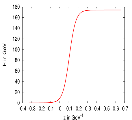
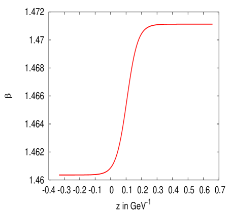
Figure 1: Bubble wall: The higgs vev profile (104) and $\beta$ (105) as a function of $z$.

The wall velocity is taken to be $v_{w}=0.05$ and the plots are evaluated for the first six momenta. The currents $j^{0}$, $j^{0}_{5}$ and the second order term ${j_{5}}^{(2)}$ are evaluated in the plasma frame, thus the expressions are linear in $v_{w}$.

First we will display the dependence on the number of momenta that are used in our fluid Ansatz. Fig. 2 shows that the convergence is already very good for $N=6$, such that it is sufficient to use only the first six momenta.

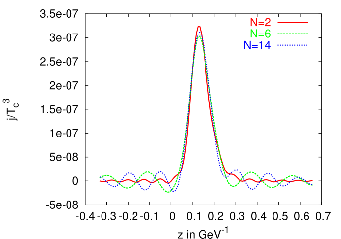
Figure 2: Dependence of the current for a typical source on the number of momenta $N$ used.

Since the higher momenta have a slightly smaller exponential suppression factor but much smaller sources, these contributions become important in the region far away from the source, where the oscillations take place. Mostly the phases of the oscillations are influenced, such that quantitative statements barely change for $N>6$.

The plots Fig. 3 to Fig. 6 show all three currents for the values $\mu_{c}=\{205,220,250,450\}$ GeV and $M_{2}=200$ GeV. For small $\Lambda$, respectively $M_{2}\simeq\mu_{c}$, the solution is oscillating and has rather large amplitudes. These oscillations are, as expected, suppressed for larger values of $\Lambda$ and a local contribution remains. For $\Lambda\sim 20\,T_{c}^{2}\sim T_{c}^{3}L_{w}$ the second order contribution, which shows a weaker dependence on $\Lambda$, begins to dominate. When $\Lambda$ is large, the first order currents are suppressed due to efficient decoherence. In the BAU, the second order terms start to dominate earlier since, for the first order terms, the oscillations and inefficient transport prevent in part an efficient source conversion to baryon asymmetry, while the second order terms are transported more efficiently and without oscillations, such that that give a truly non-local contribution.

The term resulting from the combination $u_{1}\partial_{\mu}u_{2}-u_{2}\partial_{\mu}u_{1}$ is suppressed due to the fact that $\Delta\beta$ is small. In addition, the terms that include $\eta^{3}$ are smaller than the terms including $\eta^{0}$.

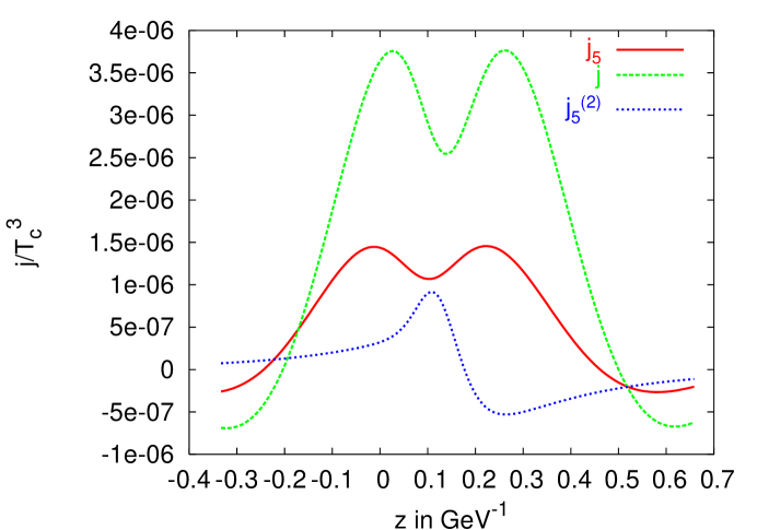
Figure 3: The CP-violating currents of first order $j^{0}$, $j^{0}_{5}$ and of second order ${j_{5}^{0}}^{(2)}$. $M_{2}=200$ GeV. $\mu_{c}=205$ GeV, $\Lambda/T_{c}^{2}\in[0.22,4.0]$.

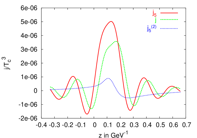
Figure 4: The CP-violating currents of first order $j^{0}$, $j^{0}_{5}$ and of second order ${j_{5}^{0}}^{(2)}$. $M_{2}=200$ GeV. $\mu_{c}=220$ GeV, $\Lambda/T_{c}^{2}\in[0.93,4.2]$.

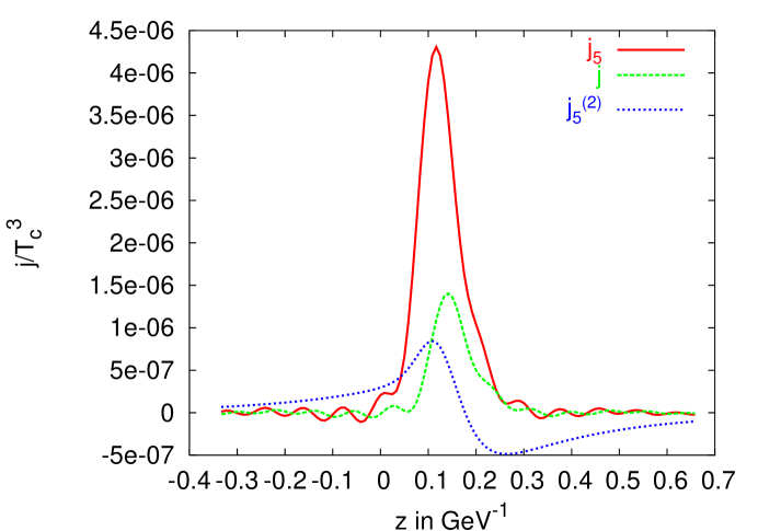
Figure 5: The CP-violating currents of first order $j^{0}$, $j^{0}_{5}$ and of second order ${j_{5}^{0}}^{(2)}$. $M_{2}=200$ GeV. $\mu_{c}=250$ GeV, $\Lambda/T_{c}^{2}\in[2.4,5.1]$.

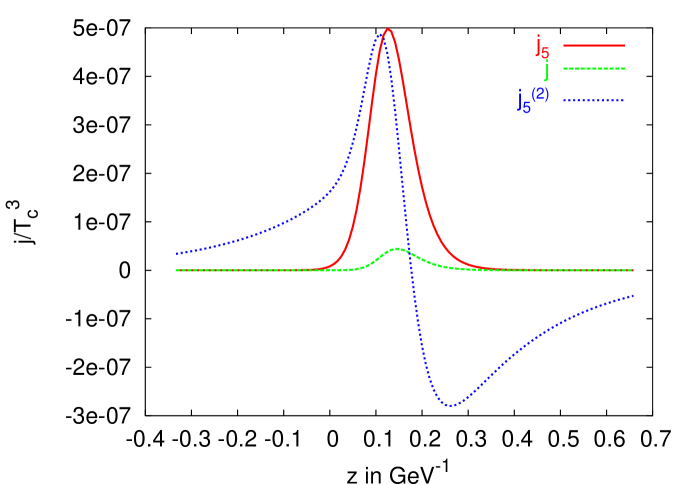
Figure 6: The CP-violating currents of first order $j^{0}$, $j^{0}_{5}$ and of second order ${j_{5}^{0}}^{(2)}$. $M_{2}=200$ GeV. $\mu_{c}=450$ GeV, $\Lambda/T_{c}^{2}\in[18.0,19.2]$.

The axial vector current $j^{0}_{5}$, that is normally the largest contribution to the source, is suppressed for small $\Lambda$ due to the factor $|M_{2}|^{2}-|\mu_{c}|^{2}$ in Eq. (100) and in this region the vector current $j^{0}$ becomes the most important one.

X Discussion and Outlook

In this article we have presented a method to solve Schwinger-Dyson equations for CP-violating densities for mixing fermions in a space time dependent background. The transition to the chiral basis was important for the partial decoupling of the different coefficients in spinor space. The terms that can appear in the kinetic equations written in chiral basis all have the same transformation properties under flavor basis transformations. As an intermediate result, we have obtained the formally exact equations (57), in which only two of the 16 coefficients in spinor space remain coupled to each other.

Next, we have found that the off-diagonal densities exhibit oscillations at lowest order in gradient expansion. Even though they vanish without space-time dependent background, these terms ought to be treated by taking into account oscillations as soon as they are sourced.

In section VI we advance a novel definition of CP violation in kinetic equations with mixing flavors. According to our definition, when kinetic equations with mixing fermions are truncated at first order in gradients, only the inclusion of flavor oscillations (formally expressed through the commutator term) gives raise to nonvanishing CP violation in the diagonal entries of the flavor basis. The same is of course true for the chargino and neutralino sectors in supersymmetric extensions of the Standard Model. This is the main difference between our approach and the approach advocated in literature CarenaQuirosRiottoViljaWagner:1997 ; CarenaMorenoQuirosSecoWagner:2000 ; CarenaQuirosSecoWagner:2002 . Without taking the flavor oscillations into account, the CP-violating densities would stay in the off-diagonal entries even after rotation into the flavor basis.

Our approach to second order diagonal sources (semiclassical force) differs from the treatment advocated in Refs. ProkopecSchmidtWeinstock:2003 ; ProkopecSchmidtWeinstock:2004 ; ClineJoyceKainulainen:2000+2001 . In order to arrive at a local analytic estimate in flavor basis, we have considered the limit of large damping, $\Gamma L\gg 1$. The CP-violating axial current (102) is in this case proportional to the trace in flavor space. The source from semiclassical force in ProkopecSchmidtWeinstock:2003 ; ProkopecSchmidtWeinstock:2004 ; ClineJoyceKainulainen:2000+2001 is calculated in the mass eigenbasis in the limit when $\Gamma L\ll 1$, and it was found to be proportional to the difference of flavor axial densities, ${\rm Tr}(\sigma^{3}j^{3}_{5d})$. Moreover, in our numerical treatment we calculate the source by taking account of both flavor mixing and transport, while the same source has been treated in the literature in the diagonal approximation in the mass eigenbasis.

Apart from the plus contribution, $\propto u_{1}\partial_{\mu}u_{2}+u_{2}\partial_{\mu}u_{1}\equiv\partial_{\mu}(u_{1}u_{2})$, we also found the minus contribution, $u_{1}\partial_{\mu}u_{2}-u_{2}\partial_{\mu}u_{1}$. The plus contribution is sourced by both the first order off-diagonals and by the second order diagonals. The minus term plays an important role in the approach advocated in Refs. CarenaMorenoQuirosSecoWagner:2000 ; CarenaQuirosSecoWagner:2002 , especially near the degeneracy (small $\Lambda$), where it exhibits a resonant enhancement. When compared with our results, in the region of near degeneracy we find a weak enhancement in all contributions to the CP-violating vector current, such that the minus contribution remains subdominant.

By performing a numerical study of fluid equations, we have analysed the CP-violating vector and axial vector currents for a slowly moving wall, and found that, in the nonlocal regime, in which the currents are only weakly damped $\Gamma L_{w}\leq 1$, the first order terms provide a dominant contribution to the CP-violating currents if $\Lambda=m_{i}^{2}-m_{j}^{2}$ ($m_{i}^{2}$ ($i=1,..,N$) denote the mass eigenvalues) is smaller than about $20\,T_{c}^{2}$. Whether this statement remains true with respect to the baryon asymmetry remains unclear, since the oscillations, poor transport and the tracelessness of the first order terms could prevent an efficient production of BAU.

A more comprehensive comparison with the work of Refs. CarenaMorenoQuirosSecoWagner:2000 ; CarenaQuirosSecoWagner:2002 and ProkopecSchmidtWeinstock:2003 ; ProkopecSchmidtWeinstock:2004 ; ClineJoyceKainulainen:2000+2001 , and the explicit calculation of the BAU is postponed to a forthcoming publication.

Appendix A Diagonalization of the Chargino-Higgsino mass matrix

The chargino-higgsino mass matrix is given by

$$m=\left(\begin{array}[]{cc}M_{2}&gH_{2}^{*}\cr gH_{1}^{*}&\mu_{c}\cr\end{array}\right)$$ (106)

The mass matrix $m$ is diagonalized by the biunitary transformation

$$m_{d}=UmV^{\dagger}\,,$$ (107)

with

$$U = \left(\frac{2}{\Lambda(\Lambda+\Delta)}\right)^{\frac{1}{2}}\left(\begin{array}[]{cc}\frac{1}{2}(\Lambda+\Delta)&a\cr-a^{*}&\frac{1}{2}(\Lambda+\Delta)\cr\end{array}\right)$$ (110)

$$a = g(M_{2}H_{1}+\mu_{c}^{*}H_{2}^{*})\,,\qquad\Delta=|M_{2}|^{2}-|\mu_{c}|^{2}-(u_{1}^{2}-u_{2}^{2})\,,\qquad\Lambda=(\Delta^{2}+4|a|^{2})^{\frac{1}{2}}$$

and

$$V = \left(\frac{2}{\bar{\Lambda}(\bar{\Lambda}+\bar{\Delta})}\right)^{\frac{1}{2}}\left(\begin{array}[]{cc}\frac{1}{2}(\bar{\Lambda}+\bar{\Delta})&\bar{a}\cr-\bar{a}^{*}&\frac{1}{2}(\bar{\Lambda}+\bar{\Delta})\cr\end{array}\right)$$ (113)

$$\bar{a} = g(M_{2}^{*}H_{2}^{*}+\mu_{c}H_{1})\,,\qquad\bar{\Delta}=|M_{2}|^{2}-|\mu_{c}|^{2}+(u_{1}^{2}-u_{2}^{2})\,,\qquad\bar{\Lambda}=(\bar{\Delta}^{2}+4|\bar{a}|^{2})^{\frac{1}{2}}=\Lambda$$

where we defined $u_{1,2}=|gH_{1,2}|$. Note that $\bar{a}$ and $\bar{\Delta}$ can be obtained from $a$ and $\Delta$ by the replacements, $M_{2}\leftrightarrow M_{2}^{*}$, $\mu_{c}\leftrightarrow\mu_{c}^{*}$ and $H_{1}\leftrightarrow H_{2}^{\dagger}$, such that $\bar{\Lambda}=\Lambda$, as indicated in (113). The mass eigenvalues-squared are given by

$${m_{d}}_{1/2}^{2}=\frac{1}{2}\big{(}|M_{2}|^{2}+|\mu_{c}|^{2}+(u_{1}^{2}+u_{2}^{2})\big{)}\pm\frac{\Lambda}{2}$$ (114)

and can be calculated quite simply by noting that $Umm^{\dagger}U^{\dagger}=m_{d}^{2}=Vm^{\dagger}mV^{\dagger}$.

References

• (1) G. R. Farrar and M. E. Shaposhnikov, “Baryon Asymmetry Of The Universe In The Minimal Standard Model,” Phys. Rev. Lett.  70 (1993) 2833 [Erratum-ibid.  71 (1993) 210] [arXiv:hep-ph/9305274]. G. R. Farrar and M. E. Shaposhnikov, “Baryon asymmetry of the universe in the standard electroweak theory,” Phys. Rev. D 50 (1994) 774 [arXiv:hep-ph/9305275].
• (2) T. Konstandin, T. Prokopec and M. G. Schmidt, ’‘Axial currents from CKM matrix CP violation and electroweak baryogenesis,” Nucl. Phys. B 679 (2004) 246 [arXiv:hep-ph/0309291].
• (3) M. Joyce, T. Prokopec and N. Turok, “Electroweak baryogenesis from a classical force,” Phys. Rev. Lett.  75 (1995) 1695 [Erratum-ibid.  75 (1995) 3375] [arXiv:hep-ph/9408339].
• (4) M. Joyce, T. Prokopec and N. Turok, “Nonlocal electroweak baryogenesis. Part 1: Thin wall regime,” Phys. Rev. D 53 (1996) 2930 [arXiv:hep-ph/9410281].
• (5) M. Joyce, T. Prokopec and N. Turok, “Nonlocal electroweak baryogenesis. Part 2: The Classical regime,” Phys. Rev. D 53 (1996) 2958 [arXiv:hep-ph/9410282].
• (6) P. Huet and A. E. Nelson, “Electroweak baryogenesis in supersymmetric models,” Phys. Rev. D 53 (1996) 4578 [arXiv:hep-ph/9504427].
• (7) A. T. Davies, C. D. Froggatt and R. G. Moorhouse, “Electroweak Baryogenesis in the Next to Minimal Supersymmetric Model,” Phys. Lett. B 372 (1996) 88 [arXiv:hep-ph/9603388];
• (8) M. Carena, M. Quirós, A. Riotto, I. Vilja and C. E. Wagner, “Electroweak baryogenesis and low energy supersymmetry,” Nucl. Phys. B 503 (1997) 387 [arXiv:hep-ph/9702409].
• (9) J. M. Cline, M. Joyce and K. Kainulainen, “Supersymmetric electroweak baryogenesis in the WKB approximation,” Phys. Lett. B 417 (1998) 79 [Erratum-ibid. B 448 (1998) 321] [arXiv:hep-ph/9708393].
• (10) J. M. Cline and K. Kainulainen, “A new source for electroweak baryogenesis in the MSSM,” Phys. Rev. Lett.  85 (2000) 5519 [arXiv:hep-ph/0002272]; J. M. Cline, M. Joyce and K. Kainulainen, “Supersymmetric electroweak baryogenesis,” JHEP 0007 (2000) 018 [hep-ph/0006119] [Erratum, arXiv:hep-ph/0110031];
• (11) M. Carena, J. M. Moreno, M. Quirós, M. Seco and C. E. Wagner, “Supersymmetric CP-violating currents and electroweak baryogenesis,” Nucl. Phys. B 599 (2001) 158 [arXiv:hep-ph/0011055].
• (12) M. Carena, M. Quirós, M. Seco and C. E. M. Wagner, “Improved results in supersymmetric electroweak baryogenesis,” Nucl. Phys. B 650 (2003) 24 [arXiv:hep-ph/0208043].
• (13) K. Kainulainen, T. Prokopec, M. G. Schmidt and S. Weinstock, “First principle derivation of semiclassical force for electroweak baryogenesis,” JHEP 0106 (2001) 031 [arXiv:hep-ph/0105295].
• (14) K. Kainulainen, T. Prokopec, M. G. Schmidt and S. Weinstock, “Semiclassical force for electroweak baryogenesis: Three-dimensional derivation,” Phys. Rev. D 66 (2002) 043502 [arXiv:hep-ph/0202177].
• (15) S. J. Huber and M. G. Schmidt “Electroweak baryogenesis in a SUSY model with a gauge singlet,” Nucl. Phys. B 606 (2001) 183 [arXiv:hep-ph/0003122]; S. J. Huber and M. G. Schmidt, “SUSY variants of the electroweak phase transition,” Eur. Phys. J. C 10, 473 (1999) [arXiv:hep-ph/9809506].
• (16) T. Prokopec, M. G. Schmidt and S. Weinstock, “Transport equations for chiral fermions to order h-bar and electroweak baryogenesis: Part I,” arXiv:hep-ph/0312110, to be published by Annals of Physics.
• (17) T. Prokopec, M. G. Schmidt and S. Weinstock, “Transport equations for chiral fermions to order h-bar and electroweak baryogenesis: Part II,” arXiv:hep-ph/0406140, to be published by Annals of Physics.
• (18) P. Y. Huet, K. Kajantie, R. G. Leigh, B. H. Liu and L. D. McLerran, “Hydrodynamic stability analysis of burning bubbles in electroweak theory and in QCD,” Phys. Rev. D 48 (1993) 2477 [arXiv:hep-ph/9212224].
• (19) J. M. Moreno, M. Quirós and M. Seco, “Bubbles in the supersymmetric standard model,” Nucl. Phys. B 526 (1998) 489 [arXiv:hep-ph/9801272].
• (20) G. D. Moore and T. Prokopec, “How fast can the wall move? A Study of the electroweak phase transition dynamics,” Phys. Rev. D 52 (1995) 7182 [arXiv:hep-ph/9506475].