Models of Neutrino Masses and Mixings

Abstract

Pocket guide to Terra Incognita of the “Planisphaerium Neutrinorum” (http://www.ba.infn.it/~now2004/) by Eligio Lisi. Includes a survival kit for the $U_{e3}$ territory and a first-aid package for the case of maximal atmospheric mixing angle.

1 INTRODUCTION

By looking at the theoretical developements about neutrino masses and mixing angles of the last few years we may feel uncomfortable, given the large number of existing (and working) models, apparently indicating that, despite the formidable experimental progress, no unique and compelling theoretical picture has emerged so far. To some extent this is true, since we cannot speak of a theory of neutrino or fermion masses. We are still lacking a unifying principle. In a sense, the current theoretical status of fermion masses is comparable to that of weak interactions before the standard electroweak theory was proposed. Several properties of weak processes were well-known, like universality and the V-A character of the charged current. Other properties were conjectured, like the existence of intermediate vector bosons to improve the bad high-energy behaviour of the theory. But it was only with the introduction of the unified electroweak theory that renormalizability and the requirement of SU(2)$\times$ U(1) gauge invariance allowed to determine all interactions between fermions and gauge bosons in terms of only two parameters, the gauge coupling constants of the theory. Unfortunately this is not the case for the interactions between fermions and spin zero particles, responsible for the fermion spectrum. In the electroweak theory, suitably extended to accomodate neutrino oscillations, we may have up to 22 free observable parameters in the flavour sector!

In this talk I will summarize some theoretical aspect of neutrino masses. I will not attempt to review in detail the many existing successful models [1], but I will rather address a number of questions and open problems such as:

• How many light neutrinos exist?

• Why neutrinos are much lighter than charged fermions?

• Which is the absolute neutrino spectrum favoured by the theory?

• What is the most probable range of $U_{e3}$?

• Is the atmospheric mixing angle $\theta_{23}$ maximal?

The tentative answers will illustrate our current ideas and prejudices, which the future experimental results might confirm or upset.

2 HOW MANY LIGHT NEUTRINOS?

We know that, besides the result of the LSND experiment, there are no independent indications in favour of additional, light, sterile neutrinos. The existence of a sterile neutrino is disfavoured by the experiments on both solar and atmospheric neutrinos. Even including the uncertainty on the standard solar model and in particular on the flux of ${}^{8}B$-neutrinos, the SNO results imply that the role of sterile neutrinos in solar oscillations is sub-dominant [2]. Likewise, conversion of atmospheric neutrinos into a sterile component is disfavoured by several independent properties of the data, like for instance the zenith angular dependence of high-energy muons. When a sterile neutrino is added to the three active ones, either in the 2+2 or in the 3+1 scheme, the global fit to oscillation data has a very poor quality. More complicated schemes, such as 3+2, seem to prefer a gap of several eV between the lowest and the highest levels, which is disfavoured by recent cosmological data from the cosmic microwave background radiation and large scale structure [3]. At the moment three active light neutrinos represent the most conservative and plausible possibility, but we should of course wait for an experimental check. If MiniBOONE will confirm the LSND signal, the working hypothesis of three light neutrinos should be abandoned, since not even a CTP violating neutrino spectrum allows to fit all the data with only three flavours [4].

3 WHY NEUTRINOS ARE SO LIGHT?

There are two main theoretical options to describe neutrino masses, depending on whether the total lepton number L is conserved or not. If L is exactly conserved, the smallness of neutrino masses requires a huge hierarchy of Yukawa couplings within the same generation (e.g. $y_{e}/y_{\nu_{e}}>10^{6}$), a fact with no counterpart in the charged fermion sector, where the corresponding gap is at most a factor of about one hundred. Exact conservation of global quantum numbers goes also against several theoretical prejudices. Baryon and lepton numbers are broken by anomalies already in the standard model. They are violated in most of attempts to unify fundamental interactions. Global quantum numbers are also supposed not to survive the quantization of gravity.

Table 1: Bounds from $0\nu\beta\beta$ searches. Experimental values from ref. [5].

experiment	$T_{1/2}$ ($\times 10^{25}$ yr)	$|m_{ee}|$ (eV)
HM(${}^{76}Ge$)	$>1.9$	$<0.35$
IGEX(${}^{76}Ge$)	$>1.6$	$<(0.33\div 1.35)$
Cuore(${}^{130}Te$)	$>5.5\times 10^{-2}$	$<(0.37\div 1.9)$

If L is conserved, one of the most interesting attempts to describe neutrino masses is in the context of models with large extra dimensions [6]. In such models the right-handed neutrino $\nu_{s}(x,y)$ is assumed to have access to both the ordinary four space-time dimensions and to the extra compact dimensions, parametrized by $y$, while all the other fermions are bound to live in a four-dimensional slice of the full space-time, parametrized by $x$. All four-dimensional modes of the Fourier expansion of $\nu_{s}(x,y)$, and in particular the lightest one, $\nu^{(0)}_{s}(x)$, come in the low-energy effective theory with the normalization factor $1/\sqrt{V}$, $V$ being the volume of the extra space:

$$\nu_{s}(x,y)=\frac{1}{\sqrt{V}}\nu^{(0)}_{s}(x)+...~{}~{}~{}~{}~{}.$$ (1)

Therefore the neutrino Yukawa couplings have an extra factor $1/\sqrt{V}$ (in units of a fundamental scale) compared to the other Yukawa couplings and the smallness of the neutrino masses can be explained by the largeness of $V$. At present, there are no experimental indications supporting this idea. In principle, some of the higher modes $\nu^{(n)}_{s}(x)$ might take part in neutrino oscillations, leading to a peculiar oscillation pattern, but present data show that these effects are at most subdominant. Moreover, if L is broken by quantum gravity, in these models the expected effects are huge, since the fundamental scale of gravity in the higher-dimensional theory is also depleted by a factor $1/\sqrt{V}$ compared to the four-dimensional Planck scale.

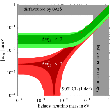
Figure 1: From ref. [7], $90\%$ CL range for $|m_{ee}|$ as function of the lightest neutrino mass, thereby covering all spectra. The darker regions show how the $|m_{ee}|$ range would shrink if the present best-fit values of oscillation parameters were confirmed with negligible error.

If L is not conserved, then the smallness of neutrino masses is explained in terms of the largeness of the scale $\Lambda$ at which L is violated:

$$\frac{(Hl_{i})(Hl_{j})}{\Lambda}=\frac{1}{2}\frac{v^{2}}{\Lambda}\nu_{i}\nu_{j}+...$$ (2)

This scale can be very large, perhaps as large as the grand unification scale. This makes the violation of L theoretically very appealing. Neutrino masses and mixing angles could represent a unique window on otherwise unaccessible energy scales where the relevant description might be in terms of a grand unified theory and where the degrees of freedom required by the see-saw mechanism and by baryogenesis might become manifest.

In principle the scale of L violation can also be much smaller than the electroweak scale, a point of view opposite to the one adopted above. For instance in supersymmetric extensions of the standard model with R-parity breaking from bilinear terms in the superpotential

$$W=\mu_{i}Hl_{i}+...$$ (3)

one neutrino combination becomes massive thanks to a tree-level contribution proportional to $\mu^{2}/m_{SUSY}$ ($\mu_{i}\approx\mu$) where $m_{SUSY}$ is the supersymmetry breaking scale, expected close to the TeV scale. There are two problems with this approach. First, an ad hoc scale $\mu\approx 0.1$ MeV should be introduced in our description of particle interactions, with no independent motivation. Second, the lightest neutrinos get their masses via radiative corrections so that the typical hierarchy is too strong to correctly fit $\Delta m^{2}_{sol}/\Delta m^{2}_{atm}$ and a further fine-tuning of the parameters is needed.

Neutrino oscillations are insensitive to L violation and today the most accurate tests involve the search for neutrinoless double beta decay. The present experiments are sensitive to $|m_{ee}|$, the relevant mass combination, in the sub-eV range, while future searches will push the sensitivity down to about 10 meV, the precise value being unfortunately largely affected by the theoretical uncertainty coming from nuclear matrix elements. The effective mass parameter $|m_{ee}|$ depends on neutrino masses, mixing angles and CP-violating Majorana phases:

$$|m_{ee}| = |\cos^{2}\theta_{13}(\cos^{2}\theta_{12}m_{1}+\sin^{2}\theta_{12}e^{2i\alpha}m_{2})$$ (4)

$$+\sin^{2}\theta_{13}e^{2i\beta}m_{3}|$$

Thus the expected range of $|m_{ee}|$ can be predicted, as a function of the lightest neutrino mass, from the present knowledge of the oscillation parameters $(\Delta m^{2}_{ij},\theta_{ij})$. The results are shown in fig.  1. If the neutrino spectrum is hierarchical with a normal hierarchy, $|m_{ee}|$ is expected to be below the sensitivity of the next generation of experiments. An inverted hierarchy predicts $|m_{ee}|$ in the range ($14\div 53$) meV (90 % C.L.). If neutrinos are degenerate the present bounds on $|m_{ee}|$ give rise to an upper bound on the common neutrino mass of about 1 eV, with a large error related to the poorly known nuclear matrix elements. Thus the discovery of $0\nu\beta\beta$ decay would not only demonstrate that lepton number is violated, but it would also largely help in ordering the neutrino mass spectrum.

4 ABSOLUTE SPECTRUM

The three possible type of neutrino spectrum (degenerate, hierarchical with normal or inverted hierarchy) are all equally viable at the moment. For each of them the theory should face specific problems to achieve a realistic description of the data.

4.1 Degenerate Spectrum

There is a converging evidence that such a spectrum is only possible below the eV scale. The tritium beta decay provides the bound

$$m_{\nu_{e}}\equiv\left(\sum_{i}|U_{ei}|^{2}m_{i}^{2}\right)^{1/2}<2.2~{}{\rm eV}~{}(95\%{\rm C.L.})$$ (5)

where $m_{\nu_{e}}$ effectively coincides with the common value $m\approx m_{i}$ in the degenerate case. If neutrino masses are of Majorana type, the $0\nu\beta\beta$ bound $m<1~{}{\rm eV}$ discussed above also applies. The sum of neutrino masses is strongly limited by recent cosmological observations and, in the ‘standard’ cosmological model, its 95 % C.L. upper limit lies in the range between approximately 0.5 eV and 1.5 eV, the exact value depending on the actual set of data included in the fit [3, 8]. This remarkable bound depends on assumptions characterizing the standard cosmological model and priors in the data analysis, resulting in a large and difficult to size theoretical uncertainty. On a more speculative ground, also the elegant idea of baryogenesis through leptogenesis requires, in its simplest realization, rather light neutrino masses. For instance, in the CP-violating, out-of-equilibrium decay of an heavy right-handed neutrinos (with type I see-saw masses, hierarchical spectrum of right-handed neutrinos and in the so-called strong wash-out regime) the bound $m_{i}<0.15$ eV holds [9]. By relaxing the requirement of hierarchical right-handed neutrinos one can raise the limit up to about 1 eV, but probably not much more in realistic models [10]. Finally, a part of the Heidelberg-Moscow collaboration searching for $0\nu\beta\beta$ in ${}^{76}Ge$, claims a positive signal at the 4$\sigma$ level in their data [11], that include the full statistics from 1990 to 2003. Such a signal is compatible with $|m_{ee}|$ in the range $0.1\div 0.9$ eV and favours a degenerate neutrino spectrum.

If neutrinos are quasi degenerate, the type I see-saw mechanism [12, 13], where Dirac and Majorana mass matrices $m_{D}$ and $M$ are combined according to the relation:

$$m_{\nu}=m_{D}^{T}M^{-1}m_{D}~{}~{}~{}~{},$$ (6)

is of no help. Actually, at first sight it appears quite unplausible to get a degenerate spectrum from eq. (6), unless a fine-tuning or a specific symmetry is invoked to relate $m_{D}$ and $M$. If we abandon eq. (6), we loose the possible connection between neutrino masses and the charged fermion masses, which is nicely present in grand unified theories.

To naturally accommodate a quasi-degenerate neutrino spectrum, it is convenient to rely on some approximate symmetry, directly imposed on the five-dimensional operator of eq. (2). For instance, if the lepton doublets $l_{i}$ $(i=1,2,3)$ transform in flavour space as a three-dimensional vector of an SO(3) rotation symmetry, then in the limit of exact symmetry we have strictly degenerate neutrinos. The theoretical obstacle to promote this (or a similar) zeroth-order approximation into a realistic model is that well-established features of neutrino spectrum, such as the smallness of $\Delta m^{2}_{sol}/\Delta m^{2}_{atm}$, of $\pi/4-\theta_{23}$, of $\pi/4-\theta_{12}$ and of $\theta_{13}$ should entirely arise from symmetry breaking effects, since all these quantities are undetermined in the symmetry limit. At present there is no general consensus on how to unambiguously introduce these breaking effects in the theory.

In some model they are simply added by hand and fitted to the observed parameters, as for instance in the so-called ‘flavour democracy’ approach [14]. This specific model predicts $\sin^{2}2\theta_{23}\approx 0.89$ and is currently disfavoured by the 2$\sigma$ bound $\sin^{2}2\theta_{23}>0.90$.

In other models the breaking effects are produced by the dynamics of an underlying symmetry breaking sector. This dynamics is highly non-trivial and requires a special misalignment between breaking effects in the neutrino and in the charged lepton sector, in order to give rise to the large observed mixing angles [15].

Finally, to avoid a full-fledged theory of breaking terms, we can assume that the neutrino mass matrix is anarchical (A) [16] with matrix elements being random, order-one, coefficients in units of a common mass scale $m$:

$$m_{\nu}=\left(\begin{array}[]{ccc}O(1)&O(1)&O(1)\\ O(1)&O(1)&O(1)\\ O(1)&O(1)&O(1)\end{array}\right)m~{}~{}~{}~{}~{}.$$ (7)

This speculative scenario has the interesting property that, on a statistical basis, a moderate hierarchy for $\Delta m^{2}_{sol}/\Delta m^{2}_{atm}$ can be produced by the see-saw mechanism and that large mixing angles are naturally expected. This is good for the solar and atmospheric angles (although $\theta_{23}=\pi/4$ would be accidental), but less good for $\theta_{13}$, which is thus expected very close to the present experimental bound.

4.2 Inverted Hierarchy

At the moment the most convincing model for an inverted neutrino hierarchy (IH) is the one based on the leading order texture:

$$m_{\nu}=\left(\begin{array}[]{ccc}0&a&b\\ a&0&0\\ b&0&0\end{array}\right)~{}~{}~{}~{}~{},$$ (8)

obtained, for instance, by asking invariance under $L_{e}-L_{\mu}-L_{\tau}$. Nice features of the above texture are $\theta_{13}=0$ and $\tan\theta_{23}=-b/a$ (adjustable to 1 by taking $b=-a$). A difficulty arises from the prediction of the solar angle, $\theta_{12}=45^{0}$, out by about 6$\sigma$ from the experimental value ($\approx 33^{0}\pm 2^{0}$).

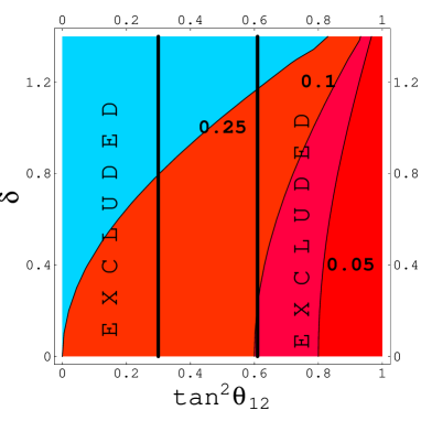
Figure 2: Contours of $|U_{e3}|$ in the plane $(\tan^{2}\theta_{12},\delta_{CP})$. The two vertical lines represent the present 3$\sigma$ lower and upper limit on $\tan^{2}\theta_{12}$ (see eq. (9)).

We may think to fix this problem by turning on small breaking terms (filling the zeros in the above texture) also needed to reproduce $\Delta m^{2}_{sol}\neq 0$. However, barring fine-tuning, these breaking terms obey to the approximate relation $1-\tan^{2}\theta_{12}\approx O(\Delta m^{2}_{sol}/\Delta m^{2}_{atm})$, which is off by a factor $>10$ [17]:

$$1-\tan^{2}\theta_{12} = (0.39\div 0.70)~{}(3\sigma)$$ (9)

$$\Delta m^{2}_{sol}/\Delta m^{2}_{atm} = (0.024\div 0.060)~{}(3\sigma)~{}~{}.$$ (10)

This difficulty is shared by many models, such as the above mention flavour democracy model or, more generally, models with a pseudo-Dirac structure in the 12 sector:

$$\left(\begin{array}[]{cc}0&1\\ 1&0\end{array}\right)~{}~{}~{}~{}~{}.$$ (11)

The problem can be solved by taking into account the contribution to the mixing angles coming from the charged lepton sector [18, 19]. The mixing matrix is given by $U_{PMNS}=U_{e}^{\dagger}U_{\nu}$, where $U_{\nu}$ and $U_{e}$ come from the diagonalization of the neutrino and charged lepton mass matrix, respectively. By adopting a standard parametrization for $U_{\nu,e}=U^{\nu,e}_{23}\cdot U^{\nu,e}_{13}\cdot U^{\nu,e}_{12}$, we can absorb $U^{e}_{23}$ into $U_{\nu}$ and, by assuming $\theta^{\nu}_{23}=\pi/4$, we have a bimaximal mixing in the neutrino sector, to start with. Then we can compute the effect of small angles $\theta^{e}_{12}$ and $\theta^{e}_{13}$ on $U_{PMNS}$, obtaining:

$$1-\tan^{2}\theta_{12} = 2\sqrt{2}~{}Re(u+v)$$ (12)

$$|U_{e3}| = \frac{1}{\sqrt{2}}|u-v|$$ (13)

$$\delta_{CP} = arg(u-v)$$ (14)

$$\tan^{2}\theta_{23} = 1$$ (15)

where $u$ and $v$ are complex numbers, $(|u|,|v|)\equiv(\sin\theta^{e}_{12},\sin\theta^{e}_{13})$ and the above results hold to first order in $(|u|,|v|)\ll 1$. By analogy with the quark sector, we may tentatively assume:

$$|v|\ll|u|\approx\lambda\approx 0.22~{}~{}~{}~{}~{},$$ (16)

and we get:

$$|U_{e3}| \approx \frac{(1-\tan^{2}\theta_{12})}{4\cos\delta_{CP}}$$ (17)

$$1-\tan^{2}\theta_{12} \approx 2\sqrt{2}~{}\lambda\approx 0.6~{}~{}~{}~{}~{}.$$ (18)

We see that $\theta_{12}$ is indeed corrected by the right amount (also suggesting an intriguing complementarity between $\theta_{12}$ and $\lambda$ [20]) but, at the same time, a non-vanishing $|U_{e3}|$ is produced. Actually, from equation (17), a rather large value of $|U_{e3}|$ is expected. In fig. 2 a contour plot of $|U_{e3}|$ in the plane $(\tan^{2}\theta_{12},\delta_{CP})$ shows that in most of the available parameter space, where we keep assuming $|v|\ll|u|$, $|U_{e3}|$ is larger that 0.1. This model of inverse hierarchy can be realized both within and without the see-saw mechanism.

4.3 Normal Hierarchy

The interesting feature of a hierarchical neutrino spectrum with normal hierarchy is the central role played by the see-saw mechanism, at variance with inverse hierarchy where such a mechanism is an option and with the degenerate case where it may even represent an obstacle. In the so-called flavour basis, where the charged leptons are diagonal, the condition for a hierarchical neutrino spectrum and large atmospheric and solar mixing angles is that the 23 block of the neutrino mass matrix has comparable matrix elements with a suppressed determinant. In the context of the see-saw mechanism there are two natural possibilities to met this condition.

• The see-saw mechanism is dominated by a single, relatively ‘light’ right-handed neutrino, equally coupled to $\nu_{\mu}$ and $\nu_{\tau}$ [21];

• The mass matrices $m_{e}$ and/or $m_{D}$ (with the convention ($\bar{R}m_{e/D}L$) have an approximate ‘lopsided’ structure [22]:

  $$\left(\begin{array}[]{ccc}0&0&0\\ 0&0&0\\ 0&a&b\end{array}\right)~{}~{}~{}~{}~{}.$$ (19)

A typical texture for neutrinos with normal hierarchy, as arising in models with U(1) flavour symmetry, is

$$m_{\nu}=\left(\begin{array}[]{ccc}\epsilon^{2}&\epsilon&\epsilon\\ \epsilon&1&1\\ \epsilon&1&1\end{array}\right)m~{}~{}~{}~{}~{},$$ (20)

where $\epsilon<1$ is the symmetry breaking parameter and all entries are given up to unknown O(1) coefficients. The angle $\theta_{13}$ is of order $\epsilon$. A hierarchical spectrum and a large solar mixing angle require that the determinant of the 23 block is of order $\epsilon$. This may happen accidentally, and we may call the corresponding models semi-anarchical (SA), or thanks to one of the two possibilities mentioned above (H models). Both these possibilities can be realized in the context of a grand unified theory, where they are compatible with the observed smallness of the quark mixing. In particular, the large mixing angle among charged fermions expected in the lopsided texture corresponds in SU(5) to a mixing between right-handed down quarks and, as such, is not directly manifest in weak processes.

5 ESTIMATES OF $U_{e3}$

It is quite difficult to arrange for a tiny $U_{e3}$ in a realistic model of neutrino masses. By tiny here I mean well below 0.05, which approximately corresponds to the square $\lambda^{2}$ of the Cabibbo angle. The range between 0.05 and the present upper bound will be presumably explored in about ten years from now and it will not require a neutrino factory program.

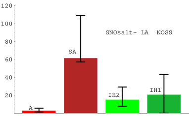
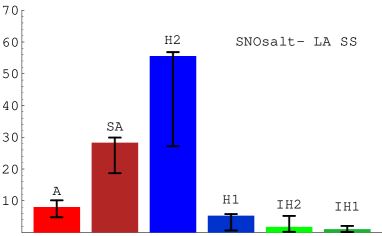
Figure 3: Relative success rates of models with U(1) flavour symmetry, analyzed both without (NOSS) and within (SS) the see-saw mechanism. The sum of the rates has been normalized to 100. The results correspond to the optimized values of $\epsilon$: $1$, $0.2$, $0.25$, $0.25$, for the models A, SA, IH2, IH1 (NOSS case) and $1$, $0.25$, $0.12$, $0.2$, $0.45$, $0.25$ for the models A, SA, H2, H1, IH2, IH1 (SS case). The error bars represent the linear sum of the systematic error and the statistical error. For details, see ref. [23].

We have already seen that in inverted hierarchy the leading order prediction $U_{e3}=0$ is substantially modified by the corrections coming from the charged lepton sector, so that, barring cancellation, we expect (see eqs. (9,17)):

$$|U_{e3}|>\frac{(1-\tan^{2}\theta_{12})}{4}\approx(0.10\div 0.18)~{}[3\sigma]~{}~{},$$ (21)

which is within a factor of two from the present bound. For a normal hierarchy, we may estimate $U_{e3}$ from the approximate relation

$$U_{e3}\approx\sin\theta^{\nu}_{13}-\sin\theta_{23}\sin\theta^{e}_{12}~{}~{}~{}~{}~{},$$ (22)

which holds under the plausible assumptions that both the contributions from the neutrino and the charged lepton sectors are small (i.e. no cancellations between large terms) and that $\sin\theta^{e}_{12}$ dominates over $\sin\theta^{e}_{13}$. In ‘typical’ models $\sin\theta^{\nu}_{13}$ is of order $\sin\theta_{12}\sqrt{\Delta m^{2}_{sol}/\Delta m^{2}_{atm}}$, which lies in the range $(0.03\div 0.3)$ (by allowing for a 3$\sigma$ experimental uncertainty and by modeling through factors 1/2 and 2 the theoretical uncertainty, here and in the following estimates). The contribution from the charged leptons is typically of order $\sin\theta_{23}\sqrt{m_{e}/m_{\mu}}\approx(0.02\div 0.1)$. Again, excluding cancellations between the two contributions we find that $U_{e3}$ cannot be tiny. (If we used the analogue of eq. (22) to estimate $V_{ub}$ from $V_{cb}\approx\lambda^{2}$ and $V_{us}\approx\lambda$, we would get $V_{ub}\approx\lambda^{3}$.) In models of degenerate neutrinos everything is determined by breaking terms and we should proceed through examples. For instance, in a model where $\Delta m^{2}_{sol}$ and $U_{e3}$ are determined by renormalization group evolution, $U_{e3}\approx\sqrt{\Delta m^{2}_{sol}/2\Delta m^{2}_{atm}}\approx(0.04\div 0.4)$. In the flavour democracy model, $U_{e3}\approx\sqrt{2m_{e}/3m_{\mu}}\approx(0.03\div 0.1)$. In the anarchical approach, $U_{e3}\approx O(1)$.

In a specific class of models a more quantitative analysis can be performed. For instance, models with a U(1) flavour symmetry are flexible enough to cover all possible type of neutrino spectrum. By varying the U(1) charge assignment we can get neutrino mass matrices of the following structure:

$$m_{\nu} = \left(\begin{array}[]{ccc}\epsilon^{2}&\epsilon&\epsilon\\ \epsilon&1&1\\ \epsilon&1&1\end{array}\right)m~{}~{}~{}~{}~{}$$

$${\rm or}$$

$$m_{\nu} = \left(\begin{array}[]{ccc}\epsilon^{2}&1&1\\ 1&\epsilon^{2}&\epsilon^{2}\\ 1&\epsilon^{2}&\epsilon^{2}\end{array}\right)m~{}~{}~{}~{}~{},$$ (30)

where all matrix elements are up to unknown O(1) coefficients, which the U(1) symmetry is unable to predict, and $\epsilon$ is a free parameter. If $\epsilon=1$, these textures reproduce the A model. Otherwise, $\epsilon<1$ represents the order parameter of U(1) symmetry breaking. In this case, eq. (5) gives rise to both the SA and the H models, depending on whether the determinant of the 23 block is typically of order 1 or $\epsilon$, respectively. Eq. (30) corresponds to the IH model. Given the presence of unknown O(1) parameters, these textures can only predict masses and mixing angles on a statistical basis [23]. In practice the O(1) parameters are taken as complex random numbers, with a given initial distribution. The corresponding predictions are compared with the 3$\sigma$ experimental windows:

$$0.018< |\Delta m^{2}_{sol}/\Delta m^{2}_{atm}| <0.053$$

$$0.30< \tan^{2}\theta_{12} <0.64$$

$$0.45< \tan^{2}\theta_{23} <2.57$$ (31)

$$|U_{e3}| <0.23~{}~{}~{}~{}~{},$$

and a success rate is evaluated. The procedure is iterated and the parameter $\epsilon$ is optimized to maximize the success rate of each model. In fig. 3 the results of such an optimization are displayed and we can see that models possessing some degree of order are preferred over models based on structure-less mass matrices. Also, for SA, H, and IH models, an expansion parameter $\epsilon$ numerically close to the Cabibbo angle is needed (see figure caption) to better account for the smallness of $\Delta m^{2}_{sol}/\Delta m^{2}_{atm}$ and of $|U_{e3}|$.

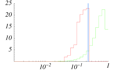
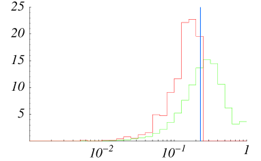
Figure 4: Distribution of $|U_{e3}|$ [24] for the models A (top) and SA (bottom), with see-saw mechanism, before (green, light) and after (red, dark) the selection made by the experimental cuts in eq. (31). The vertical line shows the present experimental bound.

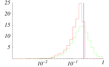
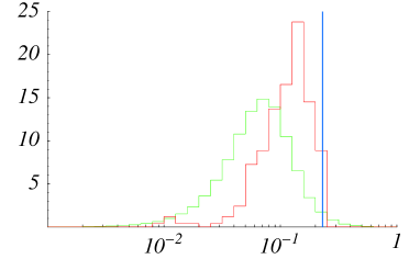
Figure 5: Distribution of $|U_{e3}|$ [24] for the models H2 with see-saw mechanism (top) and IH without see-saw mechanism (bottom), before (green, light) and after (red, dark) the selection made by the experimental cuts in eq. (31). The vertical line shows the present experimental bound.

For the successful models we can finally analyze the distributions of $|U_{e3}|$ [24], some of which are displayed in fig. 4 and fig. 5. Such distributions, which clearly have just the purpose of providing a rough orientation, show that a value of $|U_{e3}|$ close to the present experimental upper bound is preferred, with ‘statistical’ tails extending down to, but not below, the percent level. These tails are shorter for the A and IH models.

If ‘normal’ models are likely to predict $|U_{e3}|$ at or above the $\lambda^{2}$ level, we may ask if ‘special’ models exist, where $|U_{e3}|\ll\lambda^{2}$. First we can analyze the case of models where a small $|U_{e3}|$ does not arise from the cancellation of comparable contributions. In this case $|U_{e3}|$ is approximately given by eq. (22) and both $\theta^{\nu}_{13}\ll\lambda^{2}$ and $\theta^{e}_{12}\ll\lambda^{2}$ are required in order to obtain a tiny $|U_{e3}|$. It is relatively easy to get $\theta^{\nu}_{13}=0$ in a symmetry limit. For instance, the textures in eq. (5,30), implied by U(1) flavour symmetries, predict $\theta^{\nu}_{13}=0$ when the symmetry breaking parameter $\epsilon$ is set to zero. However, turning $\epsilon$ on, we get $\theta^{\nu}_{13}\approx\sqrt{\Delta m^{2}_{sol}/\Delta m^{2}_{atm}}$ and $\theta^{\nu}_{13}\approx\Delta m^{2}_{sol}/\Delta m^{2}_{atm}$, for (5) and (30), respectively. For a more efficient suppression of $\theta^{\nu}_{13}$ we can look for a symmetry that guarantees $\theta^{\nu}_{13}=0$ and that, in the neutrino sector, does not need any correction term. For instance a $Z_{2}$ symmetry exchanging the muon and tau SU(2) doublets implies:

$$m_{\nu}=\left(\begin{array}[]{ccc}x&y&y\\ y&w&z\\ y&z&w\end{array}\right)~{}~{}~{}~{}~{},$$ (32)

which in turn leads to $\theta^{\nu}_{23}=\pi/4$ and $\theta^{\nu}_{13}=0$ and allows to fit $\theta^{\nu}_{12}$ and $\Delta m^{2}_{sol}/\Delta m^{2}_{atm}$ by adjusting the free parameters $x$, $y$, $z$ and $w$. However, in realistic models such a symmetry is expected to be broken by O(1) effects in the charged lepton sector to account for $m_{\mu}\ll m_{\tau}$. Moreover, in general it is difficult to accommodate $\theta^{e}_{12}\ll\lambda^{2}$ at the same time. As a consequence the previous estimates of $U_{e3}$ probably apply also to this class of models [25].

Alternatively, $|U_{e3}|\ll\lambda^{2}$ can occur as the result of a compensation between O(1) terms. This may happen in models where the lepton mixing angles come entirely from the charged lepton sector and $U_{e3}$ is given by:

$$U_{e3}=\sin\theta^{e}_{12}\sin\theta^{e}_{23}-\cos\theta^{e}_{12}\sin\theta^{e}_{13}\cos\theta^{e}_{23}~{}~{}~{}~{}~{}.$$ (33)

In a particular model of this class it is indeed possible to arrange $U_{e3}\approx m_{e}/m_{\tau}\approx\lambda^{4}$, even though the construction is considerably more complicated than in ‘normal’ models [19].

In summary, it is reasonable to expect that most of the plausible range for $|U_{e3}|$ will be explored in about ten years from now. Without further information, discovery of $|U_{e3}|$ in the range $(0.10\div 0.23)$ will not favour a particular model and/or a particular type of spectrum. A relatively small, but still sizeable $|U_{e3}|$, between 0.05 and 0.10, is difficult to reconcile with anarchy and with inverse hierarchy, in its simplest version. If $|U_{e3}|\ll 0.05$ then a very narrow, but not empty, subset of the existing models would be selected. The interested reader can compare the above estimates with those of the recent literature [26].

6 IS $\theta_{23}$ MAXIMAL ?

The present best value of $\theta_{23}$ is very close to $45^{0}$, with a still large 3$\sigma$ uncertainty:

$$35.7^{0}<\theta_{23}<55.6^{0}~{}~{}~{}.$$ (34)

Since the determination of $\theta_{23}$ is mainly due to the measurement of the $\nu_{\mu}$ survival probability and $\delta P_{\mu\mu}\approx\delta(\sin^{2}2\theta_{23})\approx 4\delta(\Delta^{2})$ $(\Delta\equiv\theta_{23}-\pi/4)$, it will be very difficult in the future to improve the experimental precision on $\theta_{23}$. To achieve a reduction of the error by a factor of two, we will probably need superbeams and a time scale of about ten years [27]. Nevertheless future data might confirm the preference for a maximal $\theta_{23}$ and motivate the search for a natural explanation of such a peculiar feature of lepton mixing. The natural question that comes to mind is if $\theta_{23}=\pi/4$ can be understood in some symmetry limit of the flavour sector. If true, this could be of great help in our search for a unifying principle. Several observable quantities can be understood via exact or approximate symmetries of particle interactions, as for example the photon mass whose vanishing is guaranteed by the U(1) electromagnetic gauge invariance or as the electroweak $\rho$ parameter, which an approximate custodial symmetry requires to be close to one.

I will conclude this presentation by illustrating a perhaps not well-known and to some extent counterintuitive property. Contrary to expectations, a maximal mixing angle $\theta_{23}$ can never arise in a symmetry limit of whatever flavour symmetry (global or local, continuous or discrete), provided such a symmetry is only broken by small effects in the real world, as we expect for a meaningful symmetry. This result does not necessarily have a negative impact on the theory. The immediate implication is that, in the context of a sensible flavour symmetry, $\theta_{23}=\pi/4$ can only arise as a breaking effect. Therefore, if really $\theta_{23}$ is maximal or nearly maximal in nature, our description of lepton mixing will be severely constrained and in any model of maximal atmospheric mixing based on a symmetry approach, both the underlying symmetry and the symmetry breaking sector should be carefully chosen.

I give here a shortcut to the full argument. Consider the charged lepton mass matrix:

$$m_{l}=m^{0}_{l}+...~{}~{}~{},$$ (35)

where $m^{0}_{l}$ represents the limit of an exact flavour symmetry F and dots are the symmetry breaking effects that vanish when F is exact. We should distinguish two cases. The first case is when $m^{0}_{l}$ has rank less or equal to one. This is true for most of realistic flavour symmetries. In a suitable basis:

$$m^{0}_{l}=\left(\begin{array}[]{ccc}0&0&0\\ 0&0&0\\ 0&0&m_{\tau}\end{array}\right)~{}~{}~{}~{}~{},$$ (36)

and only the $\tau$ lepton possibly has a non-vanishing mass in the symmetry limit. Electron and muon masses arise as symmetry breaking effects. It is clear from eq. (36) that $\theta^{e}_{12}$ is undetermined in this limit. Therefore

$$\tan\theta_{23}=\tan\theta^{\nu}_{23}\cos\theta^{e}_{12}+\frac{\tan\theta^{\nu}_{13}}{\cos\theta^{\nu}_{23}}\sin\theta^{e}_{12}~{}~{}~{}~{}~{}$$ (37)

is also undetermined, no matter what is the leading neutrino mass matrix. When small breaking terms are turned on, both $m_{l}^{0}$ and $m_{\nu}^{0}$ are modified and, to obtain a maximal atmospheric mixing angle, we need a conspiracy between the breaking effects in the neutrino and in the charged lepton sector. For instance, in the limit of an exact SO(3) flavour symmetry under which the lepton doublets transform as a vector, we can have:

$$m^{0}_{\nu}=\left(\begin{array}[]{ccc}1&0&0\\ 0&1&0\\ 0&0&1\end{array}\right)m~{}~{}~{}~{}~{},$$ (38)

$$m^{0}_{l}=\left(\begin{array}[]{ccc}0&0&0\\ 0&0&0\\ 0&0&0\end{array}\right)~{}~{}~{}~{}~{},$$ (39)

and a possible breaking giving rise to a maximal $\theta_{23}$ is described by small terms $x,x^{\prime},y,y^{\prime}\ll 1$ such that:

$$m^{0}_{\nu}=\left(\begin{array}[]{ccc}1&0&0\\ 0&1+x^{\prime}&0\\ 0&0&1+x\end{array}\right)m~{}~{}~{}~{}~{},$$ (40)

$$m^{0}_{l}=\left(\begin{array}[]{ccc}0&0&0\\ 0&y^{\prime}&-y^{\prime}\\ 0&y&y\end{array}\right)\frac{v}{\sqrt{2}}~{}~{}~{}~{}~{}.$$ (41)

The second possibility is that $m^{0}_{l}$ has rank larger or equal than two:

$$m^{0}_{l}=\left(\begin{array}[]{ccc}0&0&0\\ 0&m_{\mu}&0\\ 0&0&m_{\tau}\end{array}\right)~{}~{}~{}~{}~{}.$$ (42)

In this case $\theta_{23}=\pi/4$ is possible in the symmetry limit, but we are left with the problem of explaining why $m_{\mu}\ll m_{\tau}$. Since both masses are non-vanishing in the symmetry limit, generically large O(1) breaking effects are needed to correct the charged lepton spectrum. This is precisely the kind of symmetry we have excluded from our considerations since O(1) corrections can easily upset the result $\theta_{23}=\pi/4$.

7 CONCLUSION

Many questions about the nature of the neutrino mass spectrum are still unanswered. The most conservative theoretical approach is in terms of three light neutrinos whose lightness is naturally described by L violation at a large energy scale. The absolute spectrum is an open experimental problem, though several theoretical (and speculative) properties like type I see-saw, leptogenesis, relationship with other fermion masses in GUTs favour, in their simplest realization, a hierarchical spectrum. At present both normal and inverse hierarchy are equally viable, but in the future tests of $\tan^{2}\theta_{12}$ and $|U_{e3}|$ might constrain more strongly the inverse hierarchy scheme. In most of known models $|U_{e3}|$ is not much smaller than the square of the Cabibbo angle. A tiny $|U_{e3}|$ is possible in principle but needs the construction of an ad hoc model. It is true that the hierarchies among observed quantities are less pronounced in the lepton than in the quark sector. Nevertheless an expansion parameter numerically close to the Cabibbo angle largely helps in reproducing the relative smallness of $\Delta m^{2}_{sol}/\Delta m^{2}_{atm}$ and of $|U_{e3}|$. Finally a nearly maximal $\theta_{23}$ represents a perhaps premature, but quite interesting challenge, which would strongly constrain the present theoretical framework.

References

- [1] For a review of models and for a more complete list of references, see G. Altarelli and F. Feruglio, New J. Phys. 6 (2004) 106.
- [2] J. N. Bahcall and C. Pena-Garay, JHEP 0311 (2003) 004.
- [3] S. Hannestad and G. Raffelt, JCAP 0404 (2004) 008; P. Crotty, J. Lesgourgues and S. Pastor, Phys. Rev. D 69 (2004) 123007.
- [4] S. Pakvasa and J. W. F. Valle, Proc. Indian Natl. Sci. Acad. 70A (2004) 189.
- [5] S. R. Elliott and J. Engel, J. Phys. G 30 (2004) R183.
- [6] F. Feruglio, proceedings of International Europhysics Conference on High-Energy Physics (HEP 2003), Aachen, Germany, 17-23 Jul 2003, arXiv:hep-ph/0401033.
- [7] F. Feruglio, A. Strumia and F. Vissani, Nucl. Phys. B 637 (2002) 345 [Addendum-ibid. B 659 (2003) 359].
- [8] S. Hannestad, arXiv:hep-ph/0404239; G. L. Fogli, E. Lisi, A. Marrone, A. Melchiorri, A. Palazzo, P. Serra and J. Silk, arXiv:hep-ph/0408045.
- [9] G. F. Giudice, A. Notari, M. Raidal, A. Riotto and A. Strumia, Nucl. Phys. B 685 (2004) 89; W. Buchmuller, P. Di Bari and M. Plumacher, arXiv:hep-ph/0401240;
- [10] T. Hambye, Y. Lin, A. Notari, M. Papucci and A. Strumia, Nucl. Phys. B 695 (2004) 169 [arXiv:hep-ph/0312203].
- [11] H. V. Klapdor-Kleingrothaus, I. V. Krivosheina, A. Dietz and O. Chkvorets, Phys. Lett. B 586 (2004) 198
- [12] P. Minkowski, Phys. Lett. B 67 (1977) 421.
- [13] T. Yanagida, in Proc. of the Workshop on Unified Theory and Baryon Number in the Universe, KEK, March 1979; S. L. Glashow, in “Quarks and Leptons”, Cargèse, ed. M. Lévy et al., Plenum, 1980 New York, p. 707; M. Gell-Mann, P. Ramond and R. Slansky, in Supergravity, Stony Brook, Sept 1979; R. N. Mohapatra and G. Senjanovic, Phys. Rev. Lett. 44 (1980) 912.
- [14] H. Fritzsch, Z.Z. Xing, Phys. Lett. B372, 265 (1996); H. Fritzsch, Z.Z. Xing, Phys. Lett. B440, 313 (1998); H. Fritzsch, Z.Z. Xing, Prog. Part. Nucl. Phys. 45, 1 (2000);
- [15] C. Wetterich, Phys. Lett. B 451, 397 (1999); R. Barbieri, L. J. Hall, G. L. Kane and G. G. Ross, hep-ph/9901228.
- [16] L. J. Hall, H. Murayama and N. Weiner, Phys. Rev. Lett. 84, 2572 (2000); N. Haba and H. Murayama, Phys. Rev. D 63, 053010 (2001);
- [17] G. L. Fogli, E. Lisi, A. Marrone, D. Montanino, A. Palazzo and A. M. Rotunno, eConf C030626 (2003) THAT05 [arXiv:hep-ph/0310012]; M. Maltoni, T. Schwetz, M. A. Tortola and J. W. F. Valle, arXiv:hep-ph/0405172.
- [18] P. H. Frampton, S. T. Petcov and W. Rodejohann, Nucl. Phys. B 687 (2004) 31; A. Romanino, Phys. Rev. D 70 (2004) 013003.
- [19] G. Altarelli, F. Feruglio and I. Masina, Nucl. Phys. B 689 (2004) 157.
- [20] M. Raidal, arXiv:hep-ph/0404046; H. Minakata and A. Y. Smirnov, arXiv:hep-ph/0405088.
- [21] S. F. King, Phys. Lett. B439 (1998) 350;
- [22] K. S. Babu and S. M. Barr, Phys. Lett. B 381 (1996) 202; C. H. Albright and S. M. Barr, Phys. Rev. D 58, 013002 (1998); C. H. Albright, K. S. Babu and S. M. Barr, Phys. Rev. Lett. 81, 1167 (1998); G. Altarelli and F. Feruglio, Phys. Lett. B 439, 112 (1998); G. Altarelli and F. Feruglio, JHEP 9811, 021 (1998); P. H. Frampton and A. Rasin, Phys. Lett. B 478, 424 (2000).
- [23] G. Altarelli, F. Feruglio and I. Masina, JHEP 0301 (2003) 035.
- [24] These distributions have been kindly worked out by Isabella Masina.
- [25] W. Grimus, A. S. Joshipura, S. Kaneko, L. Lavoura, H. Sawanaka and M. Tanimoto, arXiv:hep-ph/0408123; R. N. Mohapatra, arXiv:hep-ph/0408187.
- [26] E. K. Akhmedov, G. C. Branco and M. N. Rebelo, Phys. Rev. Lett. 84 (2000) 3535; R. Barbieri, T. Hambye and A. Romanino, JHEP 0303 (2003) 017; M. C. Chen and K. T. Mahanthappa, Int. J. Mod. Phys. A 18 (2003) 5819; A. Ibarra and G. G. Ross, Phys. Lett. B 575 (2003) 279; R. F. Lebed and D. R. Martin, Phys. Rev. D 70 (2004) 013004; A. Joshipura, talk at NOON 2004, February 11-15, 2004, Odaiba, Tokyo, Japan. Slides abvailable at the site http://www-sk.icrr.u-tokyo.ac.jp/noon2004/
- [27] P. Huber, M. Lindner, M. Rolinec, T. Schwetz and W. Winter, arXiv:hep-ph/0403068.