$B\rightarrow X_{d}\ell^{+}\ell^{-}$ in a CP softly broken two Higgs doublet model

Abstract

We study the differential branching ratio, forward-backward asymmetry, CP-violating asymmetry, CP-violating asymmetry in the forward-backward asymmetry and polarization asymmetries of the final lepton in the $B\rightarrow X_{d}\,\ell^{+}\ell^{-}$decays in the context of a CP softly broken two Higgs doublet model. We analyze the dependencies of these observables on the model parameters by paying a special attention to the effects of neutral Higgs boson (NHB) exchanges and possible CP violating effects. We find that NHB effects are quite significant for the $\tau$ mode. The above-mentioned observables seems to be promising as a testing ground for new physics beyond the SM, especially for the existence of the CP-violating phase in the theory.

PACS numbers: 12.60.Fr, 13.20.He

1 Introduction

Although CP violation is one of the most fundamental phenomena in particle physics it is still one of the the least tested aspects of the the Standard Model (SM). Before the start of the B factories, CP violation has only been measured in the kaon system. Very recently, the observation of CP violation in the B-meson system have been reported by the $e^{+}e^{-}$ B factories [1] providing the the first test of the SM CP violation. In the near future, more experimental tests will be possible at the B factories and possible deviations from the SM predictions will provide important clues about physics beyond it. This situation makes the search for CP violation in B decays highly interesting.

Interest in CP violation is not limited to particle physics; it plays an important role in cosmology, too. One of the necessary conditions to generate the matter-antimatter asymmetry observed in the Universe is -in addition to baryon number violation and deviations from the thermal equilibrium- that the elementary interactions have to violate CP. In the SM the only source of CP violation is the complex Cabibbo-Kobayashi-Maskawa (CKM) matrix elements which appears too weak to drive such an asymmetry [2], giving a strong motivation to search for new physics. In many cases, extensions of the SM such as the Two Higgs Doublet Model (2HDM) or the supersymmetric extensions of the SM are able to supply the new sources of CP violation, providing an opportunity to investigate the new physics by analyzing the CP violating effects.

Being a FCNC process, $B\rightarrow X_{s,d}\,\ell^{+}\ell^{-}$ decays provide the most reliable testing grounds for the SM at the loop level and they are also sensitive to new physics. In addition, $B\rightarrow X_{d}\,\ell^{+}\ell^{-}$mode is especially important in the CKM phenomenology. In case of the $b\rightarrow s\ell^{+}\ell^{-}$ decays, the matrix element receives a combination of various contributions from the intermediate $t$, $c$ or $u$ quarks with factors $V_{tb}V^{*}_{ts}\sim\lambda^{2}$, $V_{cb}V^{*}_{cs}\sim\lambda^{2}$ and $V_{ub}V^{*}_{us}\sim\lambda^{4}$, respectively, where $\lambda=\sin\theta_{C}\cong 0.22$. Since the last factor is extremely small compared to the other two we can neglect it and this reduces the unitarity relation for the CKM factors to the form $V_{tb}V^{*}_{ts}+V_{cb}V^{*}_{cs}\approx 0$. Hence, the matrix element for the $b\rightarrow s\ell^{+}\ell^{-}$ decays involve only one independent CKM factor so that CP violation would not show up. On the other hand, as pointed out before [3, 4], for $b\rightarrow d\ell^{+}\ell^{-}$ decay, all the CKM factors $V_{tb}V^{*}_{td}$, $V_{cb}V^{*}_{cd}$ and $V_{ub}V^{*}_{ud}$ are at the same order $\lambda^{3}$ in the SM and the matrix element for these processes would have sizable interference terms, so as to induce a CP violating asymmetry between the decay rates of the reactions $b\rightarrow d\ell^{+}\ell^{-}$ and $\bar{b}\rightarrow\bar{d}\ell^{+}\ell^{-}$. Therefore, $b\rightarrow d\ell^{+}\ell^{-}$ decays seem to be suitable for establishing CP violation in B mesons.

We note that the inclusive $B\rightarrow X_{s}\ell^{+}\ell^{-}$ decays have been widely studied in the framework of the SM and its various extensions [5]-[22]. As for $B\rightarrow X_{d}\ell^{+}\ell^{-}$ modes, they were first considered within the SM in [3] and [4]. The general two Higgs doublet model contributions and minimal supersymmetric extension of the SM (MSSM) to the CP asymmetries were discussed in refs. [23] and [24], respectively. Recently, CP violation in the polarized $b\rightarrow d\ell^{+}\ell^{-}$ decay has been also investigated in the SM [25] and also in a general model independent way [26].

The aim of this work is to investigate $B\rightarrow X_{d}\,\ell^{+}\ell^{-}$decay with emphasis on CP violation and NHB effects in a CP softly broken 2HDM, which is called model IV in the literature [27, 28]. In model IV, up-type quarks get masses from Yukawa couplings to the one Higgs doublet, and down-type quarks and leptons get masses from another Higgs doublet. In such a 2HDM, all the parameters in the Higgs potential are real so that it is CP-conserving, but one allows the real and imaginary parts of $\phi^{+}_{1}\phi_{2}$ to have different self-couplings so that the phase $\xi$, which comes from the expectation value of Higgs field, can not be rotated away, which breaks the CP symmetry (for details, see ref [27]). In model IV, interaction vertices of the Higgs bosons and the down-type quarks and leptons depend on the CP violating phase $\xi$ and the ratio $\tan\beta=v_{2}/v_{1}$, where $v_{1}$ and $v_{2}$ are the vacuum expectation values of the first and the second Higgs doublet respectively, and they are free parameters in the model. The constraints on $\tan\beta$ are usually obtained from $B-\bar{B}$, $K-\bar{K}$ mixing, $b\rightarrow s\,\gamma$ decay width, semileptonic decay $b\rightarrow c\,\tau\bar{\nu}$ and is given by [29]

$$0.7\leq\tan\beta\leq 0.52(\frac{m_{H^{\pm}}}{1~{}GeV})\,,$$ (1)

and the lower bound $m_{H^{\pm}}\geq 200$ GeV has also been given in [29]. As for the constraints on $\xi$, it is given in ref.[27] that $\sqrt{|\sin 2\xi|}\tan\beta<50$, which can be obtained from the electric dipole moments of the neutron and electron.

For inclusive B-decays into lepton pairs, in addition to the CP asymmetry and the forward-backward asymmetry, there is another parameter, namely polarization asymmetry of the final lepton, which is likely to play an important role for comparison of theory with experimental data. It has been already pointed out [30] that together with the longitudinal polarization, $P_{L}$, the other two orthogonal components of polarization, transverse, $P_{T}$, and normal polarizations, $P_{N}$, are crucial for the $\tau^{+}\tau^{-}$ mode since these three components contain the independent, but complementary information because they involve different combinations of Wilson coefficients in addition to the fact that they are proportional to $m_{\ell}/m_{b}$.

The paper is organized as follows: Following this brief introduction, in section 2, we first present the effective Hamiltonian. Then, we introduce the basic formulas of the double and differential decay rates, CP violation asymmetry, $A_{CP}$, forward-backward asymmetry, $A_{FB}$, and CP violating asymmetry in forward-backward asymmetry $A_{CP}(A_{FB})$ for $B\rightarrow X_{d}\,\ell^{+}\ell^{-}$decay. Section 3 is devoted to the numerical analysis and discussion.

2 The Effective hamiltonian for $B\rightarrow X_{d}\ell^{+}\ell^{-}$

It is well known that inclusive decay rates of the heavy hadrons can be calculated in the heavy quark effective theory (HQET) [31] and the important result from this procedure is that the leading terms in $1/m_{q}$ expansion turn out to be the decay of a free quark, which can be calculated in the perturbative QCD. On the other hand, the effective Hamiltonian method provide a powerful framework for both the inclusive and the exclusive modes into which the perturbative QCD corrections to the physical decay amplitude are incorporated in a systematic way. In this approach, heavy degrees of freedom, namely $t$ quark and $W^{\pm},H^{\pm},h^{0},H^{0}$ bosons in the present case, are integrated out. The procedure is to take into account the QCD corrections through matching the full theory with the effective low energy one at the high scale $\mu=m_{W}$ and evaluating the Wilson coefficients from $m_{W}$ down to the lower scale $\mu\sim{\cal O}(m_{b})$. The effective Hamiltonian obtained in this way for the process $b\rightarrow d\,\ell^{+}\ell^{-}$, is given by [19, 20]:

$${\cal H}_{eff} = \frac{4G_{F}\alpha}{\sqrt{2}}\,V_{tb}V^{*}_{td}\Bigg{\{}\sum_{i=1}^{10}\,C_{i}(\mu)\,O_{i}(\mu)+\sum_{i=1}^{10}\,C_{Q_{i}}(\mu)\,Q_{i}(\mu)$$ (2)

$$- \lambda_{u}\{C_{1}(\mu)[O_{1}^{u}(\mu)-O_{1}(\mu)]+C_{2}(\mu)[O_{2}^{u}(\mu)-O_{2}(\mu)]\}\Bigg{\}}$$

where

$$\lambda_{u}=\frac{V_{ub}V_{ud}^{\ast}}{V_{tb}V_{td}^{\ast}},$$ (3)

and we have used the unitarity of the CKM matrix i.e., $V_{tb}V_{td}^{\ast}+V_{ub}V_{ud}^{\ast}=-V_{cb}V_{cd}^{\ast}$. The explicit forms of the operators $O_{i}$ can be found in [8]. $O_{1}^{u}$ and $O_{2}^{u}$ are the new operators for $b\rightarrow d$ transitions which are absent in the $b\rightarrow s$ decays and given by

$$O_{1}^{u} = (\bar{d}_{\alpha}\gamma_{mu}P_{L}u_{\beta})(\bar{u}_{\beta}\gamma^{mu}P_{L}d_{\alpha})$$

$$O_{2}^{u} = (\bar{d}_{\alpha}\gamma_{mu}P_{L}u_{\alpha})(\bar{u}_{\beta}\gamma^{mu}P_{L}d_{\beta}).$$

The additional operators $Q_{i}\,(1=1,..,10)$ come from the NHB exchange diagrams and are defined in ref. [19].

In Eq.(2), $C_{i}(\mu)$ are the Wilson coefficients calculated at a renormalization point $\mu$ and their evolution from the higher scale $\mu=m_{W}$ down to the low-energy scale $\mu=m_{b}$ is described by the renormalization group equation. Although this calculation is performed for operators $O_{i}$ in the next-to-leading order (NLO) the mixing of $O_{i}$ and $Q_{i}$ in NLO has not been given yet. Therefore we use only the LO results. The form of the Wilson coefficients $C_{i}(m_{b})$ and $C_{Q_{i}}(m_{b})$ in the LO are given in refs. [8] and [19, 27], respectively.

We here present the expression for $C_{9}(\mu)$ which contains, as well as a perturbative part, a part coming from long distance (LD) effects due to conversion of the real $\bar{c}c$ into lepton pair $\ell^{+}\ell^{-}$:

$$C_{9}^{eff}(\mu)=C_{9}^{pert}(\mu)+Y_{reson}(s)\,\,,$$ (4)

where

$$C_{9}^{pert}(\mu) = C_{9}+h(u,s)[3C_{1}(\mu)+C_{2}(\mu)+3C_{3}(\mu)+C_{4}(\mu)+3C_{5}(\mu)+C_{6}(\mu)$$

$$+ \lambda_{u}(3C_{1}+C_{2})]-\frac{1}{2}h(1,s)\left(4C_{3}(\mu)+4C_{4}(\mu)+3C_{5}(\mu)+C_{6}(\mu)\right)$$

$$- \frac{1}{2}h(0,s)\left[C_{3}(\mu)+3C_{4}(\mu)+\lambda_{u}(6C_{1}(\mu)+2C_{2}(\mu))\right]$$

$$+ \frac{2}{9}\left(3C_{3}(\mu)+C_{4}(\mu)+3C_{5}(\mu)+C_{6}(\mu)\right)\,\,,$$

and

$$Y_{reson}(s) = -\frac{3}{\alpha^{2}}\kappa\sum_{V_{i}=\psi_{i}}\frac{\pi\Gamma(V_{i}\rightarrow\ell^{+}\ell^{-})m_{V_{i}}}{m_{B}^{2}s-m_{V_{i}}+im_{V_{i}}\Gamma_{V_{i}}}$$ (6)

$$\times [(3C_{1}(\mu)+C_{2}(\mu)+3C_{3}(\mu)+C_{4}(\mu)+3C_{5}(\mu)+C_{6}(\mu))$$

$$+ \lambda_{u}(3C_{1}(\mu)+C_{2}(\mu))]\,.$$

In Eq.(2), $s=q^{2}/m_{B}^{2}$ where $q$ is the momentum transfer, $u=\frac{m_{c}}{m_{b}}$ and the functions $h(u,s)$ arise from one loop contributions of the four-quark operators $O_{1}-O_{6}$ and are given by

$$h(u,s) = -\frac{8}{9}\ln\frac{m_{b}}{\mu}-\frac{8}{9}\ln u+\frac{8}{27}+\frac{4}{9}y$$ (9)

$$-\frac{2}{9}(2+y)|1-y|^{1/2}\left\{\begin{array}[]{ll}\left(\ln\left|\frac{\sqrt{1-y}+1}{\sqrt{1-y}-1}\right|-i\pi\right),&\mbox{for }y\equiv\frac{4u^{2}}{s}<1\\ 2\arctan\frac{1}{\sqrt{y-1}},&\mbox{for }y\equiv\frac{4u^{2}}{s}>1,\end{array}\right.$$

$$h(0,s) = \frac{8}{27}-\frac{8}{9}\ln\frac{m_{b}}{\mu}-\frac{4}{9}\ln s+\frac{4}{9}i\pi\,\,.$$ (10)

The phenomenological parameter $\kappa$ in Eq. (6) is taken as $2.3$ (see e.g. [32]).

Next we proceed to calculate the differential branching ratio $dBR/ds$, forward-backward asymmetry $A_{FB}$, CP violating asymmetry $A_{CP}$, CP asymmetry in the forward-backward asymmetry $A_{CP}(A_{FB})$ and finally the lepton polarization asymmetries of the $B\rightarrow X_{d}\,\ell^{+}\ell^{-}$decays. In order to find these physically measurable quantities we first need to calculate the matrix element of the $B\rightarrow X_{d}\ell^{+}\ell^{-}$ decay. Neglecting the mass of the $d$ quark, the effective short distance Hamiltonian in Eq.(2) leads to the following QCD corrected matrix element:

$${\cal M} = \frac{G_{F}\alpha}{2\sqrt{2}\pi}V_{tb}V_{td}^{\ast}\Bigg{\{}C_{9}^{eff}~{}\bar{d}\gamma_{\mu}(1-\gamma_{5})b\,\bar{\ell}\gamma^{\mu}\ell+C_{10}~{}\bar{d}\gamma_{\mu}(1-\gamma_{5})b\,\bar{\ell}\gamma^{\mu}\gamma_{5}\ell$$ (11)

$$- 2C_{7}^{eff}~{}\frac{m_{b}}{q^{2}}\bar{d}i\sigma_{\mu\nu}q^{\nu}(1+\gamma_{5})b\,\bar{\ell}\gamma^{\mu}\ell+C_{Q_{1}}~{}\bar{d}(1+\gamma_{5})b\,\bar{\ell}\ell+C_{Q_{2}}~{}\bar{d}(1+\gamma_{5})b\,\bar{\ell}\gamma_{5}\ell\Bigg{\}}.$$

When the initial and final state polarizations are not measured, we must average over the initial spins and sum over the final ones, that leads to the following double differential decay rate

$$\frac{d^{2}\Gamma}{ds\,dz} = \Gamma(B\to X_{c}\ell\nu)\frac{3\alpha^{2}}{4\pi^{2}f(u)k(u)}(1-s)^{2}\frac{|V_{tb}V^{\ast}_{td}|^{2}}{|V_{cb}|^{2}}\,v\,\Big{\{}2\,v\,z\,\mbox{\rm Re}(C^{eff}_{7}C^{*}_{10})$$ (12)

$$+ 2\,\Big{(}1+\frac{2t}{s}\Big{)}\,\mbox{\rm Re}(C^{eff}_{7}C^{eff\,*}_{9})+v\,s\,z\,\mbox{\rm Re}(C_{10}C^{eff\,*}_{9})$$

$$+ v\sqrt{t}z\,\mbox{\rm Re}((2C^{eff}_{7}+C^{eff}_{9})C^{\ast}_{Q_{1}})+\sqrt{t}\mbox{\rm Re}(C_{10}C^{\ast}_{Q_{2}})$$

$$+ \frac{1}{4}\Big{[}(1+s)-(1-s)\,v^{2}z^{2}+4t\Big{]}|C^{eff}_{9}|^{2}+\Big{[}\Big{(}1+\frac{1}{s}\Big{)}-\Big{(}1-\frac{1}{s}\Big{)}\,v^{2}z^{2}+\frac{4t}{s}\Big{]}|C^{eff}_{7}|^{2}$$

$$+ \frac{1}{4}\Big{[}(1+s)-(1-s)\,v^{2}z^{2}-4t\Big{]}|C_{10}|^{2}+\frac{1}{4}s|C_{Q_{2}}|^{2}+\frac{1}{4}(s-4t)|C_{Q_{1}}|^{2}\Big{\}}$$

where $v=\sqrt{1-4t/s}$, $t=m^{2}_{\ell}/m^{2}_{b}$ and $z=\cos\theta$, where $\theta$ is the angle between the momentum of the B-meson and that of $\ell^{-}$ in the center of mass frame of the dileptons $\ell^{-}\ell^{+}$. In Eq. (12),

$$\Gamma(B\to X_{c}\ell\nu)=\frac{G_{F}^{2}m_{b}^{5}}{192\pi^{3}}|V_{cb}|^{2}f(u)k(u)\,,$$ (13)

where

$$f(u) = 1-8u+8u^{4}-u^{8}-24u^{4}ln(u)$$ (14)

$$k(u) = 1-\frac{2\alpha_{s}(m_{b})}{3\pi}\Bigg{[}\left(\pi^{2}-\frac{31}{4}\right)(1-\hat{m}_{c}^{2})+{3\over 2}\Bigg{]}\,,$$ (15)

are the phase space factor and the QCD corrections to the semi-leptonic decay rate, respectively, which is used to normalize the decay rate of $B\rightarrow X_{d}\ell^{+}\ell^{-}$ to remove the uncertainties in the value of $m_{b}$.

Having established the double differential decay rates, let us now consider the forward-backward asymmetry $A_{FB}$ of the lepton pair, which is defined as

$$A_{FB}(s) = \frac{\int^{1}_{0}dz\frac{d^{2}\Gamma}{dsdz}-\int^{0}_{-1}dz\frac{d^{2}\Gamma}{dsdz}}{\int^{1}_{0}dz\frac{d^{2}\Gamma}{dsdz}+\int^{0}_{-1}dz\frac{d^{2}\Gamma}{dsdz}}~{}~{}.$$ (16)

The $A_{FB}$’s for the $B\rightarrow X_{d}\,\ell^{+}\ell^{-}$decays are calculated to be

$$A_{FB}(s)=\frac{-3~{}v}{\Delta(s)}\,\mbox{\rm Re}[C_{10}(2C^{eff}_{7}+s\,C^{eff\,*}_{9})]+\sqrt{t}\,\mbox{\rm Re}[C_{Q_{1}}(2C^{eff\,*}_{7}+C^{eff\,*}_{9})],$$ (17)

where

$$\Delta(s) = \frac{(s+2s^{2}+2t-8st)}{s}|C_{10}|^{2}+\frac{4}{s^{2}}(2+s)(s+2t)|C^{eff}_{7}|^{2}+(1+2s)(1+\frac{2t}{s})|C^{eff}_{9}|^{2}$$

$$+ \frac{12}{s}(s+2t)\mbox{\rm Re}(C^{eff}_{7}C^{eff\,*}_{9})+6\sqrt{t}\mbox{\rm Re}(C^{eff}_{9}C^{\ast}_{Q_{2}})+\frac{3}{2}(s-4t)|C_{Q_{1}}|^{2}+\frac{3}{2}s|C_{Q_{2}}|^{2},$$

which agrees with the result given by ref. [4], in case of switching off the NHB contributions and setting $m_{\ell}=0$, but differs slightly from the results of [24].

We next consider the CP asymmetry $A_{CP}$ between the $B\rightarrow X_{d}\ell^{+}\ell^{-}$ and the conjugated one $\bar{B}\rightarrow\bar{X_{d}}\ell^{+}\ell^{-}$, which is defined as

$$A_{CP}(s)~{}=~{}\frac{\frac{d\Gamma}{ds}-\frac{d\bar{\Gamma}}{ds}}{\frac{d\Gamma}{ds}+\frac{d\bar{\Gamma}}{ds}}$$ (19)

where

$$\frac{d\Gamma}{ds}~{}=~{}\frac{d\Gamma(B\rightarrow X_{d}\ell^{+}\ell^{-})}{ds}~{}~{},~{}~{}\frac{d\bar{\Gamma}}{ds}~{}=~{}\frac{d\Gamma(\bar{B}\rightarrow\bar{X_{d}}\ell^{+}\ell^{-})}{ds}\,.$$ (20)

After integrating the double differential decay rate in Eq.(12) over the angle variable, we find for the $B\rightarrow X_{d}\,\ell^{+}\ell^{-}$decays

$$\frac{d\Gamma}{ds}=\Gamma(B\to X_{c}\ell\nu)\frac{\alpha^{2}}{4\pi^{2}f(u)k(u)}(1-s)^{2}\frac{|V_{tb}V^{\ast}_{td}|^{2}}{|V_{cb}|^{2}}\sqrt{1-\frac{4t}{s}}\,\Delta(s)\,.$$ (21)

For the antiparticle channel, we have

$$\frac{d\bar{\Gamma}}{ds}~{}=~{}\frac{d\Gamma}{ds}(\lambda_{u}\rightarrow\lambda^{\ast}_{u};\xi\rightarrow-\xi)$$ (22)

We have also a CP violating asymmetry in $A_{FB}$, $A_{CP}(A_{FB})$, in $B\rightarrow X_{d}\,\ell^{+}\ell^{-}$decay. Since in the limit of CP conservation, one expects $A_{FB}=-\bar{A}_{FB}$ [4, 33], where $A_{FB}$ and $\bar{A}_{FB}$ are the forward-backward asymmetries in the particle and antiparticle channels, respectively, $A_{CP}(A_{FB})$ is defined as

$$A_{CP}(A_{FB}) = A_{FB}+\bar{A}_{FB}~{}~{},$$ (23)

with

$$\bar{A}_{FB}=A_{FB}(\lambda_{u}\rightarrow\lambda_{u}^{\ast};\xi\rightarrow-\xi)\,.$$ (24)

Finally, we would like to discuss the lepton polarization effects for the $B\rightarrow X_{d}\,\ell^{+}\ell^{-}$decays. The polarization asymmetries of the final lepton is defined as

$$P_{n}(s) = \frac{(d\Gamma(S_{n})/ds)-(d\Gamma(-S_{n})/ds)}{(d\Gamma(S_{n})/ds)+(d\Gamma(-S_{n})/ds)}\,,$$ (25)

for $n=L,~{}N,~{}T$. Here, $P_{L}$, $P_{T}$ and $P_{N}$ are the longitudinal, transversal and normal polarizations, respectively. The unit vectors $S_{n}$ are defined as follows:

$$S_{L} = (0,\vec{e}_{L})=\Bigg{(}0,\frac{\vec{p}_{-}}{|\vec{p}_{-}|}\Bigg{)}\,,$$

$$S_{N} = (0,\vec{e}_{N})=\Bigg{(}0,\frac{\vec{p}\times\vec{p}_{-}}{|\vec{p}\times\vec{p}_{-}|}\Bigg{)}\,,$$

$$S_{T} = (0,\vec{e}_{T})=\Bigg{(}0,\vec{e}_{N}\times\vec{e}_{L}\Bigg{)}\,,$$ (26)

where $\vec{p}$ and $\vec{p}_{-}$ are the three-momenta of $d$ quark and $\ell^{-}$ lepton, respectively. The longitudinal unit vector $S_{L}$ is boosted to the CM frame of $\ell^{+}\ell^{-}$ by Lorentz transformation:

$$S_{L,CM}=\Bigg{(}\frac{|\vec{p}_{-}|}{m_{\ell}},\frac{E_{\ell}~{}\vec{p}_{-}}{m_{\ell}|\vec{p}_{-}|}\Bigg{)}.$$ (27)

It follows from the definition of unit vectors $S_{n}$ that $P_{T}$ lies in the decay plane while $P_{N}$ is perpendicular to it, and they are not changed by the boost.

After some algebra, we obtain the following expressions for the polarization components of the $\ell^{-}$ lepton in $B\rightarrow X_{d}\,\ell^{+}\ell^{-}$decays:

$$P_{L} = \frac{v}{\Delta}\mbox{\rm Re}\Big{[}2C_{10}(6\,C^{eff,\ast}_{7}+(1+2s)C^{eff,\ast}_{9})-3C_{Q_{1}}(2\,\sqrt{t}\,C_{10}+sC^{\ast}_{Q_{2}})\Big{]}\,,$$

$$P_{T} = \frac{3\pi\sqrt{t}}{2\sqrt{s}\Delta}\Bigg{(}-\frac{4}{s}|C^{eff}_{7}|^{2}-s|C^{eff}_{9}|^{2}+\mbox{\rm Re}\Big{[}2C^{eff\ast}_{7}(C_{10}-2C^{eff\ast}_{9}+\frac{s}{2\sqrt{t}}C^{\ast}_{Q_{2}})$$ (28)

$$+ C^{eff}_{9}(C_{10}+\frac{s}{2\sqrt{t}}C^{\ast}_{Q_{2}})+\frac{s-4t}{2\sqrt{t}}C_{10}C^{\ast}_{Q_{1}}\Big{]}\Bigg{)}\,,$$

$$P_{N} = \frac{3\pi v}{4\sqrt{s}\Delta}\mbox{\rm Im}\Big{[}C_{10}(sC^{\ast}_{Q_{2}}+2\sqrt{t}(C^{eff\ast}_{7}+sC^{eff\ast}_{9}))+sC_{Q_{1}}(2C^{eff\ast}_{7}+C^{eff\ast}_{9})\Big{]}\,.$$

3 Numerical results and discussion

In this section we present the numerical analysis of the inclusive decays $B\rightarrow X_{d}\,\ell^{+}\ell^{-}$in model IV. We will give the results for only $\ell=\tau$ channel, which demonstrates the NHB effects more manifestly. The input parameters we used in this analysis are as follows:

$$m_{b}=4.8\,GeV\,,\,m_{c}=1.4\,GeV\,,\,m_{t}=175\,GeV\,,\,m_{\tau}=1.78\,GeV\,,$$

$$BR(B\rightarrow X_{c}e\bar{\nu}_{e})=10.4\%\,,\,m_{H^{\pm}}=200\,GeV\,,m_{H^{0}}=160\,GeV\,,\,m_{h^{0}}=115\,GeV\,$$

$$\alpha^{-1}=1/129\,,\,G_{F}=1.17\times 10^{-5}\,GeV^{-2}\,.$$ (29)

The Wolfenstein parametrization [34] of the CKM factor in Eq. (3) is given by

$$\lambda_{u}=\frac{\rho(1-\rho)-\eta^{2}-i\eta}{(1-\rho)^{2}+\eta^{2}}+O(\lambda^{2})\,,$$ (30)

and also

$$\frac{|V_{tb}V^{\ast}_{td}|^{2}}{|V_{cb}|^{2}} = \lambda^{2}[(1-\rho)^{2}+\eta^{2}]+{\cal O}(\lambda^{4})\,.$$ (31)

The updated fitted values for the parameters $\rho$ and $\eta$ are given as [35]

$$\bar{\rho} = 0.22\pm 0.07\,\,(0.25\pm 0.07)\,,$$

$$\bar{\eta} = 0.34\pm 0.04\,\,(0.34\pm 0.04)\,,$$ (32)

with (without) including the chiral logarithms uncertainties. In our numerical analysis, we have used $(\rho,\,\eta)=(0.25;\,0.34)$ .

The masses of the charged and neutral Higgs bosons, $m_{H^{\pm}}$, $m_{H^{0}}$, and $m_{h^{0}}$, and the ratio of the vacuum expectation values of the two Higgs doublets, $\tan\beta$, remain as free parameters of the model. The restrictions on $m_{H^{\pm}}$, and $\tan\beta$ have been already discussed in section 1. For the masses of the neutral Higgs bosons, the lower limits are given as $m_{H^{0}}\geq 115$ GeV and $m_{h^{0}}\geq 89.9$ GeV in [36].

In the following, we give results of our calculations about the dependencies of the differential branching ratio $dBR/ds$, forward-backward asymmetry $A_{FB}(s)$, CP violating asymmetry $A_{CP}(s)$, CP asymmetry in the forward-backward asymmetry $A_{CP}(A_{FB})(s)$ and finally the components of the lepton polarization asymmetries, $P_{L}(s)$, $P_{T}(s)$ and $P_{N}(s)$, of the $B\rightarrow X_{d}\,\tau^{+}\tau^{-}$decays on the invariant dilepton mass $s$. In order to investigate the dependencies of the above physical quantities on the model parameters, namely CP violating phase $\xi$ and $\tan\beta$, we eliminate the other parameter $s$ by performing the $s$ integrations over the allowed kinematical region so as to obtain their averaged values, $<A_{FB}>$, $<A_{CP}>$, $<A_{CP}(A_{FB})>$, $<P_{L}>$, $<P_{T}>$ and $<P_{N}>$.

Numerical results are shown in Figs. (1)-(13) and we have the following line conventions: dashed lines, dot lines and dashed-dot lines represent the model IV contributions with $\tan\beta=10,40,50$, respectively and the solid lines are for the SM predictions. The cases of switching off NHB contributions i.e., setting $C_{Q_{i}}=0$, almost coincide with the cases of 2HDM contributions with $\tan\beta=10$, therefore we did not plot them separately.

In Fig.(1), we give the dependence of the $dBR/ds$ on $s$. From this figure NHB effects are very obviously seen, especially in the moderate-s region.

In Fig. (2) and Fig. (3), $A_{FB}(s)$ and $<A_{FB}>$ as a function of $s$ and CP violating phase $\xi$ are presented, respectively. We see that $A_{FB}$ is more sensitive to $\tan\beta$ than the $dBR/ds$ and it changes sign with the different choices of this parameter. It is seen from Fig.(3) that $<A_{FB}>$ is quite sensitive to $\xi$ and between $(0.15,0.28)\times 10^{-1}$. We also observe that $<A_{FB}>$ differs essentially from the one predicted by the CP-conservative 2HDM (model II, for examples, see [37]), which is $0.028$ and $0.023$ for $\tan\beta=40,50$, respectively. In region $1<\xi<2$ change in $<A_{FB}>$ with respect to model II reaches $25\%$.

Figs. (4) and (5) show the dependence of $A_{CP}(s)$ on $s$ and $<A_{CP}>$ on $\xi$, respectively. We see that $A_{CP}(s)$ is also sensitive to $\tan\beta$ and its sign does not change in the allowed values of $s$ except in the resonance mass region. It follows from Fig. (5) that $<A_{CP}>$ is not as sensitive as $<A_{FB}>$ to $\xi$, and it varies in the range $(0.15,0.33)\times 10^{-1}$.

$A_{CP}(A_{FB})(s)$ and $<A_{CP}(A_{FB})>$ of $B\rightarrow X_{d}\,\tau^{+}\tau^{-}$as a function of $s$ and CP violating phase $\xi$ are presented in Fig. (6) and Fig. (7), respectively. We see that $A_{CP}(A_{FB})(s)$ changes sign with the different choices of $\tan\beta$. $<A_{CP}(A_{FB})>$ is between $(0.010,0.040)$ and differs essentially from the one predicted by model II, which is $0.038$ and $0.027$ for $\tan\beta=40,50$, respectively. In region $1.5<\xi<2.5$ change in $<A_{FB}>$ with respect to model II reaches $35\%$.

In Figs. (8)-(10), we present the $s$ dependence of the longitudinal $P_{L}$, transverse $P_{T}$ and normal $P_{N}$ polarizations of the final lepton for $B\rightarrow X_{d}\,\tau^{+}\tau^{-}$decay. It is seen that NHB contributions changes the polarization significantly, especially when $\tan\beta$ is large. We also observe that except the resonance region, $P_{T}$ is negative for all values of $s$, but $P_{L}$ and $P_{N}$ change sign with the different choices of the values of $\tan\beta$. In Figs. (11)-(13), dependence of the averaged values of the longitudinal $<P_{L}>$, transverse $<P_{T}>$ and normal $<P_{N}>$ polarizations of the final lepton for $B\rightarrow X_{d}\,\tau^{+}\tau^{-}$decay on $\xi$ are shown. It is obvious from these figures that $<P_{N}>$ and $<P_{T}>$ are more sensitive to $\xi$ than $<P_{L}>$. In region $1.5<\xi<2.0$ change in $<P_{N}>$ with respect to model II reaches $25\%$. Thus, measurement of this component in future experiments may provide information about the model IV parameters.

Therefore, the experimental investigation of $A_{FB}$, $A_{CP}$, $A_{CP}(A_{FB})$ and the polarization components in $B\rightarrow X_{d}\,\ell^{+}\ell^{-}$decays may be quite suitable for testing the new physics effects beyond the SM.

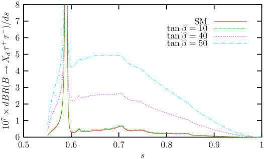
Figure 1: Differential branching ratio as a function of $s$, where $\xi=\pi/4$.

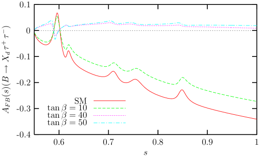
Figure 2: The forward-backward asymmetry as a function of $s$, where $\xi=\pi/4$.

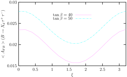
Figure 3: $<A_{FB}>$ as a function of $\xi$.

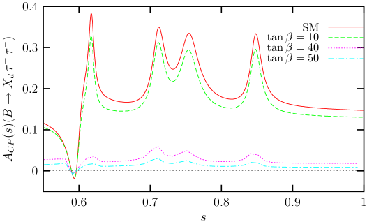
Figure 4: The CP asymmetry as a function of $s$, where $\xi=\pi/4$.

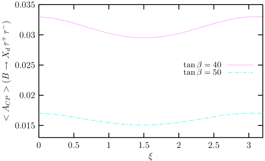
Figure 5: $<A_{CP}>$ as a function of $\xi$.

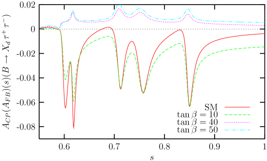
Figure 6: The CP asymmetry in the forward-backward asymmetry as a function of $s$, where $\xi=\pi/4$.

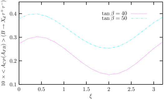
Figure 7: The CP asymmetry in the forward-backward asymmetry as a function of $\xi$.

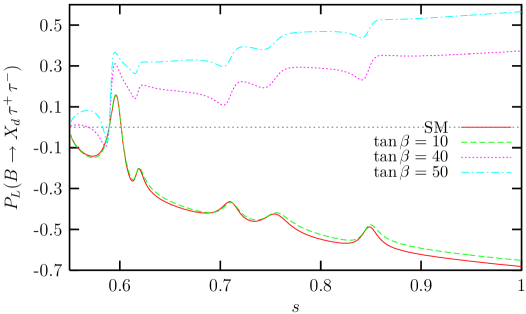
Figure 8: $P_{L}(s)$ as a function of $s$ , where $\xi=\pi/4$.

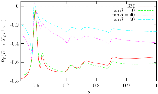
Figure 9: $P_{T}(s)$ as a function of $s$ , where $\xi=\pi/4$.

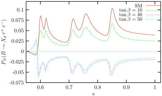
Figure 10: $P_{N}(s)$ as a function of $s$ , where $\xi=\pi/4$.

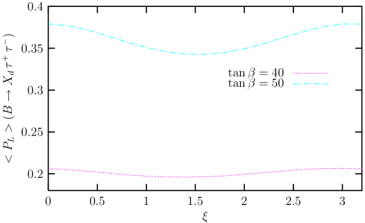
Figure 11: $<P_{L}>$ as a function of $\xi$.

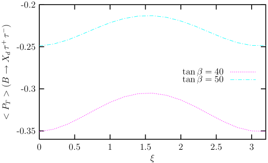
Figure 12: $<P_{T}>$ as a function of $\xi$.

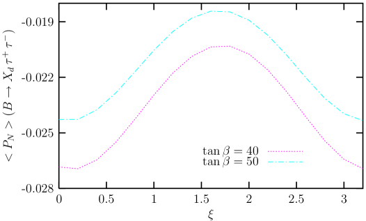
Figure 13: $<P_{N}>$ as a function of $\xi$. .