Running $G$ and $\Lambda$ at low energies from physics at $M_{X}$:
possible cosmological and astrophysical implications

Abstract:

The renormalization group (RG) approach to cosmology is an efficient method to study the possible evolution of the cosmological parameters from the point of view of quantum field theory (QFT) in curved space-time. In this work we continue our previous investigations of the RG method based on potential low-energy effects induced from physics at very high energy scales $M_{X}\lesssim M_{P}$. In the present instance we assume that both the Newton constant, $G$, and the cosmological term, $\Lambda$, can be functions of a scale parameter $\mu$. It turns out that $G(\mu)$ evolves according to a logarithmic law which may lead to asymptotic freedom of gravity, similar to the gauge coupling in QCD. At the same time $\Lambda(\mu)$ evolves quadratically with $\mu$. We study the consistency and cosmological consequences of these laws when $\mu\simeq H$. Furthermore, we propose to extend this method to the astrophysical domain after identifying the local RG scale at the galactic level. It turns out that Kepler’s third law of celestial mechanics receives quantum corrections that may help to explain the flat rotation curves of the galaxies without introducing the dark matter hypothesis. The origin of these effects (cosmological and astrophysical) could be linked, in our framework, to physics at $M_{X}\sim 10^{16-17}\,GeV$.

1 Introduction

The recent developments in physical cosmology have provided an astonishingly accurate picture of our universe, within the canons of the Friedmann-Lemaître-Robertson-Walker (FLRW) paradigm [1]. From these achievements emerged what has been called the cosmological concordance model, characterized by an essentially zero value of the spatial curvature parameter and a non-vanishing positive value of the cosmological constant (CC) term, $\Lambda$, in Einstein’s equations – or in general of some form of dark energy (DE) that cannot be attributed to any form of matter and radiation. This new standard cosmological model supersedes and refutes (by many standard deviations) the old Einstein-de Sitter (or critical-density) cosmological model, which has been the standard cosmological model until recently. The latter is also a spatially flat model, but it is characterized by a zero value of the cosmological constant. Evidence for the values of the cosmological parameters within the new concordance model comes both from tracing the rate of expansion of the universe with high-z Type Ia supernovae (SNe Ia) experiments [2, 3] and from the precise measurement of the anisotropies in the cosmic microwave background (CMB) radiation [4, 5]. These experiments indicate that the value of the cosmological constant is around

$$\Lambda_{0}=\Omega_{\Lambda}^{0}\,\rho_{c}^{0}\simeq 6\,h_{0}^{2}\times 10^{-47}\,GeV^{4}\,,$$ (1)

where $\Omega_{\Lambda}^{0}\sim 70\%$. Here $\rho_{c}^{0}\simeq\left(3.0\,\sqrt{h_{0}}\times 10^{-12}\,GeV\right)^{4}$ is the present value of the critical density and $H_{0}=100\,h_{0}$ km/s/Mpc, with $h_{0}=0.72\pm 0.08$, is the most precisely known value of Hubble’s constant [6]. In the context of the Standard Model (SM) of electroweak interactions, the physical (measured) value (1) should be the sum of the vacuum CC term in Einstein’s equations, $\Lambda_{vac}$, and the induced contribution from the vacuum expectation value of the Higgs effective potential, $\Lambda_{ind}=\langle V_{\rm eff}\rangle$, namely $\Lambda=\Lambda_{vac}+\Lambda_{ind}\,.$ Other contributions should be added within the SM, like those from QCD, but they are much smaller. It is only the combined parameter $\Lambda$ that makes physical sense, whereas both $\Lambda_{vac}$ and $\Lambda_{ind}$ remain individually unobservable– see e.g. [7] for a more detailed explanation. From the current LEP numerical bound on the Higgs boson mass, $\,M_{H}>114.4\,GeV$ (at the $95\%$ C.L.) [8], one finds $\,\,\,\left|\Lambda_{ind}\right|=(1/8)M_{H}^{2}\,v^{2}>1.0\times 10^{8}\,GeV^{4}$, where $v\simeq 246\,GeV$ is the vacuum expectation value of the Higgs field. Clearly, $\left|\Lambda_{ind}\right|$ is $55$ orders of magnitude larger than the observed CC value (1). Such discrepancy, the so-called “old” CC problem [9, 10], manifests itself in the necessity of enforcing an unnaturally exact fine tuning of the original cosmological term $\Lambda_{vac}$ in the vacuum action that has to cancel the induced counterpart $\,\Lambda_{ind}$ within a precision (in the SM) of one part in $\,10^{55}$. But the CC problem seems to be quite more general and it seems to plague all physical theories (QFT and string theory) making use of the concept of vacuum energy  [9, 10, 11]. Moreover, all attempts to deduce the small value of the cosmological constant from a sound theoretical idea involve some explicit or implicit form of severe fine-tuning among the parameters of the model. This became clear already from the first attempts to treat the dark energy component as a dynamical scalar field [12, 13, 14]. More recently this approach took the popular form of a “quintessence” field slow–rolling down its potential [15] and has adopted many different forms [16, 17]. The main motivation for the quintessence models is that they could provide a variable dark energy. Although there is no compelling reason for a time evolving DE at the moment – and it is difficult to get an experimental handle on it  [18]– it is even more difficult to accept (at least from the theoretical point of view) that the DE can be described by a static CC term in Einstein’s equations with the small value (1) throughout most of the history of the universe, namely after the electroweak phase transition took place.

An alternative possibility is to think of the DE as a time-evolving CC. This has been put forward from a purely phenomenological point of view in many places of the literature [19, 20]. However, a treatment of an evolving CC term from the more fundamental point of view of the renormalization group in QFT, with a direct link to Particle Physics, has been suggested only recently [21, 7, 22, 23]. The possible experimental consequences of this idea in the light of high-z SNe Ia data have also been tested in great detail in  [24] (see also the framework and analysis of [25, 26]). In the renormalization group method one takes the point of view that $\Lambda$ should not be constant, because the quantum effects may shift away the prescribed value, even if the latter is assumed to be zero [21]. In this approach the equation of state for the DE is the one for the “true” cosmological term $p_{\Lambda}=-\rho_{\Lambda}$. Hence it is fundamentally different from all kinds of quintessence-like proposals, where the CC is assumed to vanish precisely and the role of the DE is played by some new entity with a nontrivial equation of state. In the RG approach the CC becomes time-evolving, or redshift dependent: $\Lambda=\Lambda(z)$. Although we do not have a quantum theory of gravity where the running of the gravitational and cosmological constants could ultimately be substantiated, a semiclassical description within the well established formalism of QFT in curved space-time (see e.g. [27, 28]) should be a good starting point. From the RG point of view, $\Lambda$ becomes a scaling parameter $\Lambda(\mu)$ whose value should be sensitive to the entire energy history of the universe – in a manner not essentially different to, say, the electromagnetic coupling constant in QED or the gauge coupling constant in QCD.

While the RG method to tackle the CC problem has been used earlier [29, 30, 31], the decoupling effects of the massive particles at low energies may change significantly the structure of the renormalization group equations (RGE) with important phenomenological consequences. This feature has been pointed out recently by several authors from various interesting points of view [22, 7]. However, it is not easy to achieve a RG cosmological model where $\Lambda$ runs smoothly without fine tuning at the present epoch. In Ref.  [23, 32] a successful attempt in this direction has been made, which is based on possible quantum effects near a high mass scale $M_{X}$, not far away from the Planck scale $M_{P}$, that are transferred (via soft decoupling) to the low energy physics. At the same time, the approximate coincidence of the observed CC and the matter density, $\ \Omega_{\Lambda}^{0}\sim\Omega_{M}^{0}\,$ (i.e. the “new” CC problem, or “time coincidence problem” [9, 10]) can be alleviated in this framework [32]. Thus the RG cosmologies constitute a healthy alternative to the ad hoc quintessence models and are worth exploring. In the present paper we generalize the RG approach developed in [7, 22, 23, 32] by including the possibility to have a running Newton’s constant as well . A fundamental question that we address here is the possibility to maintain the phenomenologically successful quadratic evolution law $\delta\Lambda\sim H^{2}$ (emerging from an RGE of the form $d\Lambda/d\ln H\propto H^{2}$) as proposed in [7, 23, 32], also in a $G$-running framework. This law is based on the assumption that the physical RG scale is defined by $\mu=H$, the Hubble parameter. We will see that this Ansatz is consistent with the systematic RG scale-setting procedure proposed recently in [36]. In addition, the $\delta\Lambda\sim H^{2}$ law is the only one among those that are consistent with this procedure which could have measurable phenomenological consequences. Therefore, it is of foremost importance to explore its phenomenological viability, in spite of the insurmountable technical difficulties encountered at present for an explicit calculation in QFT on a curved background [37]. In this sense it is remarkable that the quadratic law $\delta\Lambda\sim H^{2}$ can also be motivated from very general arguments in QFT [38] which may go beyond the RG. No less appealing is that this quadratic law can further be claimed, at least heuristically, on the grounds of the so-called Holographic Principle (HP) applied to effective field theories [39]. In fact, by linking IR and UV scales through entropy bounds, the HP may provide essential ingredients to relate the microscopic world of Particle Physics and the large scale structure of the Universe . A main result of this paper is that the adoption of that quadratic law will lead us to an alternative cosmological RG framework to that presented in Ref. [23, 32], keeping though all the nice phenomenological features of the latter, however with the distinctive property of having a (logarithmically) running gravitational constant. This last property endows the new cosmological model with potentially far-reaching phenomenological implications both at the cosmological and astrophysical level which will be explored in some detail in this paper.

The structure of the paper is as follows. In the next section we introduce a few general features of the cosmological models based on variable $G$ and $\Lambda$. In Section 3 we provide some general discussion of the RG cosmological models. The consistency of the RG scale setting in cosmology is discussed in Section 4. In Section 5 we focus on the cosmological model presented here, characterized by a logarithmic running of $G$ and a quadratic running of $\Lambda$. The numerical analysis of this model is presented in Section 6, where we also show the predicted deviations from the standard FLRW expectations. In Section 7 we narrow down the applicability of this RG cosmological model to the astrophysical domain by considering the possibility to attribute the origin of the flat rotation curves of the galaxies to a RG quantum correction to Kepler’s third law of celestial mechanics. We close with some final discussion in the last section, where we draw our conclusions.

2 Variable $G$ and $\Lambda$ cosmologies

The cosmological constant contribution to the curvature of space-time is represented by the $\lambda\,g_{\mu\nu}$ term on the l.h.s. of Einstein’s equations. The latter can be absorbed on the r.h.s. of these equations

$$R_{\mu\nu}-\frac{1}{2}g_{\mu\nu}R=8\pi G\ \tilde{T}_{\mu\nu}\,,$$ (2)

where the modified $\tilde{T}_{\mu\nu}$ is given by $\tilde{T}_{\mu\nu}\equiv T_{\mu\nu}+g_{\mu\nu}\,\Lambda$. Here $T_{\mu\nu}$ is the ordinary energy-momentum tensor associated to isotropic matter and radiation, and the new CC term $\Lambda=\lambda/8\pi\,G\equiv\rho_{\Lambda}$ represents the vacuum energy density. Modeling the expanding universe as a perfect fluid with velocity $4$-vector field $U^{\mu}$, we have

$$T_{\mu\nu}=-p\,g_{\mu\nu}+(\rho+p)U_{\mu}U_{\nu}\,,$$ (3)

where $p$ is the proper isotropic pressure and $\rho$ is the proper energy density of matter-radiation. Clearly the modified $\tilde{T}_{\mu\nu}$ defined above takes the same form as (3) with $\rho\rightarrow\tilde{\rho}=\rho+\Lambda$ and $\ p\rightarrow\tilde{p}=p-\Lambda$. With this generalized energy-momentum tensor, and in the FLRW metric ($k=0$ for flat, $k=\pm 1$ for spatially curved, universes)

$$ds^{2}=dt^{2}-a^{2}(t)\left(\frac{dr^{2}}{1-k\,r^{2}}+r^{2}\,d\theta^{2}+r^{2}\,\sin^{2}\theta\,d\phi^{2}\right)\,,$$ (4)

the gravitational field equations boil down to Friedmann’s equation

$$H^{2}\equiv\left(\frac{\dot{a}}{a}\right)^{2}=\frac{8\pi\,G}{3}\tilde{\rho}-\frac{k}{a^{2}}=\frac{8\pi\,G}{3}\left(\rho+\Lambda\right)-\frac{k}{a^{2}}\,,$$ (5)

and the dynamical field equation for the scale factor:

$$\ddot{a}=-\frac{4\pi}{3}G\,(\tilde{\rho}+3\,\tilde{p})\,a=-\frac{4\pi}{3}G\,(\rho+3\,p-2\,\Lambda)\,a\,.$$ (6)

The measured CC is the parameter $\Lambda$ entering equations (5) and (6), which are used to fit the cosmological data [2, 3]. Let us next contemplate the possibility that $G=G(t)$ and $\Lambda=\Lambda(t)$ can be both functions of the cosmic time. This is allowed by the Cosmological Principle embodied in the FLRW metric (4). Then the Bianchi identities imply that $\bigtriangledown^{\mu}\,\left({G\,\tilde{T}}_{\mu\nu}\right)=0$, and with the help of the FLRW metric a straightforward calculation yields

$$\frac{d}{dt}\,\left[G(\Lambda+\rho)\right]+3\,G\,H\,(\rho+p)=0\,.$$ (7)

This equation just reflects the purely geometric Bianchi identity satisfied by the tensor on the l.h.s. of Einstein’s equations (2) in terms of the physical quantities (energy densities, pressure and gravitational coupling) on its r.h.s. It is easy to check that (7) constitutes a first integral of the dynamical system (5) and (6). However, this general constraint on the physical quantities is too complicated in practice, and it is difficult to understand it on physical grounds because it does not generally lead to a local energy-momentum conservation law. Let us consider some simpler cases. The simplest possible case is when both $G$ and $\Lambda$ are constant. When $G$ is constant, the identity above implies that $\Lambda$ is also a constant, if and only if the ordinary energy-momentum tensor is individually conserved ($\bigtriangledown^{\mu}\,{T}_{\mu\nu}=0$), i.e.

$$\dot{\rho}+3\,H\,(\rho+p)=0\,.$$ (8)

However, a first non-trivial situation appears when $\Lambda=\Lambda(t)$ but $G$ is still constant. Then a first integral of the system (5) and (6) is given by

$$\dot{\Lambda}+\dot{\rho}+3\,H\,(\rho+p)=0\,.$$ (9)

This result is simpler than (7), and has the advantage that it can still be interpreted as a physical conservation law. The conserved (total) energy density here is the sum of the matter-radiation energy density, $\rho=\rho_{M}+\rho_{R}$, plus the dark energy density embodied in $\rho_{\Lambda}\equiv\Lambda$. Of course $\rho_{M}$ includes the contribution from the purported cold dark matter (CDM), which should be dominant. Alternatively, using the metric (4) one may derive (9) directly from $\bigtriangledown^{\mu}\,{\tilde{T}}_{\mu\nu}=0$, as this is obviously a particular case of (7). This possibility shows that a time-variable CC cosmology may exist such that transfer of energy occurs from matter-radiation into vacuum energy, and vice versa. From the point of view of general covariance there is no problem because the latter is tied to the conservation of the full energy-momentum tensor, which in this case is $\tilde{T}_{\mu\nu}$ rather than ${T}_{\mu\nu}$. We remark that while the decay of the vacuum energy into ordinary matter and radiation could be problematic for the observed CMB, the decay into CDM could be fine [16, 41]. The detailed analysis of a time-variable CC cosmology in the light of high-z SNe Ia data carried out in Ref. [24] was precisely based on this framework.

In this paper we make a step forward by entertaining the possibility that $G$ can also be a function of the cosmic time, $G=G(t)$, together with $\Lambda=\Lambda(t)$. Although we have seen that the most general case should fulfill the general constraint (7), we still want to keep the usual matter-radiation conservation law (8) as this represents the canonical (i.e. the simplest) cosmological model with variable $G$ and $\Lambda$ possessing a physical conservation law. In this model there is no transfer of energy between matter-radiation and dark energy. However, the time evolution of $\Lambda$ is still possible at the expense of a time varying gravitational constant. Indeed, it is easy to see that in this case the following (hereafter called canonical) differential constraint must be satisfied:

$$(\rho+\Lambda)\,\dot{G}+G\,\dot{\Lambda}=0\,.$$ (10)

Again this is a particular case of (7). The solution of a generic cosmological model of this kind with variable $G$ and $\Lambda$ is contained in part in the coupled system of differential equations (5), (8) and (10), together with the equation of state $p=p(\rho)$ for matter and radiation. However, still another equation is needed to completely solve this cosmological model in terms of the fundamental set of variables $(H(t),\rho(t),p(t),G(t),\Lambda(t))$. Many relations have been proposed in the literature from the purely phenomenological point of view [19, 20]. In the next section we discuss the possibility that the fifth missing equation is a relation of the form $\Lambda=\Lambda(H)$. Most important, we will motivate this relation at a fundamental QFT level, specifically within the context of the renormalization group in curved space-time, and then discuss the possible form of the associated RG evolution law for the gravitational constant.

3 Renormalization group cosmologies

Following the approach of [7, 22, 23, 32] we describe the scaling evolution of $\Lambda$ by introducing a renormalization group equation for the cosmological constant. The connection between scaling evolution and time evolution is to be made in a second step. From dimensional analysis, and also from dynamical features discussed in the aforementioned references, the RGE may take in principle the generic form

$$\frac{d\Lambda}{d\ln\mu}=\sum_{n}\,A_{n}\,\mu^{2n}\,.$$ (11)

Here $\mu$ is the energy scale associated to the RG running. Furthermore, in a RG cosmology with a time-evolving $G$ we expect a RGE for $G$ as well. This is best formulated in terms of $G^{-1}$ as follows:

$$\frac{d}{d\ln\mu}\left(\frac{1}{G}\right)=\sum_{n}\,B_{n}\,\mu^{2n}\,.$$ (12)

It will prove convenient for further reference to introduce the integrated form of these equations:

$$\Lambda(\mu)=\sum_{n}\,C_{n}\,\mu^{2n}\,,\ \ \ \ \ \ \frac{1}{G(\mu)}=\sum_{n}\,D_{n}\,\mu^{2n}\,.$$ (13)

Coefficients $A_{n},B_{n},C_{n}$ and $D_{n}$ in these formulas are obtained from a sum of the contributions of fields of different masses $M_{i}$. The r.h.s. of (11) and (12) define the $\beta$-functions for $\Lambda$ and $G^{-1}$ respectively, which are functions of the masses and in general also of the ratios between the RG scale $\mu$ and the masses. For $\mu\ll M_{i}$, the series above are in principle assumed to be expansions in powers of the small quantities $\mu/M_{i}$ [7, 22]. However, the possibility to extend the analytical properties of some of these expansions will be discussed later. We assume that $\mu$ is of the order of some physical energy-momentum scale characteristic of the FLRW cosmological setting, and can in principle be specified in different ways. In the $\Lambda$-running framework of [7], it was assumed that $\mu$ is given by the typical energy-momentum of the cosmological gravitons of the background FLRW metric. This suggests we can set $\mu\simeq H$ (Hubble parameter), which is of the order of the square root of the curvature scalar in the FLRW metric, $\mu\sim R^{1/2}$.

In the cosmological applications, e.g. when considering the evolution of the present universe, we are going to keep the Ansatz $\mu\simeq H$. We will claim that it is a sound RG scale-setting also for a framework based on running $\Lambda$ and $G$. The consistency of this choice will be discussed in Section 4 in the light of the scale-setting procedure devised in [36]. For the moment we observe that, within the $\mu\simeq H$ Ansatz, the RGE (11) above defines a relation of the type $\Lambda=\Lambda(H)$, and therefore provides the fifth equation suggested at the end of the previous section, needed to solve the cosmological model. At the same time Eq. (12) defines a relation of the sort $G=G(H)$. Obviously these two functions of $H$ cannot be independent, for the Bianchi identity imposes the differential constraint (10) in which $\rho=\rho(t)$ is a known function obtained after solving (8) – once the equation of state $p=p(\rho)$ for matter and radiation is specified. Put another way: consistency requires that the two expansions (11) and (12) ought to be interconnected via the differential constraint (10), so that if one of the expansions is given the other can be retrieved from the Bianchi identity. For example, in Ref. [23] we suggested the following specific form for the RGE (11)

$$\frac{d\Lambda}{d{\ln\mu}}=\frac{1}{(4\pi)^{2}}\ \sigma\,\mu^{2}M^{2}+...\,,$$ (14)

with $\mu=H$. Here we have defined the effective mass parameter

$$M\equiv\left|\sum_{i}\,c_{i}\,M_{i}^{2}\right|^{1/2}\,,$$ (15)

and $\,\sigma=\pm 1$ indicates the sign of the overall $\beta_{\Lambda}$-function, depending on whether the fermions ($\sigma=-1$) or bosons ($\sigma=+1$) dominate at the highest energies. The form (14) for the RGE is based on the leading participation of the heaviest possible masses $M_{i}$ in the expansion. These masses could arise e.g. from some Grand Unified Theory (GUT) whose energy scale $M_{X}$ is just a few orders of magnitude below $M_{P}$. The form (14) results from truncating the series (11) at $n=1$. The term $n=0$, corresponding to contributions proportional to $M_{i}^{4}$, must be absent if we want to describe a successful phenomenology [23, 24]. Actually, from the RG point of view it is forbidden because in the physics of the modern Universe we probe a range of energies where $\mu$ is always below the superheavy masses $M_{i}$. In addition, dimensional analysis and dynamical expectations tell us that the remaining terms are suppressed by higher powers of $\mu/M_{i}$  [7, 22, 23]. In the absence of experimental information, the numerical choice of $\,\sigma\,M^{2}\,$ is model-dependent. For example, the fermion and boson contributions in (11) might cancel due to supersymmetry (SUSY) and the total $\beta$-function becomes non-zero at lower energies due to SUSY breaking. Another option is to suppose some kind of string transition into QFT at the Planck scale. Then the heaviest particles would have masses comparable to the Planck mass $M_{P}$ and represent the remnants, e.g., of the massive modes of a superstring.

The obvious motivation for this RG scenario [23, 32] is that the r.h.s. of (14) is of the order of the present value of the CC. To assess this in more detail, let us integrate Eq. (14) straightforwardly. We find an evolution law for $\Lambda$ which is quadratic in $\mu$  and can be expressed, with the help of the notation (13), as follows:

$$\Lambda(\mu)=C_{0}+C_{1}\,\mu^{2}\,,\\$$ (16)

where

$$C_{0}=\Lambda_{0}-\frac{3\,\nu}{8\pi}M_{P}^{2}\,\mu_{0}^{2}\,,\ \ \ C_{1}=\frac{3\,\nu}{8\pi}\,M_{P}^{2}\,.$$ (17)

Within our Ansatz for the RG scale, $\mu_{0}$ stands for the present day value of the Hubble parameter, $H_{0}$, and the coefficient $\nu$ is essentially the ratio between the squares of the effective GUT mass scale $M$ and the Planck scale up to $\sigma=\pm 1$, depending on whether bosonic or fermionic fields dominate in the mass spectrum below the Planck scale:

$$\nu=\frac{\sigma}{12\pi}\frac{M^{2}}{M_{P}^{2}}\,.$$ (18)

This parameter was first defined in Ref. [23, 24]. Irrespective of the precise meaning of $\nu$ in the context of QFT in curved space-time, the latter reference suggested also how to use $\nu$ to parametrize deviations of the evolution laws from the standard FLRW cosmology . Equation (16) is normalized such that $\Lambda$ takes its present day value $\Lambda_{0}$ for $\mu=\mu_{0}$. The highest possible value of the heavy masses $M_{i}$ is $M_{P}$, and therefore we typically expect that the effective mass (15) is of the same order. However, due to the multiplicities of the heavy masses, we cannot exclude a priori that $M>M_{P}$. To be conservative we will take

$$|\nu|=\nu_{0}\equiv\frac{1}{12\pi}\simeq 0.026$$ (19)

as the typical value of $\nu$, corresponding to $M=M_{P}$. A very nice feature of this RG picture for $\Lambda$ is that its evolution, being smooth and sufficiently slow in the present Universe, may still encapsulate non-negligible effects that could perhaps be measured . In fact, the predicted rate of change of $\Lambda$ (in other words, the value of its $\beta$-function) at $\mu=H_{0}$ is of order of $\Lambda_{0}$ itself:

$$\beta_{\Lambda}^{0}\sim C_{1}\,H^{2}\left|{}_{t=t_{0}}\right.=\frac{3\,\nu}{8\pi}\,M_{P}^{2}\,H_{0}^{2}\lesssim 10^{-47}\,GeV^{4}\,.$$ (20)

In contrast, at the earliest times when $H\simeq M_{P}$, the same RGE predicts a CC of order $\Lambda\sim M_{P}^{4}$, which again is a natural expectation. If we define the energy scale $E_{\Lambda}(t)\equiv\Lambda(t)^{1/4}$ associated to the vacuum energy density $\rho_{\Lambda}\equiv\Lambda$ at any given moment of the history of the Universe, the RGE above may explain [23, 32] why the millielectronvolt energy associated to the present value $\Lambda_{0}$ happens to be the geometrical mean of the two most extreme energy scales in our Universe, $H_{0}\sim 10^{-42}\,GeV$ (the value of $\mu$ at present) and $M_{P}\sim 10^{19}\,GeV$:

$$E_{\Lambda}(t=t_{0})\equiv\Lambda_{0}^{1/4}\simeq\sqrt{M_{P}\,H_{0}}={\cal O}\left(10^{-3}\right)\,eV\,.$$ (21)

Amusingly this is also the order of magnitude of another, independent, cosmic energy scale: the one associated to matter density, $E_{M}(t)\equiv\rho_{M}^{1/4}(t)$. Assuming $k=0$ and $\Lambda=0$ in Friedmann’s equation (5), the energy scale associated to the matter density at present is seen to be $E_{M}(t_{0})\sim\sqrt{M_{P}\,H_{0}}$. Remarkably the dark energy scale (21) associated to our RG cosmological framework coincides with the matter density scale defined by Friedmann’s equation at $t=t_{0}$, and therefore it helps to explain the so-called “coincidence problem” [10], one of the two fundamental conundrums behind the cosmological constant problem.

A value of $\nu$ of order of $10^{-2}-10^{-3}$ suggests that there might be some physics just 2 orders of magnitude below the Planck scale, i.e. around $10^{17}\,GeV$. This would be indeed the mass scale of the heavy masses $M_{i}$ if we assume some multiplicity of order $100$ in the number of the heaviest degrees of freedom in a typical GUT. To see this, rewrite (18) with $\nu=10^{-3}$ as

$$\sum_{i}c_{i}\,M_{i}^{2}=12\,\pi\,M_{P}^{2}\,\nu=12\,\pi\,(1.2\times 10^{19}\,GeV)^{2}\,10^{-3}\simeq 5.4\times 10^{36}\,GeV^{2}\,.$$ (22)

Then if we assume $M_{i}=M_{X}$, $c_{i}\sim 1$ for all $i$, it follows that

$$M_{X}\sim 10^{17}\,GeV\ \ \ {\rm for}\ \ \ \sum_{i}\,c_{i}\sim 100\,.$$ (23)

Therefore, there is the possibility that the origin of this RG cosmology could bare some relation to physics near the SUSY-GUT scale.

From the previous considerations we realize that the models based on the RG evolution of $\Lambda$ could be serious competitors to e.g. quintessence models (and generalizations thereof) to account for some of the fundamental issues behind the multifarious cosmological constant problem [9, 10], and moreover they are also testable in the next generation of high-z SNe Ia experiments (such as SNAP[43]) – as has been demonstrated in great detail in  [24]. The RG cosmological model analyzed in the last reference, although it constitutes a running $\Lambda$ model, is a fixed-$G$ model. In contrast, the RG model under consideration aims at preserving the virtues of the quadratic law (16) for the $\Lambda$ evolution (i.e. the rich phenomenology potential unraveled in  [24]) while allowing for a simultaneous evolution of the gravitational constant, $G$. This may add distinctive features and new phenomenological tests to be performed. Obviously it is important to analyze this possibility in order to distinguish between these two RG cosmological models and also to fully display the power of the RG approach versus the other dark energy models [10].

4 On the RG scale-setting procedure in cosmology

In this section we consider the consistency of the RG scale choice in certain problems related to the cosmological framework. Specifically, we discuss the consistency of our choice $\mu\simeq H$ for the application to the large scale cosmological problems along the lines of the procedure recently proposed in [36]. In the next two sections we shall concentrate on the construction of a cosmological model based on the RG approach, and only in the last part of our work we will try to extend these methods to the local (galactic) domain. Let us commence with the scale setting at the cosmological level. Starting from the canonical constraint (10) we trade the cosmic time for a generic scale parameter $\mu$ (without specifying its relation to physics at this point), and rewrite it in the following way [36]:

$$\left[(\rho+\Lambda(\mu))\,\frac{dG(\mu)}{d\mu}+G(\mu)\,\frac{d\Lambda(\mu)}{d\mu}\right]\,\frac{d\mu}{dt}=0\,.$$ (24)

Obviously, the matter-radiation energy density $\rho$ is the only parameter which can not be defined as a function of $\mu$ directly because it is unrelated to the RG in the first place. However, since $G$ and $\Lambda$ are primarily functions of $\mu$ in the RG framework, the differential constraint (24) can be used to eventually define $\rho$ as a function of $\mu$ . If $d\mu/dt\neq 0$, it is easy to check that we can isolate $\rho$ as follows:

$$\rho=-\Lambda(\mu)+\frac{1}{G(\mu)}\,\frac{d\Lambda(\mu)}{d\mu}\left(\frac{d}{d\mu}\,\frac{1}{G(\mu)}\right)^{-1}\,.$$ (25)

This scale-setting algorithm defines a relation $\rho=f(\mu)$ between the cosmological data, represented by $\rho$, and the scaling functions of $\mu$. Under appropriate conditions, this relation can be inverted to find $\mu$ as a function of the external data: $\mu=f^{-1}(\rho)$. Since this function has been determined by the Bianchi identity, it should define a valid set of RG scales for cosmology. In other words, the specific scale $\mu$ to be used in cosmology should be chosen among the class of (potentially multivalued) functions obtained by this procedure under the condition that the scale so obtained is positive-definite and is a smooth function of the cosmological parameters. Further (physical) criteria may be needed to ultimately select one particular function within this class.

Assuming that this is a valid method to define the RG scale, we are now in position to develop a scenario with simultaneous running of the parameters $G$ and $\Lambda$ in which the choice $\mu\simeq H$ is compatible with the aforementioned scale-setting procedure. To realize this scenario we stick to our RGE for $\Lambda$ as given in (14) – hence to the quadratic running law (16) – and we seek for a suitable RGE for $G^{-1}$. It cannot be an independent equation once the RGE for $\Lambda$ has been established. Therefore, this restriction provides a method to hint at possible forms for the RGE (12) compatible with the canonical constraint (10). For example we could start with an expansion akin to that in Eq. (3.1) of  [24] for $\Lambda$:

$$(4\pi)^{2}\,\frac{d}{d\ln\mu^{2}}\left(\frac{1}{G}\right)=\sum_{i}\,a^{\prime}_{i}\,M_{i}^{2}+\sum_{i}\,b^{\prime}_{i}\,M_{i}^{2}\left(\frac{\mu}{M_{i}}\right)^{2}+\sum_{i}\,c^{\prime}_{i}\,M_{i}^{2}\left(\frac{\mu}{M_{i}}\right)^{4}+...$$ (26)

Since the cosmological RG scale $\mu$ is assumed to be very small for the present universe, and the series is supposed to be convergent, we expect that the first term in this expansion is the crucial one and the remaining terms are inessential. Indeed, selecting the first term we are led to a RGE of the type

$$\frac{d}{d\ln\mu^{2}}\left(\frac{1}{G}\right)=\,\nu\,M_{P}^{2}+...\,.$$ (27)

Consider now the generic expansions (11)-(13) for $\Lambda$ and $G^{-1}$. In particular notice the following relations among the coefficients for $n=0$:

$$C_{0}=\Lambda_{0}+A_{0}\,\ln\frac{\mu}{\mu_{0}}-\frac{1}{2}\,A_{1}\,\mu_{0}^{2}-\frac{1}{4}\,A_{2}\,\mu_{0}^{4}+...$$

$$D_{0}=M_{P}^{2}+B_{0}\,\ln\frac{\mu}{\mu_{0}}-\frac{1}{2}\,B_{1}\,\mu_{0}^{2}-\frac{1}{4}\,B_{2}\,\mu_{0}^{4}+...\,,$$ (28)

where $\mu_{0}$ is the normalization point corresponding to the $t=t_{0}$ moment of time. The coefficients (4) play a role in computing explicitly the r.h.s. of (25). In particular notice that $A_{0}=0$, to be consistent with (17)(cf. Ref. [23]). Also important is that the scale derivative of $D_{0}$ is non-vanishing,

$$D_{0}^{\prime}\equiv\frac{dD_{0}}{d\mu}=\frac{B_{0}}{\mu}=\frac{\sigma}{6\pi}\,\frac{M^{2}}{\mu}\,.$$ (29)

Here we have used $B_{0}=2\,\nu\,M_{P}^{2}=\sigma\,M^{2}/6\,\pi$ as seen from (27) and (18). This result shows that $G^{-1}$ is actually non-analytic at $\mu=0$, a fact to which we shall return later. With these relations in mind, a straightforward calculation of the r.h.s. of Eq (25), using the expansions (13), leads to

$$\rho\simeq-C_{0}+C_{1}\left(\frac{2\,D_{0}}{B_{0}}-1\right)\,\mu^{2}+...$$ (30)

where we have neglected the higher order terms in $\mu$. Next we substitute the coefficients (17) in (30) and use the fact that $D_{0}\simeq M_{P}^{2}$. Irrespective of the sign $\sigma=\pm 1$, the resulting equation determining $\mu$ is amazingly simple:

$$\mu^{2}\simeq\frac{\rho+C_{0}}{C_{1}\left(\frac{2\,M_{P}^{2}}{B_{0}}-1\right)}\simeq\frac{8\pi}{3}\,\frac{\rho+\Lambda_{0}}{M_{P}^{2}}=H^{2}\,,$$ (31)

where the last equality makes use of Friedmann’s equation (5) in the flat case. Our starting Ansatz $\mu=H$ is, therefore, explicitly borne out within the criterion defined by Eq. (25)  (q.e.d.).

The previous proof relies on the expansions (11)-(13) advocated in the literature [7, 22, 23, 36]. Notwithstanding, this does not exhaust the list of possibilities made available to us by the Bianchi identity in the canonical form (10). It is still possible to extract the same phenomenology if we make allowance for an extended RGE for $G$ beyond an expansion in (integer) powers of the small parameters $\mu/M_{i}$. Then other (non-analytic) contributions may arise. We shall discuss this possibility along the second part of the next section.

5 A cosmological model with logarithmic running of G and quadratic running of $\Lambda$

In the previous section we have established a scenario where the choice $\mu\simeq H$ is a consistent scale setting for cosmological considerations. Let us use this RG framework and apply it to a spatially flat Universe, i.e. $k=0$ in Eq. (5). This situation is not only the simplest one, but it corresponds (as already mentioned in the introduction) to the preferred scenario in the light of the present data from distant supernovae and the CMB. Moreover, the $k=0$ Universe already captures all the main traits of the new RG cosmology with variable $G$ without introducing additional complications related to curvature. By collecting Friedmann’s equation, the quadratic RG evolution law for $\Lambda$, and the (canonical) differential constraint imposed on the functions $G(t)$ and $\Lambda(t)$ by the Bianchi identity, we can set up the system:

$$\rho+\Lambda=\frac{3H^{2}}{8\,\pi\,G}\,,$$

$$\Lambda=C_{0}+C_{1}\,H^{2}\,,$$ (32)

$$(\rho+\Lambda)\,d{G}+G\,d{\Lambda}=0\,.$$

This system can be immediately solved for the function $G=G(H;\nu)$ depending of the parameter $\nu$, with the result

$$G(H;\nu)=\frac{G_{0}}{1+\nu\,\ln\left(H^{2}/H_{0}^{2}\right)}\,,$$ (33)

where $G(H_{0})=G_{0}\equiv 1/M_{P}^{2}$. In this way we have obtained explicitly the corresponding running law for $G$ as a function of the RG scale $\mu=H$. From this law we learn that for $\nu>0$ the gravitational constant $G$ decreases logarithmically with $H$, hence very slowly, which is an extremely welcome feature in view of the experimental restrictions on $G$ variation (see later on). Such a decreasing behavior with the cosmological energy scale $\mu=H$ is equivalent to say that the law that we have obtained nicely corresponds to an asymptotically free regime for $\nu>0$, much in the same way as the strong coupling constant in QCD. In addition, we discover that the parameter $\nu$ defined in (18) plays essentially the role of the (dimensionless) $\beta$-function for $G$. Finally, we note that the function (33) is non-analytic, which was expected from a remark made in Section 4.

Consistency with the Bianchi identity requires that Eq. (33) must be the solution of the RGE (12) for $G^{-1}$. To check this, we note that in leading order the last equation boils down to Eq. (27). Integrating this equation under the boundary condition $G(\mu=\mu_{0})=G_{0}$ we immediately recover Eq. (33), as desired. Had we ignored the first term in (26) and assumed that the first leading contribution comes from the second term (i.e. the one proportional to $\mu^{2}=H^{2}$) we would have obtained

$$G(H)=\frac{G_{0}}{1+\zeta\,G_{0}\,(H^{2}-H^{2}_{0})}\,,$$ (34)

instead of (33), where $\zeta$ is a dimensionless coefficient. The resulting scenario is not very appealing as it does not lead to any phenomenological consequence to speak of. In fact, if we substitute (34) in (10) and integrate the resulting equation, the following evolution law for the CC ensues:

$$\Lambda(H)=\Lambda_{0}+\frac{3\,\zeta}{16\pi}\,(H^{4}-H_{0}^{4})\,.$$ (35)

Although this quartic law is – as the quadratic one (16)– smooth and mathematically possible, it leads to absolutely no phenomenology due to the smallness of the Hubble parameter at the present time: $H_{0}\sim 10^{-42}\,GeV$. Similarly, the square dependence $G_{0}\,H^{2}=H^{2}/M_{P}^{2}$ in the running law for $G$ given by (34) is extremely weak. Therefore, it is clear that only if the first term of the r.h.s. of (26) is non-vanishing it is possible to meet the logarithmic law (33) for $G$ and the quadratic law (16) for $\Lambda$. This combination of RG laws is the only one compatible with the canonical constraint (10) that may lead to a cosmological model with a rich phenomenology comparable to the model presented in [23, 24].

A remark is now in order. As the reader could readily notice, by admitting that the first term of the r.h.s. of (26) is non-vanishing, we are departing from the decoupling theorem [45] and assume the non-standard form of decoupling for the parameter $1/G$. In order to justify this departure from the canonical form of decoupling, let us remember that the attempt to derive the gravitational version of the decoupling theorem [37] was successful only in that sector of the gravitational action which is available in the linearized gravity framework. In the cases of $\Lambda$ and $1/G$ the explicit derivation of the decoupling law requires a new technique of calculation which should take the non-trivial and dynamical nature of the metric background into account. In the actual phenomenological approach it is primarily the Bianchi identity (rather than the decoupling theorem) that decides about the evolution of $G$ once the evolution of $\Lambda$ has been ordered. In this sense, the final structure for the RGE of $G$ can be of the form (14) even if this does not fulfill the standard expectations from the decoupling theorem. This uneven status between the two parameters can be understood on physical grounds, in the sense that the ultimate origin of $G$ and $\Lambda$ and their role in defining the background geometry may be essentially different. $\Lambda$ can be viewed as a small parameter in QFT: this can be technically implemented by allowing for a fine-tuning of the renormalization condition for the vacuum counterpart of the cosmological term – see the Introduction. At the same time the situation with $1/G$ is quite different. For example, it could be that the Planck mass is not only some threshold scale for the quantum gravity effects but, after all, a real mass. One can imagine that the non-perturbative phenomena of quantum gravity are involved to generate this scale and then the standard decoupling law (which is essentially a perturbative result) would not apply to the parameter $1/G$.

We shall finish this section by presenting additional arguments concerning our choice for the identification of the scale parameter $\mu$ with the Hubble parameter $H$ at low energies. These arguments do not look superfluous in view of the distinct choices for $\mu$ which one can meet in the existing literature [21, 7, 22, 23, 25, 36]. If one allows for some generalization of the expansions (13), it may have an impact on the scale setting. It is thus advisable not to assume a priori the result $\mu=H$ derived in (31), although we want to show that under certain conditions we can also retrieve a similar scale setting. On physical grounds we cannot exclude a priori the presence of non-perturbative and/or non-local effects in the far IR [44]. Whereas at higher energies the behavior of $G(\mu)^{-1}$ is influenced by the higher powers of $\mu$ in (13), the running in the present day Universe is controlled by the first coefficient $B_{0}$ in (12), which in turn leads to a non-analytical behavior of $D_{0}=D_{0}(\mu)$ as a function of $\mu$ in the series (13). In other words, at the present IR energies the expansion $G^{-1}$ in powers of $\mu$ may not be a pure Taylor expansion. Baring in mind these considerations, let us generalize the picture as follows. Assume that in the far IR the expansions (13) take contributions of the form

$$\Lambda(\mu)=a_{0}+a_{1}\left(\frac{\mu}{\mu_{0}}\right)^{\alpha}\,,\ \ \ \frac{1}{G(\mu)}=b_{0}+b_{1}\left(\frac{\mu}{\mu_{0}}\right)^{\beta}\,,$$ (36)

where we assume arbitrary coefficients $a_{0},b_{0},a_{1},b_{1}$ and arbitrary exponents $\alpha,\beta$, which can be smaller than one. From these general expressions we may compute the corresponding RG scale following from (25). At the end of the calculation we encounter the result:

$$\rho+a_{0}=\frac{a_{1}}{\beta}\left[(\alpha-\beta)\left(\frac{\mu}{\mu_{0}}\right)^{\alpha}+\alpha\,\,\frac{b_{0}}{b_{1}}\,\left(\frac{\mu}{\mu_{0}}\right)^{\alpha-\beta}\right]\,.$$ (37)

This example already shows that even in relatively simple situations it may be difficult to find the explicit relation $\mu=f^{-1}(\rho)$ mentioned in Section 4. It also shows that the scale setting $\mu\simeq H$ will not always be possible. And, most important, it also helps us to find situations when it is actually possible. Indeed, let us consider a generic case where the RGE for $G^{-1}$ takes terms of the form

$$\frac{d}{d\ln\mu^{2}}\ \left(\frac{1}{G}\right)=\nu\,M_{P}^{2}\,\left(\frac{\mu^{2}}{M^{2}}\right)^{\gamma}\,.$$ (38)

For any $\gamma>0$ (integer or not) this expression does respect the decoupling theorem, in contrast to (26). By integrating (38) we are led to an expression for $G(\mu)^{-1}$ as in (36), with

$$\beta=2\,\gamma\,,\ \ \ b_{0}=\frac{1}{G_{0}}\left\{1-\frac{\nu}{\gamma}\left(\frac{\mu_{0}^{2}}{M^{2}}\right)^{\gamma}\right\}\,,\ \ b_{1}=\frac{1}{G_{0}}\,\frac{\nu}{\gamma}\left(\frac{\mu_{0}^{2}}{M^{2}}\right)^{\gamma}\,.$$ (39)

Together with (38) let us assume that the $\Lambda$-scaling law is given by (36) with $\alpha=2$. Then in the limit $\gamma\ll 1$ (hence $\beta\ll 1$) we may solve approximately Eq. (37) for the RG scale, and we find

$${\mu}^{2}\simeq{\mu_{0}}^{2}\,\frac{\beta\,b_{1}}{2\,a_{1}}\ \frac{\rho+a_{0}}{b_{0}+b_{1}}\simeq\frac{8\,\pi}{3\,M_{P}^{2}}\,(\rho+\Lambda_{0})=H^{2}\,.$$ (40)

In deriving this formula we have used: i) the explicit form of the coefficients in Eq.  (39); ii) $a_{0}=C_{0}\simeq\Lambda_{0}$ and $a_{1}=\mu_{0}^{2}\,C_{1}$, which follow after comparing (36) with (16)-(17); iii) $\beta\,b_{1}\simeq 2\nu\,M_{P}^{2}$, which holds in the limit $\gamma\ll 1$. We have thus met again the scale $\mu\simeq H$. We see that it can be obtained within the more generic class of RGE’s for $G$ of the form (38) in the limit of small $\gamma$ (corresponding to an effective logarithmic behavior), and when the cosmological term evolves quadratically with $\mu$, i.e. $\alpha=2$ in (36). This more general analysis may suggest the following interpretation. Recall that the cosmological domain has a natural finite size, which is defined by the largest cosmological distance where we can perform physical measurements and where all quantum fluctuations remain confined  [38]: to wit, the horizon $d_{h}\sim 1/H$. The energy scale associated to the horizon is precisely our running scale $\mu=H$. We do not consider graviton momenta below this scale. The underlying effective action may develop an IR tail of non-analytic contributions related to non-perturbative and/or non-local effects that cannot be described by a pure Taylor expansion. We have modeled this possibility with a RGE for $G$ of the form (38) with small $\gamma$. In general we expect non-analytic effects also for the local systems at, say, the galactic scale, which are always finite-sized by definition –see more details on this matter in Section 7.

In summary, in this section we have shown that the quadratic law (16) for $\Lambda$ and the logarithmic law (33) for $G$ are a pair of RG scaling laws that can be consistently formulated in terms of the scale $\mu=H$. This is tantamount to say that these running laws $G=G(\mu)$ and $\Lambda=\Lambda(\mu)$, when formulated in terms of $\mu=H$, can be consistently transformed into time-evolving functions $G=G(t)$ and $\Lambda=\Lambda(t)$ that satisfy the original (time-dependent) canonical differential constraint (10) reflecting the Bianchi identity of the Einstein tensor. Furthermore we have seen that the RG scale for these laws can be derived from the recipe (25) either by assuming the expansion (12) with $B_{0}\neq 0$ as the leading coefficient, or from the exponential form (38) in the limit of small $\gamma$; in both cases it amounts to a logarithmic behavior of $G=G(\mu)$. As we have advanced in Section 3, a quadratic law for $\Lambda$ is very important for potential phenomenological implications. In the following section we explore some of these implications for cosmology, together with the new feature introduced by the logarithmically varying gravitational constant.

6 Numerical analysis of the RG cosmological model

The RG cosmological model under consideration is based on the system of equations (5) and the ordinary conservation law (8) for matter and radiation. While the solution has already been exhibited in the form $G=G(H;\nu)$, $\Lambda=\Lambda(H;\nu)$ in Section 5, we want to present also the solution in terms of the redshift variable, $z=(a_{0}-a)/a$, following a procedure similar to [23, 24]. This is specially useful for phenomenological applications, in particular to assess the possibility that this model can be tested in future cosmological experiments such as SNAP [43]. Therefore, we look for the one-parameter family of functions of the variable $z$ at a given value of $\nu$:

$$G=G(z;\nu)\,,\ \ \ \ \ \ \ \ \Lambda=\Lambda(z;\nu)\,.$$ (41)

We are going to analyze first in detail the solution (41) for the present (matter-dominated) universe, where $\rho=\rho_{M}$, $\rho_{R}\simeq 0$, and then make some comments on the implications for the nucleosynthesis epoch.

In contradistinction to the cosmological model discussed in [23, 24], the functions (41) cannot be determined explicitly in an exact form. However, an exact implicit function of the type $F(G(z;\nu),\rho_{M}(z);\nu)=0$ can be derived after integrating the differential equations. For the matter-dominated epoch the result reads

$$\frac{1}{g(z;\nu)}-1+\nu\,\ln\left[\frac{1-\nu\,g(z;\nu)}{g(z;\nu)(1-\nu)}\right]=\nu\,\ln\left[\frac{\rho_{M}(z)+\Lambda_{0}-\nu\,\rho_{c}^{0}}{\rho_{M}^{0}+\Lambda_{0}-\nu\,\rho_{c}^{0}}\right]\,,$$ (42)

with

$$g(z;\nu)\equiv\frac{G(z;\nu)}{G_{0}}\,,\ \ \ \ \ \ \rho_{M}(z)=\rho_{M}^{0}(1+z)^{3}\,.$$ (43)

The value of the gravitational constant and the matter density at present ($z=0$) are $G_{0}$ and $\rho_{M}^{0}$ respectively, $\rho_{c}^{0}$ being the critical density. We may check that (42) is satisfied by $g(0;\nu)=1$ for any $\nu$, as it could be expected. The expression (42) defines implicitly the function $g=g(z;\nu)$, and once this is known the other cosmological function $\Lambda=\Lambda(z;\nu)$ is obtained from

$$\Lambda(z;\nu)=\frac{\Lambda_{0}+\nu\,\rho_{M}(z)\,g(z;\nu)-\nu\,\rho_{c}^{0}}{1-\nu\,\,g(z;\nu)}\,.$$ (44)

Obviously this satisfies $\Lambda(0;\nu)=\Lambda_{0}$ for any $\nu$, as it could also be expected.

Although the explicit analytic form cannot be obtained for arbitrary $\nu$, it is possible to derive an explicit result for small $\nu\ll 1$ within perturbation theory. This situation actually adapts very well to the theoretical expectations on $\nu$ based on effective field theory arguments [7, 23]. However, there are also phenomenological reasons, mainly from nucleosynthesis [23, 24] and also from the CMB and LSS [42, 46], leading to the same conclusion . Expanding the exact formulae above up to first order in $\nu$ we may compute the relative correction to the gravitational constant:

$$\delta_{G}(z;\nu)\equiv\frac{G(z;\nu)-G_{0}}{G_{0}}=g(z;\nu)-1\simeq-\nu\,\ln\left[\frac{\rho_{M}(z)+\Lambda_{0}}{\rho_{M}^{0}+\Lambda_{0}}\right]=-\nu\,\ln\left(\Omega_{M}(z)+\Omega_{\Lambda}^{0}\right)\,,$$ (45)

where $\Omega_{M}(z)\equiv\rho_{M}(z)/\rho_{c}^{0}$. Recalling that the present day cosmological parameters, $\Omega_{M}^{0}=\rho_{M}^{0}/\rho_{c}^{0}$ and $\Omega_{\Lambda}^{0}=\Lambda_{0}/\rho_{c}^{0}=\rho_{\Lambda}^{0}/\rho_{c}^{0}$, do fulfill the sum rule $\Omega_{M}^{0}+\Omega_{\Lambda}^{0}=1$ for the flat space geometry, we see that the previous expression satisfies $\delta_{G}(0;\nu)=0$, as expected. The above formula can also be obtained from Eq. (33) at first order in $\nu$ upon replacing $H^{2}$ with the expression dictated by Friedmann’s equation (5) with $k=0$. For $\nu>0$ (resp. $\nu<0$) the gravitational constant was smaller (resp. higher) in the past as compared to the present time. This was already patent from Eq. (33) when we remarked that, for $\nu>0$, $G$ becomes an asymptotically free coupling, which means that at higher energies (i.e. when we look back to early times) the coupling becomes smaller. Similarly, the explicit result for $\Lambda(z;\nu)$ can be cast, to first order in $\nu$, as follows:

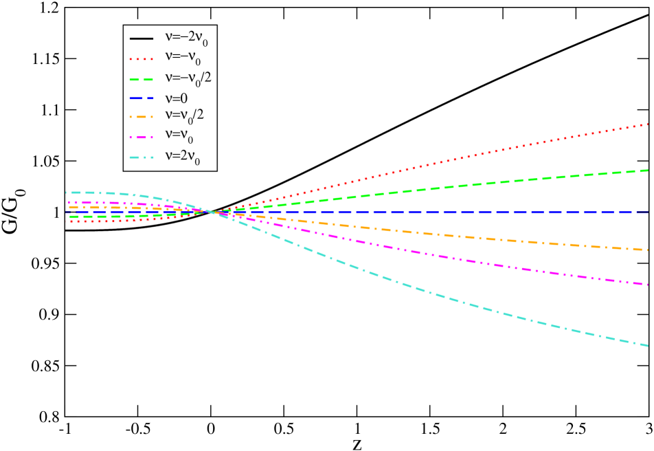
Figure 1: The dependence of the gravitational coupling constant $G=G(z;\nu)$ on the cosmological redshift $z$ for the six values (48) of the parameter $\nu$, where $\nu_{0}$ is given by Eq. (18). We assume a flat cosmology, $k=0$, with $\Omega_{M}^{0}=0.3$, $\Omega_{\Lambda}^{0}=0.7$. For the parameter values of the order $\nu_{0}$, there is a significant variation of $G$ at the redshifts amenable to high-z  SNe Ia observations.

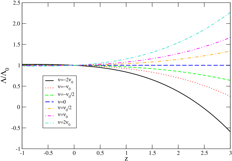
Figure 2: The dependence of the cosmological term energy density $\Lambda\equiv\rho_{\Lambda}(z;\nu)$ on the cosmological redshift for values of the parameter $\nu$ as in Fig. 1. For these parameter values there exists significant variation of $\Lambda$ (expressed in units of its present value $\Lambda_{0}\equiv\rho_{\Lambda}^{0}$) which may be detected by the high-z SNIa observations.

$$\delta_{\Lambda}(z;\nu)\equiv\frac{\delta\Lambda(z;\nu)}{\Lambda_{0}}=\frac{\Lambda(z;\nu)-\Lambda_{0}}{\Lambda_{0}}=\nu\,\frac{\Omega_{M}^{0}}{\Omega_{\Lambda}^{0}}\,\left[(1+z)^{3}-1\right]\,.$$ (46)

For convenience we have expressed the result in terms of the relative deviation of $\Lambda(z;\nu)$ with respect to the present value $\Lambda_{0}$, in order to better compare with Ref. [23, 24]. Amazingly, to first order in $\nu$, the cubic law (46) is identical to the one obtained in the latter references where a RG cosmological model with variable $\Lambda$ and fixed gravitational constant was considered. This means that the promising phenomenological analysis made in [24] concerning the redshift dependence of the cosmological constant remains essentially intact. Let us, however, mention that the two models depart from one another to second order in $\nu$. For the model under consideration we find

$$\delta_{\Lambda}(z;\nu)=\frac{\Omega_{M}^{0}}{\Omega_{\Lambda}^{0}}\,\left[(1+z)^{3}-1\right](\nu+\nu^{2})-\left[1+\frac{\Omega_{M}^{0}}{\Omega_{\Lambda}^{0}}\,(1+z)^{3}\right]\,\ln\left[\Omega_{M}^{0}\,(1+z)^{3}+\Omega_{\Lambda}^{0}\right]\,\nu^{2}\,.$$ (47)

To first order in $\nu$ we recover equation (46), and moreover we see that $\delta_{\Lambda}(0;\nu)=0$ for any $\nu$, as it should be.

The previous (approximate) results are confirmed and refined through a numerical analysis of the exact formulas (42)-(44). We take as representative values of $\nu$ some multiples of the typical value $\nu_{0}$, Eq. (19). Specifically, we consider the six cases with different signs represented by the $\nu$-data row:

$$\overrightarrow{\nu}=\left(-2\nu_{0},-\nu_{0},-\frac{1}{2}\,\nu_{0},+\frac{1}{2}\nu_{0},+\nu_{0},+2\,\nu_{0}\right)\,.$$ (48)

The results are presented in Fig. 1 and 2 for the standard values of the cosmological parameters [2]: $\Omega_{M}^{0}=0.3$, $\Omega_{\Lambda}^{0}=0.7$. Specifically, in Fig. 1 we plot the exact function $G=G(z;\nu)$ for the six values of $\nu$ listed above. Similarly, in Fig. 2 we plot the function $\Lambda=\Lambda(z;\nu)$ for the same values of the $\nu$ parameter. We have verified these results also by direct numerical solution of the differential equations using Mathematica [47]. By looking at Fig. 1 we may read off the relative correction $\delta_{G}$ on $G$. We see, for example, that significant corrections $\delta_{G}\simeq-5\%$ are predicted at redshift $z=1.5$, if $\nu\simeq\nu_{0}$. Furthermore, for the same values of $\nu$ and $z$, we find $\delta_{\Lambda}\simeq 16\%$ (cf. Fig. 2). This correction to $\Lambda$ should be perfectly measurable by SNAP[43]. Recall that this experiment aims at exploring cosmological depths up to $z=1.7$, and that other experiments are planning to go even beyond (including the HST) [48].

We should point out that cosmological corrections to $G$ of a few percent at high redshifts are not in contradiction to present bounds on the gravitational constant [49, 50]. The reason is that the existing bounds are “local”, i.e. at the scale of the Solar System, so that they do not provide any information on possible variations of $G$ at cosmological distances. Actually it is difficult to measure the correction $\delta_{G}$ at the cosmological level, at least in the present matter-dominated epoch. There is no direct way to measure $G$ at distances of hundreds to thousands of Megaparsecs, unless we re-interpret the observed cluster dynamics in terms of $G$ variation on a cosmological level, rather than in terms of CDM. We will further elaborate on this kind of idea in the next section, but restricting ourselves for the moment to the more familiar galactic domain. On the other hand, if we extrapolate back our running formula for $G$ to the radiation epoch we might expect to find some additional information. Particularly relevant is the nucleosynthesis epoch ($z\sim 10^{9}$). Performing the corresponding change $\rho_{M}\rightarrow\rho_{R}$ in Eq. (43), with $\rho_{R}(z)=\rho_{R}^{0}\,(1+z)^{4}$, we find that for $\nu$ of order $10^{-2}$ the relative variation $\delta_{G}$ lies within the limits set by the latest analyses on $G$ variation at nucleosynthesis, which give a margin of $\sim 40\%$ at the $95\%$ C.L. [51] Thus the existing nucleosynthesis limits placed on $\nu$, based on considerations on $\Lambda$ variation alone [23, 24], are essentially unchanged.

7 A possible application to flat rotation curves of galaxies

In this section we speculate on the possibility to apply similar RG methods to the more restricted astrophysical domains, such as the galactic scales. While we have seen that it is difficult to measure the correction $\delta_{G}$ at the cosmological level, let us explore the possibility to measure local variations of the gravitational constant (induced by the RG) at the level of a typical galaxy, and extract some potential consequences concerning the origin of the flat rotation curves in its halo – usually associated to the presence of undetected CDM [1] . Here again the main question is to identify the scale of the RG. It can no longer be $\mu\simeq H$ because measurements within our galaxy are not cosmological measurements, just astrophysical. Indeed, $H$ does not change on the scale of a galaxy (a bound system!). However, if $G$ varies according to some RGE, there must be some new order parameter for the local RG scale. For simplicity let us treat the galaxy as a central core surrounded by a spherically symmetric mass distribution. Then, from simple dimensional arguments we may assume that the appropriate RG scale for the galactic dynamics is given by

$$\mu=\frac{\kappa}{r}\,,$$ (49)

where $\kappa$ is some (dimensionless) constant and $r$ is the radial distance (in the “renormalized metric”, see below) measured from the center of the galaxy. If we assume that the renormalization effects from the RG are small enough (after all they cannot change dramatically the Newtonian picture), we may take $r$ as the standard radial coordinate in classical celestial mechanics. Notice that $\mu$ can never go smoothly to zero because $r$ is bounded from above. This means that at the galactic level we do not expect that the corresponding expansion $G(\mu)^{-1}$ in (13) is analytic near $\mu=0$ because the system is intrinsically finite-sized. However, by artificially extending the size of the local system we expect that the same IR behavior of the cosmological case mentioned in Section 5 should be encountered. This provides a connection between the two regimes (local and cosmological) that can be used to establish the consistency of the RG application to the local case. The Ansatz (49) obviously implies that spatial gradients of $G$ (and may be also of $\Lambda$) are allowed. It should be clear that this is not in conflict with the Cosmological Principle because the latter applies to the Universe in the large, not to local systems such as galaxies or clusters of galaxies . Although the Ansatz (49) is plausible, we may try to motivate it from the point of view of the scale setting procedure (25). Strictly speaking, the latter has been rigorously formulated only for the transition from the cosmic time evolution to scale evolution. However, given the fact that at very large scales $r$ is of order of the horizon, $1/H$, we see that with the hypothesis (49) the original scale setting used in previous sections, $\mu\simeq H$, is consistently met on cosmological scales. Consider the typical density profile for flat rotation curves:

$$\rho(r)=\frac{\rho_{0}}{1+(r/r_{0})^{2}}\,.$$ (50)

Here $r_{0}$ is a reference galactic length of the visible part of the galaxy; e.g. in the case of our galaxy it can be taken as the “local” position (at the galactic scale) of our Solar System, where the gravitational constant is supposed to be $G_{0}$ essentially everywhere, and $\rho_{0}$ is the average density of the galaxy well before reaching the halo regime. Clearly $\rho(r)\rightarrow\rho_{0}$ for $r\ll r_{0}$ whilst $\rho(r)$ falls off as $1/r^{2}$ for $r\gg r_{0}$ (i.e. deep in the halo). This behavior is exactly what is needed to have a linear growth of the galactic mass deep in the halo region,

$${\cal M}(r)=\int_{r\gg r_{0}}d^{3}r\ \rho(r)\propto r\,,$$ (51)

and therefore a constant rotation velocity in it:

$$v=\sqrt{\frac{G\,{\cal M}(r)}{r}}\rightarrow{\rm const.}$$ (52)

This is the classical “explanation” for the flat rotation curves, once the galactic density profile (50) is accepted by fiat. One possibility (the most commonly accepted one) is that (50) is associated to the presence of CDM distributed in the halo region $r\gg r_{0}$. However, an alternative justification for this density function (and perhaps also the ultimate origin of the flat rotation curves) could actually be linked to the RG running of the gravitational constant as a function of the new scale parameter (49). A hint that this could be the case is obtained by substituting the density (50) into $\rho$ in Eq. (40). It is easy to see that when the halo regime sets in, the resulting formula behaves precisely in the form (49). We will see below that the density (50) although it is not the real mass density of the galaxy in our framework (because we do not assume a priori the existence of CDM), it can be reinterpreted as the “renormalized” mass density, i.e. the “effective mass density” of the galaxy after considering the renormalization effects on Newton’s gravitational constant. In this sense it is this expression that must be used to determine the RG scale. Let us therefore take these features as heuristic motivations to adopt $\mu$ from (49) as a valid RG scale for the galactic regime, and let us explore the ensuing consequences within our RG framework. Upon replacing $\mu=H$ with $\mu=\kappa/r$ and $H_{0}$ with $\kappa/r_{0}$ in our running formula (33) we find

$$G(r)=\frac{G_{0}}{1+\nu\,\ln\left(r_{0}^{2}/r^{2}\right)}\,.$$ (53)

We assume $\nu>0$ in (53) so that $G$ is asymptotically free, and therefore it increases with $r$. This kind of growing behaviour of $G$ with the distance is reminiscent of the above mentioned possibility that gravity can lead to non-perturbative effects in the far IR. The running of $G(r)$ in the surroundings of the Solar System (i.e. for $r\simeq r_{0}$) is very small; in practice there is no running at all, for the entire Solar System is represented by the point $r=r_{0}$ without extension. This insures that we normalize our $G_{0}$ above with the value obtained from highly accurate measurements of $G$ performed in our neighborhood [49, 50]. Any departure from this value was never accessible to us because we never measured $G$ (at least directly and accurately) outside the Solar System. Moreover, the formula above cannot be applied for $r$ near $r=0$. The reason is that the geometry is governed by the Schwarzschild metric (see below), and therefore there is an event horizon at some point $r=2\,G{\cal M}\ll r_{0}$, where ${\cal M}$ is the mass of the galaxy concentrated at its center. We can only assume valid Eq. (53) well beyond this limit. Next we consider the modified Einstein-Hilbert action with variable $G$:

$$S^{(1)}_{EH}=-\int d^{4}x\sqrt{-g}\,.\frac{R}{16\pi\,G(r)}\,.$$ (54)

If G were constant, we would expect that the metric that solves the galactic dynamics at large $r$ is the spherically symmetric Schwarzschild metric. For variable $G$, however, the situation is more complicated. One could vary the action (54) and try to find out the field equations, but it is hard to solve them exactly. Whatever the solution is, at least we know that the spherical symmetry must still be there. Therefore, in the absence of an exact result we may use the fact that $G(r)$ is given by (53) and that $\nu$ is a small parameter. Following the conformal symmetry methods of [54, 13], we introduce the auxiliary action

$$S^{(2)}_{EH}=-\frac{1}{16\pi G_{0}}\,\int d^{4}x\sqrt{-\bar{g}}\,\,\bar{R}\,,$$ (55)

with respect to the auxiliary metric $\bar{g}_{\mu\nu}$, and with constant $G=G_{0}$. This action transforms into the action

$$S^{(3)}_{EH}=-\frac{1}{16\pi G_{0}}\,\int d^{4}x\sqrt{-g}\,\,e^{2\,s}\left[\,R+6\,(\partial s)^{2}\,\right]\,.$$ (56)

under the local conformal transformation

$$\bar{g}_{\mu\nu}=e^{2s}\,{g}_{\mu\nu}\,,$$ (57)

where $s=s(r)$ is a function of $r$. With this trick, let us now choose the following conformal factor:

$$e^{2s}=\frac{G_{0}}{G(r)}={1+\nu\,\ln\left(r_{0}^{2}/r^{2}\right)}\,,$$ (58)

where $G(r)$ is given by (53). Then the action (56) becomes the $r$-dependent G action (54) except for the extra derivative terms $(\partial s)^{2}$:

$$S^{(4)}_{EH}=-\int d^{4}x\sqrt{-g}\,\frac{R}{16\pi\,G(r)}-6\int d^{4}x\sqrt{-g}\,\,\frac{(\partial s)^{2}}{16\pi\,G(r)}\,.$$ (59)

Notice that the square derivative terms are of higher order in $\nu$ with respect to the Lagrangian density $\sqrt{-g}\,R/G(r)$, and can be neglected. Indeed, differentiating (58) on both sides gives $e^{2s}\partial s/\partial r=-\nu/r$ and hence the square derivative that appears as the extra term in (59) becomes of order $(\partial s)^{2}\sim\nu^{2}/r^{2}$. For a typical radius $r$ comparable to the galactic size we can fully neglect this term as compared to $R\sim 1/r^{2}$ because contributions of order $\nu^{2}$ are very small. It follows that the solution of the field equations associated to the original action (54) with variable $G$ is, to first order in $\nu$,

$$g_{\mu\nu}=e^{-2s}\,\bar{g}_{\mu\nu}=\left(1+2\nu\ln\frac{r}{r_{0}}\right)\,\bar{g}_{\mu\nu}\,.$$ (60)

From the arguments above, $\bar{g}_{\mu\nu}$ must be the solution of the ordinary Einstein equations with constant $G_{0}$ corresponding to the galaxy system treated as a point-like core of mass ${\cal M}$. Therefore $\bar{g}_{\mu\nu}$ on the r.h.s. of (60) must necessarily be the standard Schwarzschild metric corresponding to constant $G_{0}$:

$$ds^{2}_{\rm Schw}=\left(1-\frac{2\,G_{0}\,{\cal M}}{r}\right)\,dt^{2}-\frac{dr^{2}}{1-2\,G_{0}\,{\cal M}/r}-r^{2}\,d\Omega^{2}\,.$$ (61)

From (60) we learn that the solution of the field equations for $G=G(r)$ must be a modified (or “renormalized”) Schwarzschild’s metric. To first order in $\nu$ the renormalization amounts to the new line element

$$ds^{2}=\left(1+2\nu\ln\frac{r}{r_{0}}\right)\,ds^{2}_{\rm Schw}\,.$$ (62)

Let us now take the $g_{00}$ component of this modified metric and recall that the classic potential $\Phi$ is identified from $g_{00}=1+2\Phi$. To first order in $\nu$ it reads

$$\Phi(r)=-G_{0}\,\frac{\cal M}{r}+\nu\,\left(1-2\,G_{0}\,\frac{\cal M}{r}\right)\,\ln\frac{r}{r_{0}}\,.$$ (63)

The corresponding force per unit mass becomes

$$F(r)=-\frac{d\Phi}{dr}=-(1-2\,\nu)\,G_{0}\,\frac{\cal M}{r^{2}}-\,\nu\,\left(\frac{1}{r}+\,G_{0}\,\frac{\cal M}{r^{2}}\,\ln\frac{r^{2}}{r^{2}_{0}}\right)\,.$$ (64)

This intriguing result shows that for sufficiently large $r$ (namely, in the halo of the galaxy where $r>>r_{0}$) the force that we have found is not purely Newtonian as it does no longer decay as $1/r^{2}$ at high distances, but as $1/r$. The coefficient of the $1/r$ term is precisely the parameter $\nu$ of our renormalization group model. Equating this force to the centripetal force $-v^{2}/r$ and neglecting for the moment the $1/r^{2}$ (Newton’s) term and the $(\ln r)/r^{2}$ term, one finds that for large $r$ the rotation velocity is virtually constant, i.e. it does not depend on $r$ (the rotation curve becomes flat). Such asymptotic velocity is thus determined in good approximation by the square root of our original parameter $v=\sqrt{\nu}$. In conventional units the velocity reads $v/c=\sqrt{\nu}\$. Of course we expect $v/c<<1$ for any rotating object in the halo. But this can be well accomplished through the coefficient $\nu$, which was always expected small in our effective field theory approach to the $\beta$-function of $\Lambda$ down the Planck scale, see (18). We argued that $\nu$ could typically be of order $10^{-2}$ for the cosmological considerations. However, we may ask now: how much small must it be to describe the physics of the flat rotation curves of galaxies? The rotation velocities in most galaxies are of a few hundred Km/s, say $200-300$ Km/s [1]. It follows that if this model is to describe them, $\nu$ should be of order

$$\nu\sim 10^{-6}\,.$$ (65)

Obviously a very small value! It implies that all of the approximations that we have made for $\nu\ll 1$ should be perfectly acceptable. And of course, from the cosmological point of view, it is neatly compatible with the CMB and LSS measurements  [46]. With this value of $\nu$ we may explicitly check that the dominance of the leading extra term $\nu/r$ in (64) over the Newtonian one, $G_{0}\,{\cal M}/r^{2}$, really takes place in the halo of the galaxy, where $r>>r_{0}$. Indeed, for a typical galaxy with a mass $10^{10-11}$ times the mass $M_{\odot}$ of our Sun, and with the $\nu$ value (65) obtained in our RG framework, it is easy to check that the $\nu/r$ term is comparable to the Newtonian force just around a scale of several to ten $Kpc$, namely near the onset of the halo region. Beyond $10\,Kpc$, and of course deep in the halo region, the “$\nu$-force” is dominant.

If we keep the other terms in (64), except for the very small correction to the Newtonian part of the force, we find the following formula for the flat rotation velocity:

$$v/c=\sqrt{\nu+\,G_{0}\,\frac{\cal M}{r}\left(1+\nu\,\ln\frac{r^{2}}{r^{2}_{0}}\right)}\simeq\sqrt{\nu+\,G_{0}\,\frac{\cal M}{r}}\,,$$ (66)

where in view of the small value (65) we have neglected $\nu\,\ln(r^{2}/r^{2}_{0})\ll 1$. The previous result reads essentially $v/c=\sqrt{\nu}$ up to a small correction which depends on the total mass of the galaxy and the radial distance to the rotating object in the halo. This is again an interesting feature, because the velocity of the flat rotation curves is well-known to show some departure from universality [1]. In fact, we can further shape this formula such that it becomes closer to the observed behavior. From the modified Newton’s law we may estimate the effective mass (or “renormalized mass ${\cal M}_{r}$”) of the galaxy associated to the renormalization of $G$. By equating the purely Newtonian term in (64) to the leading correction proportional to $\nu$ we immediately conclude that the “effective additional mass” of the galaxy is proportional to $r$ in the halo region,

$$\delta{\cal M}(r;\nu)\simeq\left(\frac{\nu}{G_{0}}\right)\,\,r\ \ \ \ (r\gg r_{0})\,.$$ (67)

The total renormalized mass of the galaxy (the one which is actually observed, if one adopts the purely Newtonian approach) is thus given by the “bare mass” (i.e. the “real” or ordinary mass ${\cal M}$ made out of baryons) plus the renormalization effect computed above: ${\cal M}_{r}={\cal M}+\delta{\cal M}$. It should, however, be clear that this is a huge renormalization effect, because $\delta{\cal M}$ is comparable to (actually larger than) ${\cal M}$ as it could be expected from the fact that, in the language of the CDM, the extra amount of matter in a typical galaxy is known to be dominant over the luminous one: roughly ten times the total baryonic matter (whether luminous or not). It means that we should have $\delta{\cal M}\gg{\cal M}$, equivalently ${\cal M}_{r}\simeq\delta{\cal M}$. This feature is nicely realized in our RG framework and again emphasizes the potential non-perturbative character of the gravitational effects in the IR regime, similar to the strong low-energy dynamics of QCD. To see this quantitatively, let us take $r$ deep in the halo region, say in the range $10-50\,Kpc.$, and let us assume a galaxy with a physical mass ${\cal M}=10^{10}\,M_{\odot}$ (typically the case of the total baryonic mass of our galaxy). It is easy to estimate from (67), using the value of $\nu$ given in (65), that $\delta{\cal M}\simeq 10\,{\cal M}$, which is in the right order of magnitude to describe a total effective mass around ${\cal M}_{r}\sim 10^{11}\,M_{\odot}$ without invoking the existence of CDM. Strictly speaking, there is no physical halo in the RG approach, but at some point the local RG description must break down. This should define an “effective RG halo” of the galaxy, beyond which a larger scale RG picture should take over.

The linear growth of the mass given in Eq.  (67) implies that the “effective density” of the galaxy in the halo region behaves as

$$\rho(r)\simeq(\frac{\nu}{4\,\pi\,G_{0}})\,\left(\frac{1}{r^{2}}\right)\ \ \ (r\gg r_{0})\,.$$ (68)

This effective density replaces the material effects associated to the CDM matter density (50). Comparing both densities in the region $r\gg r_{0}$ we obtain $r_{0}^{2}\,\rho_{0}=\nu/4\pi G_{0}$. Setting $\rho_{0}\sim{\cal M}/r_{0}^{3}$ we have ${\cal M}/r_{0}\sim\nu/G_{0}$, which is indeed satisfied within order of magnitude for a similar set of inputs as before. Finally, since the renormalized mass of the galaxy is proportional to the galactic radius in the halo region, we conclude that the rotation velocity (66) can be cast as

$$v(r;{\cal M})/c\simeq\sqrt{\nu}\,\left[1+\varepsilon(r;{\cal M})\right]^{1/2}\ \ \ \ (r\gg r_{0})\,,$$ (69)

where $\varepsilon(r;{\cal M})$ is a small correction that exhibits the departure of the flat rotation curves from universality. It reads

$$\varepsilon(r;{\cal M})=\frac{{\cal M}}{{\cal M}_{\nu}(r)}\,,$$ (70)

with ${\cal M}_{\nu}(r)\equiv\delta{\cal M}(r;\nu)$ given by Eq. (67). Notice that ${\cal M}_{\nu}(r)$ does not depend on the mass of the galaxy, but only on $\nu$ and on the radial position of the rotating object. We have seen above that typically ${\cal M}_{\nu}(r)\sim 10\,{\cal M}$ for $r\gg r_{0}$. Therefore, we conclude that the flat rotation velocity becomes a function $v=v(r;{\cal M})$. In other words, the small corrections to universality depend on the mass of the galaxy and of the radial location of the object, another observed feature. Only further refinements of the RG approach and the galaxy model may perhaps shed some light on the detailed numerical predictions concerning the value of the rotation velocity and its dispersion. Our formula above can easily accommodate velocity dispersions of order $10\%$. However, we cannot expect perfection. Recall that we modeled the galaxy as a spherical distribution of matter while it is roughly disk-shaped, thus other geometric and dimensionful variables might enter (including the mass ${\cal M}$ of the galaxy) to refine our scale Ansatz (49). This could have some further impact in the departure of the flat rotation velocity from universality.

We should recall that the flat rotation curves of the galaxies can be fitted within the Modified Newtonian Dynamics (MOND) [55]. This phenomenological model requires gravitation to depart from the standard Newtonian theory in the extra-galactic regime ($r\gg r_{0}$). The MOND potential takes the form

$$\tilde{\Phi}(r)=-G_{0}\,\frac{\cal M}{r}+\sqrt{a_{0}\,G\,{\cal M}}\ \ln\frac{r}{r_{0}}\,.$$ (71)

The structure of the extra-galactic modification (the second term) is such that one can fit both the flat rotation curves and the departure of these curves from strict universality. The first feature is achieved from the logarithmic form of the correction, and the second feature is implemented by allowing for the coefficient of the logarithm to depend on the product $G\,{\cal M}$, where ${\cal M}$ is the mass of the galaxy. Obviously the overall coefficient must be dimensionless, and therefore one is forced to introduce a new “fundamental acceleration” parameter $a_{0}$ in Eq. (71), which can be fitted observationally to a value of order $10^{-8}\,cm\,sec^{-2}$. The combination of these two features is all what is needed to simultaneously account for the leading and subleading observational effects of the galaxy rotation curves without invoking the existence of CDM haloes: to wit, the flatness of these rotation curves and the so-called Tully-Fisher’s law, $v^{4}\propto{\cal L}$, where $v$ is the asymptotic value of the rotation velocity and ${\cal L}$ is the absolute luminosity of the galaxy [56]. This law expresses some departure of the flat rotation curves from universality and can be rephrased in terms of the mass of the galaxy. If one makes the standard assumption that the mass-to-light ratio, ${\cal M}/{\cal L}$, is essentially constant for spiral galaxies, then $v^{4}\propto{\cal M}$. MOND indeed implements this relation in the form $v^{4}=a_{0}\,G\,{\cal M}$ – as it trivially follows from (71). However, it must be clearly stated that in spite of the great phenomenological success of MOND, so far none of the relativistic gravitational theories proposed up to date (aiming to underpin that phenomenological model from first principles) can be considered as free of theoretical and experimental inconsistencies, including the recent attempt in  [57]. In this sense, it is a welcome feature that we can derive the leading effect (the existence of the flat rotation curves themselves) from our RG framework. This is obvious when we compare our modified Newtonian potential (63) and the MOND potential (71). The two potentials have in common the necessary logarithmic term to account for the leading correction to Kepler’s law entailing the flat rotation feature. However, the RG-inspired potential (63) does not lead to the (subleading) Tully-Fisher’s effect, while the MOND potential contains the piece $\sqrt{a_{0}\,G\,{\cal M}}$ just ordered ad hoc to reproduce this additional feature. It could be that the RG-potential misses this piece due to the simplifications we have made to reach the leading result. We hope that further investigations will help to clarify this issue. In the meanwhile Eq. (70) above already suggests that some mass-dependent departure from universality is predicted in the simplest RG approach.

With $\nu$ as small as (65) the increase of $G(r)$ from (53) remains negligible, even at cosmological distances. Therefore, it is conceivable that $G(r)$ essentially behaves as a constant, with no further significant variation up to the horizon. At this point we recall that the motivation for (53) was, in contrast to the more formal one of (33), essentially heuristic. However, since at very large scales $r$ is of order of the horizon, $1/H$, the function $G=G(r)$ merges asymptotically with $G=G(H)$. In this way the original scale setting $\mu=H$ is retrieved on cosmological scales and there is a matching of the two scale settings in the asymptotic regime. Notwithstanding, we should clarify that we do not expect a sharp transition from one RG regime to the other; we rather expect the existence of some interpolating RG description that connects scales of order $100\,Kpc$ (which characterizes the maximum expected size of the galactic haloes) with scales of order $100\,Mpc$ (above which the large scale cosmological picture takes over). In the crossover region the effective density (68) should fall off faster than $1/r^{2}$. Unfortunately, it is not possible to be more quantitative here on the specific form of this transition, but we do expect it should be there. After going through this transition the running formula (53) becomes (33) and the common, and essentially constant, value of $G$ in the two scaling laws represents the cosmological value of the gravitational constant. The only measurable effect left in this scenario would be the aforementioned correction to Newtonian celestial mechanics, which could have an impact on dark matter issues at the galactic and even at larger (cluster) scales. But we are not going to push further this possibility here nor to contemplate the possibility of other refinements. In particular, in the above considerations we have ignored the potential running effects from the cosmological constant at the galactic scale, which were assumed to be small. We close this section by noticing that with $\nu$ of the order of (65), the GUT scale potentially associated to these quantum effects would be $M_{X}\sim 10^{16}\,GeV$ rather than $10^{17}\,GeV$ (see Eq. (22)), therefore closer to the lowest expected SUSY-GUT scale.

8 Discussion and conclusions

In this paper we have further elaborated on the formulation of the renormalization group cosmologies along the lines of  [7, 21, 22, 23, 24, 32, 33, 36]. The main aim of these RG cosmologies is to provide a fundamental answer, within QFT, to the meaning of the most basic cosmological parameters such as $H_{0}$, $G$, $\rho_{M}^{0}$ and $\Lambda_{0}\equiv\rho_{\Lambda}^{0}$, and at the same time to try to understand their presently measured values and possible interrelations among them. In doing so we have found that the classical FLRW cosmologies become “renormalization group improved”, and therefore they become slightly modified by quantum corrections associated to renormalization group equations that govern the evolution of the parameters $\Lambda$ and $G$. This evolution behaviour, primarily a scaling one within the framework of the RG, can be inter-converted into a temporal evolution (i.e. in terms of the cosmic time or, if desired, in terms of the redshift), after an appropriate identification of the scale parameter $\mu$ of the RG. We have found that $\mu\sim H(t)$ is a consistent identification for the class of RG cosmologies in which $\Lambda$ evolves quadratically, and $G$ evolves logarithmically, with $\mu$. And we have shown that this combination of running laws is a most promising one from the point of view of phenomenology. The scaling (and redshift) variation of these two laws is very simple and it is controlled by a single parameter, $\nu$ – cf. Eq. (18). For $\nu>0$ the running law for the gravitational constant exhibits (logarithmic) asymptotic freedom, much as the strong coupling constant in QCD. For $\nu\ll 1$ the quadratic evolution law for $\Lambda$ turns out to be very similar to the one previously found in [23, 24] and therefore it can be tested in the future experiments by SNAP [43], provided $\nu$ is not much smaller than $\nu_{0}\sim 10^{-2}$. This value is presently consistent with data from high-z SNe Ia, CMB and LSS. Furthermore, from the point of view of the cosmological constant problem, we have seen that this RG framework can shed some light to the coincidence cosmological problem ($\rho_{\Lambda}^{0}\simeq\rho_{M}^{0}$ ?) because it provides a natural explanation of the puzzle of why the energy scale associated to the cosmological constant is at present the geometric mean of the Hubble parameter and the Planck mass: $E_{\Lambda}(t_{0})\simeq\sqrt{M_{P}\,H_{0}}$.

It is important to remark that the quadratic law (16) associated to our RG framework is not just a proportionality law $\Lambda\sim H^{2}$, but a variation law: $\delta\Lambda\sim H^{2}$. In contradistinction to the former, the latter actually introduces an additive term. This is because it originally comes from a RGE of the form $d\Lambda/d\ln H\propto H^{2}$, which has to be integrated, see Eq. (14). Therefore the ensuing cosmologies are very different from the $\Lambda\sim H^{2}$ ones. Only the latter have been amply discussed in the past in many places of the literature [19, 20], including some recently raised criticisms [42, 58]. In contrast the $\delta\Lambda\sim H^{2}$ law is, to the best of our knowledge, relatively new in the literature [7], and its motivation within QFT gives it a credit at a much more fundamental level. Let us mention that some variation of this law has been proposed very recently (on pure phenomenological grounds) in [42], in the form $d\Lambda/da\propto dR/da$, where $R$ is the curvature scalar. However, since $\mu=R^{1/2}$ is, as mentioned above (and in [7]), a covariant generalization of $\mu=H$, it is essentially the same law and so the conclusions are similar. Therefore the RG cosmologies associated to $\delta\Lambda\sim H^{2}$ can also be formulated covariantly, without committing to the particular FLRW metric. But from the practical point of view (and also to better assess its physical meaning and potential applications [24, 33]) it is better to formulate this law making use of the Hubble parameter, instead of curvature.

The last part of our paper is more speculative. We have tantalized the possibility of extending the RG formalism to local cosmological domains such as the galactic level. After arguing that the local RG scale could naturally be $\mu\sim 1/r$, we have solved the modified Schwarzschild metric in the limit $\nu\ll 1$ and derived a RG correction to Kepler’s third law of celestial mechanics. We have hypothesized that this quantum correction could furnish an explanation for the flat rotation curves of the galaxies, provided $\nu\sim 10^{-6}$. Obviously, this possibility would exclude measurable effects on the cosmology side, where a larger $\nu$ is needed, but it might hit square on one of the biggest astrophysical conundrums of the last thirty years. This result is curious enough and rather intriguing, and we have found interesting to include it as an additional potential application of our RG framework. All in all, we deem this last part of our work more speculative than the rest, because we have had to descend from the cosmological level to the (more complicated) local domain where cosmology is entangled with astrophysics, and other factors may come into play. Thus, more detailed theoretical considerations are needed to formally establish the RG effects at the galactic level, which could be modified by other factors such as the modeling of the galaxy and the details of the RG framework. For this reason, even if $\nu$ is of order of $\nu_{0}$, and therefore much larger than (65), the corresponding RG predictions at the galactic level are not necessary in contradiction with the experimental situation. The actual effects could be much smaller due to, say, the need to introduce some significant modification in the Ansatz (49), as noted in the last section. Finally, even if accepting that $\nu$ is small enough for the RG to be able to provide some explanation of the flat rotation curves, it does not preclude the possibility that galactic dark matter is present in the haloes of the galaxies. It only shows that other, even more subtle, effects could creep in. Whether or not these effects are directly related to the RG must be further investigated, but already at the pure phenomenological level the possibility that a logarithmic law of the type (53) could be behind the flat rotation curves looks rather enticing. Obviously, even if it is not the sole explanation, it may help to reduce the total amount of dark matter needed to account for the flat rotation curves and also to explain some features related to the deviation from universality of the flat velocities. In any case it is clear that further experimental work will also be necessary to decide on the ultimate origin of the rotation curves of the galaxies [59]. In general, even if letting aside the possibility of these local effects, our cosmological RG framework provides a sound alternative to explain the nature of the cosmological parameters and their potential connection to quantum field theory. It also offers a link between the low-energy physics characteristic of large scale Cosmology with the high-energy interactions of Particle Physics. Last, but not least, it constitutes a ready testable framework for the next generation of cosmological experiments.

Note Added: Shortly after the e-print Archive version of this paper was submitted as hep-ph/0410095, some other works were submitted to the Archive – see [60, 61]– which overlap significantly with the content of Section 7. These works also use the RG to study the flat rotation curves of the galaxies and arrive to conclusions very similar to the ones presented here. Since, however, their approach is different from ours we think it can be useful for the reader if we comment on the similarities and also the main differences between the two methods.

First of all we recall that two Renormalization Group formulations for gravity are present in the literature, namely the perturbative RG for curved space-time and the Wilsonian non-perturbative RG for quantum gravity. The present work is based on the first of these RG approaches (see [27, 28] for an introduction and references). The object of our interest is the quantum theory of matter fields on classical curved background. It is very important that this theory is renormalizable and therefore application of the perturbative RG to this case is a consistent procedure. Unfortunately, the consistency does not mean that this approach does not meet real difficulties. The existing well-established formalism is essentially restricted by the $\overline{\mbox{MS}}$-scheme of renormalization. Within this approach one can learn how the observables dependent on the dimensional parameter $\,\mu$, but the physical interpretation of this parameter always requires a special additional effort. Furthermore, the $\overline{\mbox{MS}}$-scheme is reliable only in the UV limit and is not appropriate for the investigation of the relatively weak IR scaling, that is for the study of decoupling. An alternative mass-dependent scheme has been recently applied in curved space-time, but only in the particular case of linearized gravity [37]. In this case we can observe the Appelquist&Carazzone decoupling theorem [45] to hold in the higher derivative sectors of the gravitational action. The present and previous [7, 22, 23, 24] works are based on the phenomenological assumption that a similar kind of decoupling behaviour takes place for the cosmological constant. One can find an extended discussion of this issue in the Appendix A of [24].

On the other hand, the alternative works [60] (exactly as the previous ones [25, 26], see further references therein) deal with the IR effects of quantum gravity. It is well known that quantum gravity is inconsistent within the perturbative approach and hence the appropriate version of the RG is necessarily non-perturbative. Ref. [60] is based on a simplified version of the Wilsonian approach to this non-perturbative RG framework. The objective is the derivation of the functional of the flow effective action, depending on the cut-off parameter $\,k$. This parameter can be viewed as a direct analog of the parameter $\,\mu\,$ for the perturbative RG in the $\overline{\mbox{MS}}$-scheme. The main similarity between the two parameters is that one also needs to properly identify $\,k\,$ with certain physical quantity (e.g. the energy of the gravitational quanta or the inverse of the cosmic time $\,t$). Without such identification the theory has no physical output. The choice of the scaling parameter in both RG approaches is not constrained by the RG formalism itself, and in certain (sufficiently simple) situations it can be guessed on the basis of physical (e.g. dimensional) arguments. This is the case when the system has just one relevant physical scale. For instance, in the astrophysical case under consideration in Section 7 the galaxy is assumed to have spherical symmetry and then the single relevant physical scale is the radial distance $r$ from its center. This leads to the successful scale choice (49). On the other hand, in the cosmological context, a possible way of constraining the scale setting is the procedure applied in Section 4. This leads immediately to our choice $\mu=H$ – cf. Eq. (31) – roughly consistent with the scale setting $k\sim 1/t$ advocated in the alternative RG approach of [60]. However, even this regular procedure does not obviously provide universal solution for all physical situations (for example, in multiple scale systems or in the transition from the cosmological to the astrophysical domain). Therefore, the link between the RG running and the $\,r$-dependence in the astrophysical setting is an essentially phenomenological assumption for both RG formulations, and needs further investigation.

As we already mentioned above, in our RG approach we assume the standard form of decoupling for the cosmological constant. Similarly, the alternative RG approach – the Wilsonian non-perturbative formulation of the RG for quantum gravity – requires also of strong phenomenological input. In the Wilsonian version of the RG used in [60] the effective action depends on infinitely many couplings associated to powers of curvature and non-local invariants. Solving the exact functional RG flow equation is virtually impossible at present and in practice one truncates this effective action into a linear combination of powers of curvature, the simplest possibility being the powers one and zero, i.e. the Einstein-Hilbert term and the cosmological term. The coefficients of these terms define the flow trajectory $(G(k),\Lambda(k))$ projected onto this simplified finite-dimensional space.

However, by virtue of this simplification the flow trajectory $G=G(k)\,,\Lambda=\Lambda(k)$ cannot be derived from the RG flow equation, and therefore an Ansatz on the trajectory is to be made in general. For the galactic problem at hand, one typically dismisses the role played by the cosmological term and is left with proposing an (ad hoc) modeling for the $G$ flow. The model trajectory explored in  [60] reads $G(k)=1/k^{q}$ (with $q$ an arbitrary parameter). In order to describe the flat rotation curves the authors of [60] have to take for $q$ a very small value of order $10^{-6}$. In contrast, in a previous paper [26] it was assumed the particular value $q=2$ in order to describe a RG cosmology with a (hypothetical) IR fixed point. Obviously this trial and error strategy shows that the state of the art in the RG flow effective action approach is not good enough at present as to allow for determining the flow trajectory $G=G(k)$ in a fully dynamical way. It is nevertheless remarkable that after accepting the value $10^{-6}$ the previous power law trajectory becomes effectively a logarithmic running law, which is entirely similar to the one we have obtained in Eq. (53) on a very different basis.

Comparing the merits of the two RG approaches we can indicate two advantages (from our point of view) of the one considered in the present paper. First, we are dealing with the quantum effects of matter fields, which definitely take place. The necessary phenomenological implication concerns only the technical (albeit serious) difficulty of evaluating the vacuum effective action of massive fields on a curved background. In contrast, the relevance of the quantum gravity effects and the possibility of their description without solving the fundamental problem of quantum gravity looks rather uncertain. This concerns both the method of Ref. [60] and the one of the old works [52] where the perturbative higher derivative quantum gravity effects were considered (and similar results were obtained). Second, the present approach has at least the virtue of introducing a parameter, $\nu$, whose definition (namely, $\nu$ is the ratio of the masses squared of the heavy matter fields versus the Planck mass squared, see Eq. (18)), naturally fits in the right order of magnitude to explain the effect. At then end of the day, since both approaches are essentially based on phenomenological input, the preference of one of them remains a matter of taste. However, the net outcome is that the running law (53) and the one found in [60] are identical if one identifies $q\equiv 2\,\nu$ in the limit of very small value of these parameters (the only relevant limit for the galactic dynamics).

Let us also mention a recent modification of the RG approach, the so-called metric-skew-tensor-gravity theory proposed in [61]. Here a skew-symmetric field tensor $F_{\mu\nu\lambda\sigma}$ is introduced and coupled to matter. This model introduces a new particle, but the main contribution to the mass of the galaxy is not from the skew field energy density, but from the RG flow running of $G$ (induced by the coupling of this field to ordinary matter), which leads to a modified Newtonian acceleration law that can be successfully fitted to the galaxy rotation curves. Again this is achieved for special RG trajectories for which gravity becomes a (slowly varying) “confining force”. In this case the trajectory is again the $q$-dependent one mentioned above, but for the original value $q=2$. The price of returning to this value, which is associated to a (hypothetical) IR fixed point, is to postulate the existence of a new particle in the galaxy halo. The physical consequence is again similar to our running law for $G$, Eq.  (53), which entails anti-screening for $\nu>0$, much in the same way as the QCD force at small distances.

We find suggestive that all these RG approaches, even though they differ in the particular details, seem to converge to the same basic idea that the flat rotation curves of the galaxies could perhaps be understood without using the hypothesis of CDM. At the moment these RG frameworks cannot account for subleading effects, such as the Tully-Fisher law. However, they may constitute a promising framework to eventually construct the theory of the flat rotation curves of the galaxies from the first principles of Quantum Field Theory. The necessary modifications to account for subleading effects can be a matter of improving the technicalities of the RG framework and of the scale-setting procedure, including a more accurate modeling of the galaxy.

Acknowledgments: The work of I.Sh. has been supported in part by CNPq, FAPEMIG and ICTP. J.S. has been supported in part by MECYT and FEDER under project FPA2001-3598. J.S. is also thankful to the Max Planck Institut für Physik in Munich for the warmth hospitality and the financial support provided. The work of H. Štefančić is supported by the Ministry of Science, Education and Sport of the Republic of Croatia under the contract No. 0098002.

References

- [1] P.J.E. Peebles, Principles of Physical Cosmology (Princeton Univ. Press, 1993); T. Padmanabhan, Structure Formation in the Universe (Cambridge Univ. Press, 1993); E.W. Kolb, M.S. Turner, The Early Universe (Addison-Wesley, 1990).
- [2] A.G. Riess et al. (the High–z SN Team), Astronom. J. 116 (1998) 1009; S. Perlmutter et al. (the Supernova Cosmology Project), Astrophys. J. 517 (1999) 565.
- [3] A. G. Riess et al., Astrophys. J. 607 (2004) 665, astro-ph/0402512; R. A. Knop et al., to appear in Astrophys. J., astro-ph/0309368.
- [4] D. N. Spergel et al., Astrophys. J. Suppl. 148 (2003) 175, astro-ph/0302209; See also: the WMAP Collaboration: http://map.gsfc.nasa.gov/
- [5] C.L. Bennett et al., Astrophys. J. Suppl. 148 (2003) 1, astro-ph/0302207; D.N. Spergel et al., Astrophys. J. Suppl. 148 (2003) 175, astro-ph/0302209.
- [6] W. L. Freedman et al., Astrophys. J. 553 (2001) 47, astro-ph/0012376.
- [7] I. Shapiro, J. Solà, J. of High Energy Physics JHEP 0202 (2002) 006, hep-th/0012227.
- [8] ALEPH, DELPHI, L3, OPAL Collab. and the LEP Higgs Working Group, Phys. Lett. 565 (2003) 61, hep-ex/0306033.
- [9] S. Weinberg, Rev. Mod. Phys., 61 (1989); ibid. Relativistic Astrophysics, ed. J.C. Wheeler, H. Martel, Am. Inst. Phys. Conf. Proc. 586 (2001) 893, astro-ph/0005265.
- [10] V. Sahni, A. Starobinsky, Int. J. of Mod. Phys. 9 (2000) 373, astro-ph/9904398; S.M. Carroll, Living Rev. Rel. 4 (2001) 1, astro-ph/0004075; T. Padmanabhan, Phys. Rept. 380 (2003) 235, hep-th/0212290; J. Solà, Nucl. Phys. Proc. Suppl. 95 (2001) 29, hep-ph/0101134.
- [11] E. Witten, in: Sources and detection of dark matter and dark energy in the Universe, ed. D.B. Cline (Springer, Berlin, 2001), p. 27. hep-ph/0002297; L. Randall, R. Sundrum, Phys. Rev. Lett. 83 (1999) 4690; R. Gregory, V.A. Rubakov, S.M. Sibiryakov, Phys. Rev. Lett. 84 (2000) 5928.
- [12] A.D. Dolgov, in: The very Early Universe, Ed. G. Gibbons, S.W. Hawking, S.T. Tiklos (Cambridge U., 1982); F. Wilczek, Phys. Rep. 104 (1984) 143.
- [13] R.D. Peccei, J. Solà, C. Wetterich, Phys. Lett. B195 (1987) 183; J. Solà, Phys. Lett. B 228 (1989) 317; ibid., Int. J. Mod. Phys. A5 (1990) 4225.
- [14] F. del Aguila, C.D. Coughlan, Phys. Lett. B180 (1986) 25; L.H. Ford, Phys. Rev. D 35 (1987) 2339; C. Wetterich, Nucl. Phys. B 302 (1988) 668.
- [15] R.R. Caldwell, R. Dave, P.J. Steinhardt, Phys. Rev. Lett. 80 (1998) 1582; P.J.E. Peebles, B. Ratra, Astrophys. J. Lett. 325 L17 (1988).
- [16] P.J.E. Peebles, B. Ratra, Rev. Mod. Phys. 75(2003) 599, astro-ph/0207347.
- [17] A. R. Liddle, Rev. Mod. Phys. 75(2003) 599, astro-ph/0207347; C. Armendariz-Picon, V. Mukhanov, P.J. Steinhardt, Phys. Rev. D 63 (2001) 103510; M. Malquarti, E.J. Copeland, A. R. Liddle, Phys. Rev. D68 023512 (2003).
- [18] J. A. Frieman, D. Huterer, Eric V. Linder, M. S. Turner, Phys. Rev. D67 (2003) 083505, astro-ph/0208100; T. Padmanabhan, T.R. Choudhury, Mon. Not.Roy. Astron. Soc. 344 (2003)823, astro-ph/0212573; ibid. astro-ph/0311622; J. Kratochvil, A. Linde, E. V. Linder, M. Shmakova, JCAP 0407 (2004) 001, astro-ph/0312183.
- [19] M. Bronstein, Phys. Z. Sowjetunion 3 (1933) 73; L. Abbott, Phys. Lett. B150 (1985) 427; O. Bertolami, Nuovo Cimento B93 (1986) 36; S.M. Barr, Phys. Rev. D36 (1987) 1691; M. Reuter, C. Wetterich, Phys. Lett. B 188 (1987) 38; J.C. Carvalho, J.A.S. Lima, I. Waga, Phys. Rev. D46 (1992) 2404; R.G. Vishwakarma, Class. Quant. Grav. 18 (2001) 1159, and references therein.
- [20] J.M. Overduin, F. I. Cooperstock, Phys. Rev. D58 (1998) 043506, and the long list of references therein.
- [21] I. Shapiro, J. Solà, Phys. Lett. 475 (2000) 236, hep-ph/9910462.
- [22] A. Babic, B. Guberina, R. Horvat, H. Štefančić, Phys. Rev. D65 (2002) 085002; B. Guberina, R. Horvat, H. Štefančić Phys. Rev. D67 (2003) 083001.
- [23] I.L. Shapiro, J. Solà, C. España-Bonet, P. Ruiz-Lapuente, Phys. Lett. B 574 (2003) 149, astro-ph/0303306.
- [24] C. España-Bonet, P. Ruiz-Lapuente, I.L. Shapiro, J. Solà, J. of Cosmology and Astrop. Phys. JCAP 0402 (2004) 006, hep-ph/0311171.
- [25] A. Bonanno, M. Reuter, Phys. Rev. D 65 (2002) 043508, hep-th/0106133; ibid Int. J. Mod. Phys. D13 (2004) 107, astro-ph/0210472, and references therein.
- [26] E. Bentivegna, A. Bonanno, M. Reuter, J. of Cosmology and Astrop. Phys. JCAP 01 (2004) 001, astro-ph/0303150.
- [27] N.D. Birrell, P.C.W. Davies, Quantum Fields in Curved Space, Cambridge Univ. Press (Cambridge, 1982).
- [28] I.L. Buchbinder, S.D. Odintsov, I.L. Shapiro, Effective Action in Quantum Gravity, IOP Publishing (Bristol, 1992).
- [29] B.L. Nelson, P. Panangaden, Phys. Rev. D 25 (1982) 1019; ibid. D 29 (1984) 2759.
- [30] A.M. Polyakov, Int. J. Mod. Phys. 16 (2001) 4511, and references therein.
- [31] I.L. Shapiro, Phys. Lett. 329 (1994) 181.
- [32] I.L. Shapiro, J. Solà, , Nucl. Phys. B Proc. Supp. 127 (2004) 71, hep-ph/0305279.
- [33] I. L. Shapiro, J. Solà, A FLRW model with running cosmological constant, JHEP proc. AHEP2003/013, astro-ph/0401015.
- [34] J. Ibáñez, S. Jhingan, Renormalization group approach to inhomogeneous cosmologies, gr-qc/0405021.
- [35] H. Štefančić, Phys. Lett. B586 (2004) 5, astro-ph/0310904; ibid. Phys. Lett. B595 (2004) 9, astro-ph/0311247; ibid. Eur. Phys. J. C36 (2004) 523, astro-ph/0312484.
- [36] A. Babic, B. Guberina, R. Horvat, H. Štefančić, Renormalization group running cosmologies- a scale-setting procedure, astro-ph/0407572.
- [37] E.V. Gorbar, I.L. Shapiro, J. of High Energy Physics JHEP 02 (2003) 021, hep-ph/0210388; ibid. JHEP 06 (2003) 004, hep-ph/0303124.
- [38] T. Padmanabhan, Vacuum fluctuations of energy density lead to the observable cosmological constant, hep-th/0406060.
- [39] R. Horvat, Holography and variable cosmological constant, astro-ph/0404204; S. Carneiro, J.A.S. Lima, Decaying cosmology, varying and holograpgy, gr-qc/0405141.
- [40] R. Bousso, Rev. of Mod. Phys. 74 (2002) 825, astro-ph/0203101.
- [41] R. Opher, A. Pelinson, Decay of the vacuum energy into CMB photons, astro-ph/0409451.
- [42] P. Wang, X.H. Meng, Can vacuum decay in our Universe?, astro-ph/0408495.
- [43] See all the information in: http://snap.lbl.gov/
- [44] N.C.Tsamis, R.P. Woodard, Nucl. Phys. B 474 (1996) 235, hep-ph/9602315; ibid. Phys. Lett. B 301 (1993) 351, and references therein.
- [45] T. Appelquist, J. Carazzone, Phys. Rev. D11 (1975) 2856.
- [46] R. Opher, A. Pelinson, Studying the decay of the vacuum energy with the observed density fluctuation spectrum, astro-ph/0405430.
- [47] S. Wolfram, Mathematica, http://www.wolfram.com/.
- [48] The Great Observatories Origins Deep Survey, http://www.stsci.edu/science/goods/.
- [49] See e.g. the detailed account of experimental tests in: J.B. Hartle, Gravity (Cambridge, 2003).
- [50] S.G. Turyshev et al., 35 years of testing relativistic gravity: where do we go from here? gr-qc/0311039, and references therein.
- [51] C.J. Copi, A.N. Davis, L.M. Krauss, Phys. Rev. Lett. 92 (2004) 171301. astro-ph/0311334.
- [52] T. Goldman, J. Pérez-Mercader, F. Cooper, M. M. Nieto, Phys. Lett. B 281 (1992) 219; O. Bertolami, J.M. Mourao, J. Pérez-Mercader, Phys. Lett. B 311 (1993) 27.
- [53] W. Rindler Relativity, (Oxford Univ. Press, 2001)
- [54] I.L. Shapiro, J. Solà, Phys. Lett. 530 (2002) 530, hep-ph/0104182; ibid. in: Proc. of SUSY 02 (DESY, Hamburg, 2002) p. 1238, Eds. P. Nath, P.M. Zerwas, hep-ph/0210329.
- [55] M. Milgrom, Astrophys. J. 270 (1983) 365.
- [56] R.B. Tully, J.R. Fisher, Astr. Ap. 54 (1977) 661.
- [57] J.D. Bekenstein, Phys. Rev. D70 (2004) 083509, astro-ph/0403694.
- [58] S.D.H. Hsu, hep-th/0403052.
- [59] F. Prada et al., Astrophys. J. 598 (2003) 260, astro-ph/0301360.
- [60] M. Reuter, H. Weyer, hep-th/0410117; ibid. hep-th/0410119.
- [61] J.W. Moffat, astro-ph/0412195.