Requirements on collider data to match the precision of WMAP on supersymmetric dark matter.

Abstract:

If future colliders discover supersymmetric particles and probe their properties, one could predict the dark matter density of the Universe and would constrain cosmology with the help of precision data provided by WMAP and PLANCK. We investigate how well the relic density can be predicted in minimal supergravity (mSUGRA), with and without the assumption of mSUGRA when analysing data. We determine the parameters to which the relic density is most sensitive, and quantify the collider accuracy needed. Theoretical errors in the prediction are investigated in some detail.

1 Introduction

One of the attractive features of the minimal supersymmetric standard model (MSSM) is that it provides a natural candidate for cold dark matter, the neutralino $\tilde{\chi}_{1}^{0}$ [1]. With cosmology entering the era of precision measurements and the next colliders aiming at discovering and constraining supersymmetry some crucial cross breeding is emerging. Already, assuming the standard cosmology [2], the measurement of the relic density of dark matter has been used to put strong constraints on the supersymmetric model [3, 4, 5, 6]. For example, WMAP [7, 8], which at $2\sigma$ constrains the relic density in the range $.094<\Omega h^{2}<.129$, effectively reduces the dimensionality of the MSSM parameter space by one. $\Omega$ is the mass density in units of the critical density and $h$ is the scaled Hubble constant. The accuracy of this constraint is expected to increase with future data from the PLANCK satellite, which should obtain precision on $\Omega h^{2}$ at the 2$\%$ level [9, 10].

Previously, much of the literature has used $\Omega h^{2}$ as well as other measurements in order to place constraints upon the MSSM [4, 5, 6, 11, 12, 13, 14], sometimes giving predictions for the signatures expected at colliders and direct dark matter searches. In this paper, we look at the problem from the inverse perspective and examine what is required from collider data in order to get a precise prediction for $\Omega h^{2}$, which could then be used to test the cosmology. For example, we can ask: is all of the dark matter due to the lightest neutralino, or is there some other component? Assuming that the neutralino constitutes all of the dark matter, the predicted $\Omega h^{2}$ value for neutralinos may test the cosmological assumptions that go into the derivation of the relic density in the standard picture. A value predicted from colliders with enough accuracy that does not match with the WMAP number would indicate some non-standard cosmology. This would be highly exciting.
In the standard picture, at early times, the would be dark matter relics are in thermal equilibrium with a number density $n_{eq}\propto(MT)^{3/2}exp(-M/T)$ for a non-relativistic particle of mass $M$ at temperature $T$. Once the interaction rate of the particles falls below the rate of expansion of the Universe set by the Hubble parameter, the particles freeze-out with a number density determined by the so-called freeze-out temperature $T_{f}$, with $T_{f}\sim M_{f}/25$. Considering the exponential decrease of $n_{eq}$ the relic density therefore depends critically on the precise moment the annihilation rate equals the expansion rate of the universe. This interaction rate and its temperature/time evolution is completely controlled by particle physics. On the other hand, in the standard approach one implicitly assumes that the post-inflation era is radiation dominated. There is no clear-cut evidence that between the freeze-out (at $T\sim 10-100$GeV, say) and big bang nucleosynthesis BBN (at $T\sim 1MeV$) the universe was radiation dominated. Radiation domination could start at a “reheat” temperature that may be quite low. If the expansion of the universe is modelled differently than in the standard picture so that some other contributions or dynamics occur, the link between particle physics and cosmology is no longer unique. As examples, one can mention a few explicit scenarios such as a low reheating temperature  [15, 16], scalar field kination[17, 18, 19, 20], scenarios with extra dimensions[21], anisotropic cosmology  [22, 23], or scalar-tensor cosmologies [24]. Entropy creation as well as non-thermal production of neutralinos [25] can also change the picture.

For the particle physics part, in order to predict the relic density $\Omega h^{2}$ in the MSSM one generally needs to know many of the numerous underlying parameters of the model, since that determines the variety of annihilation channels for neutralinos in the early universe. Indeed, in the standard approach $\Omega h^{2}\propto 1/<\sigma v>$, where $<\sigma v>$ is the thermally averaged cross section times the relative velocity of the LSP. How many parameters could be known and with which precision depend both on the theoretical model and the future terrestrial data, especially from the colliders. At future colliders such as the Large Hadron Collider (LHC) and a future linear collider facility (LC), supersymmetric sparticles are expected to be produced and measured if low energy supersymmetry (SUSY) is present in nature [26, 27]. It is hoped (though not guaranteed) that enough information [28, 29] will be present in order to discriminate between various models of supersymmetry breaking. When we have identified a successful model of SUSY breaking, an accurate prediction of $\Omega h^{2}$ will allow us to test the cosmological assumptions that go into its prediction and to determine whether all of the dark matter is due to the neutralino. This identification of the underlying SUSY breaking scenario, although highly desirable, may not always be possible. However to predict the relic density it may also happen that one does not need to know all of the parameters but only those relevant parameters that are needed for the relic density calculation. An example of what we mean by an underlying SUSY breaking scenario is the minimal supergravity, mSUGRA model. Even when an underlying model has been identified, at the LHC for example, the properties of those particles which play a dominant rôle in the relic density calculation are not measured directly or precisely. The relevant parameters are then inferred through a complex theoretical framework that brings with it an associated uncertainty.

One aim of this paper is to critically examine the theoretical uncertainties [30, 31] in the calculation of the MSSM spectrum and their impact on a precise determination of the relic density as well as deriving the accuracy needed on the fundamental parameters of the underlying model. We also take the model independent approach where we aim at only identifying the set of relevant parameters which are the most important parameters to measure in different regions of parameter space, and what empirical accuracy upon them will be required. We will refer throughout to the WMAP benchmark on accuracy: those that produce a 10$\%$ change in $\Omega h^{2}$ (“WMAP accuracy”). In part we also discuss what is needed to achieve the 2$\%$ level (“PLANCK accuracy”). Here, we will identify requirements on observables more generally (along lines in WMAP-allowed parameter space) and although we leave speculations about the feasibility of meeting them to the conclusions, we discuss which additional collider observables are worth investigating to improve on the precision of the relevant parameters. In this article we carry this investigation in the mSUGRA framework with the supersymmetric spectrum provided by SOFTSUSY1.8.7 [32]. The relic density is computed with micrOMEGAs1.3 [33] which is interfaced with SOFTSUSY1.8.7 through the SUSY Les Houches Accord [34].

The emphasis upon corroborating accurate cosmological measurements with terrestrial collider data, rather than cosmology constraining SUSY, has been addressed very recently, see for example[35]. Ref. [36] investigated how the variation of the input parameters affected the prediction of the relic density (and direct detection) but this was a pre-WMAP study in a scenario no longer viable and, more importantly, does not address the sensitive issues of poles and co-annihilations that we will study. Ref. [37] examines how, at the LHC, one could determine some parameters entering the relic density calculation, while Ref. [38] determines the required accuracy on the fundamental parameters of mSUGRA before translating this into an error on the relic density. Again both these studies were pre-WMAP studies and hence in a region of parameter space which is quite favourable for the LHC. Some recent experimental simulations covering part of the mSUGRA parameter space compatible with WMAP have been performed in [39, 40] for the LC and in [14] for the LHC.

The paper is organised as follows. We will start in Section 2 by briefly describing the three regions in the mSUGRA parameter space that are still compatible with the WMAP constraint and which we will study in detail in the next sections. These are the $\tilde{\tau}$ co-annihilation region, the Higgs funnel region and the focus point region. We felt that a dedicated Section 3, devoted to how we quantify the sensitivities and how we approach the problem, both purely within mSUGRA and in a more model independent way, was warranted. We investigate the co-annihilation region first in Section 4. Results for the Higgs funnel region are shown in Section 5. In section 6, the focus point regime is studied. Conclusions follow in section 7. Input parameters for the analysis are detailed in Appendix A.

2 mSUGRA post WMAP

mSUGRA is defined through only four parameters and a sign: $M_{1/2},m_{0},A_{0}$ i.e. the common gaugino mass, scalar mass and tri-linear coupling respectively (all defined at the GUT scale) as well as $\tan\beta$ the ratio of the vacuum expectation values in each of the Higgs doublet at the weak scale. The sign refers to the sign of the derived $\mu$ parameter, the Higgsino mass term. Just prior to WMAP, mSUGRA was compatible with the limit $\Omega h^{2}\sim 0.1-0.3$ and other direct and indirect low-energy and collider data in a rather large region of parameter space called the “bulk region”. The SPS1a [41] mSUGRA benchmark point lies in this region. It was studied in an ATLAS simulation with the assumption that nature follows mSUGRA[38]. It was concluded that a precision of 3$\%$ on the relic density was possible in this case. After the WMAP constraint upon $\Omega h^{2}$ however, and given empirical lower bounds on sparticle masses, this large bulk region in $m_{0}-M_{1/2}$ is no longer viable, see for example [12]. SPS1a is now ruled out by the WMAP relic density constraint. The point is that in mSUGRA, the neutralino LSP happens to be, for practically all cases, an almost pure bino that annihilates most efficiently into leptons through the right-handed sleptons because of their larger hypercharge assignment. However with the newest WMAP data this mechanism is not efficient enough. There remains then three favoured scenarios which all require some very specific accidental relations between some parameters at the electroweak scale.

• $\tilde{\tau}$ co-annihilation:
  In mSUGRA at small $m_{0}$, there exists a region with almost degenerate $\tilde{\tau}-\tilde{\chi}_{1}^{0}$. In this case the population of these two sparticles is almost the same, making the NLSP $\tilde{\tau}$ thermally accessible. $\Delta M=m_{\tilde{\tau}}-m_{\tilde{\chi}_{1}^{0}}$ is the mass difference which controls the ratio of the population of the two species through the Boltzmann factor $\exp(-\Delta M/T_{f})$[42]. It is then a very sensitive parameter that enters the calculation of the relic density. When co-annihilation takes place, through the participation of the $\tilde{\tau}_{1}$ in processes such as $\tilde{\tau}_{1}\tilde{\chi}_{1}^{0}\rightarrow\tau\gamma$ or even $\tilde{\tau}_{1}\tilde{\tau}_{1}\rightarrow\tau\bar{\tau}$, the relic density can be brought down compared to the case of the bulk scenario.

• Higgs funnel region:
  A sudden increase in the usual annihilation mechanism to bring down the relic density can also occur if $m_{\tilde{\chi}_{1}^{0}}$ is near a pole. Collider constraints on the LSP in mSUGRA allow the heavy “Higgs funnel” [43, 44]: where $\tilde{\chi}_{1}^{0}\tilde{\chi}_{1}^{0}\rightarrow A\rightarrow b\bar{b}/\tau\bar{\tau}$, which occurs at large $\tan\beta$.

• Focus region:
  Most of the time in mSUGRA, $\mu$ is rather large. However it may exceptionally happen that $\mu\sim M_{1}$ or even $\mu\lesssim M_{1}$, in which case the annihilation is much more efficient through reactions such as $\tilde{\chi}_{1}^{0}\tilde{\chi}_{1}^{0}\rightarrow WW/ZZ/Zh/t{\bar{t}}$. This occurs in the so-called focus point region [45, 46, 47, 48] where $m_{0}$ is very large.

Our study will cover these three rather constrained regions in the mSUGRA parameter space in detail. For all the MSSM models considered here, the LSP is a neutralino. It is therefore useful to list its parameters through the neutralino mass matrix which will help understand some of our results.

The neutralino mass matrix, in the bino, wino, “up” and ”down” Higgsino basis respectively is defined as

$$\left(\begin{array}[]{cccc}M_{1}&0&-M_{Z}\sin\theta_{W}\cos\beta&M_{Z}\sin\theta_{W}\sin\beta\\ 0&M_{2}&M_{Z}\cos\theta_{W}\cos\beta&-M_{Z}\cos\theta_{W}\sin\beta\\ -M_{Z}\sin\theta_{W}\cos\beta&M_{Z}\cos\theta_{W}\cos\beta&0&-\mu\\ M_{Z}\sin\theta_{W}\sin\beta&-M_{Z}\cos\theta_{W}\sin\beta&-\mu&0\end{array}\right),$$ (5)

where $M_{1}$ and $M_{2}$ correspond to the weak scale bino and wino masses. $M_{Z}$ is the $Z$ mass. This matrix is diagonalised with a matrix that we label $N$. In mSUGRA, with $\theta_{W}$ the weak mixing angle one has

$$M_{1}=\frac{5}{3}\tan^{2}\theta_{W}M_{2}\simeq M_{2}/2.$$ (6)

This matrix receives radiative corrections but keeps the same form as the above tree-level structure. In our analysis these radiative corrections consist of an approximation to the full one-loop result, based on Ref. [49]. All sparticle mixing is ignored in the correction terms, corrections proportional to the $U(1)$ coupling are ignored, quark masses are set to zero and the squarks are approximated to be degenerate. Also, tree-level formulae for the Higgs are used in the loop corrections to the mass matrix. The tau Yukawa coupling is neglected. These approximations induce errors of order $(\alpha/4\pi)M_{Z}^{2}/\mu^{2}$ and $(\alpha/4\pi)M_{Z}^{2}/M_{A}^{2}$. $M_{A}$ is the mass of the pseudo-scalar Higgs.

3 The set-up

3.1 The approach

To “generate” the models compatible with the WMAP data we will fix $A_{0}$, $\tan\beta$ and the sign of $\mu$ but scan over the GUT value of the gaugino mass $M_{1/2}$. The strong constraint from WMAP then means that $m_{0}$ can not be varied at will but, is to a large extent, determined by $M_{1/2}$. We therefore first seek a parameterisation of the $m_{0}$-$M_{1/2}$ dependence which describes the three regions of the $m_{0}$-$M_{1/2}$ plane which we are interested in. Each region will then be defined by a slope. Of course, in order to arrive at the full spectrum at the electroweak scale that is needed for the calculation of the various rates entering the relic density, one also needs to specify the standard model parameters, such as $m_{b}(m_{b}),m_{t}$ etc.To derive the weak scale parameters we rely on SOFTSUSY. SOFTSUSY includes the necessary RGEs (Renormalisation Group Equations) and calculation of pole masses. It is well known that this procedure necessarily introduces some theoretical errors on the prediction of the weak scale physical parameters depending on the level of sophistication (loop order) and approximations that are implemented in the code. In a preliminary analysis we have compared different codes for the spectrum evaluation and their impact on the prediction of the relic density[50]. Here, for all three cases, we estimate the theoretical uncertainty solely with SOFTSUSY. For example, SOFTSUSY uses a renormalisation scale $M_{SUSY}$ at which the electroweak symmetry breaking conditions are imposed, and at which most of the sparticle masses are calculated. By default, $M_{SUSY}=\sqrt{m_{{\tilde{t}}_{1}}m_{{\tilde{t}}_{2}}}$ is the renormalisation scale used at which it is hoped sensitivity to higher order corrections is small. In principle, changing this scale only has an effect on physical observables at a perturbative order higher than that used in SOFTSUSY. The present theoretical uncertainty coming from higher order effects is then estimated by re-calculating $\Omega h^{2}$ for different values of

$$x\equiv M_{SUSY}^{\prime}/M_{SUSY}.$$ (7)

Here, we take $x=0.5-2.0$ to represent the scale variation. We will, depending on the situation, also study other uncertainties stemming from the different values of the SM parameters. Some of the theoretical uncertainty in SOFTSUSY could be reduced by using the full two-loop effective electroweak potential. Such a potential has been presented in Ref. [51] and was shown to reduce the scale dependence of the one-loop calculation for $\mu$ and $B$. In Ref. [52], the 2-loop strong and Yukawa corrections were shown to have a similar stabilising effect upon the Higgs pole masses. The spectrum generator SOFTSUSY1.8.7 used here includes the dominant terms of this two-loop subset in both the effective electroweak potential and the calculation of the neutral Higgs boson masses. Terms of order $h_{t}^{4}$, $h_{t}^{2}g_{3}^{2}$, $h_{b}^{2}g_{3}^{2}$, $h_{b}^{4}$, $h_{b}^{2}h_{t}^{2}$, $h_{\tau}^{4}$, $h_{\tau}^{2}h_{b}^{2}$ are all included. It will clearly be desirable to include other sub-dominant terms from Refs. [51, 52] when they become available in a form easy to include in the spectrum generator.

This preliminary investigation sets the stage as concerns the improvements, both theoretical and experimental, that are needed if one aims at a prediction of the relic density starting from the mSUGRA (high scale) parameters. Otherwise, some of these uncertainties should be taken into account as additional systematic errors.
We then address the question of how precisely, purely within mSUGRA, do we need to reconstruct the defining model parameters $m_{0},M_{1/2},\tan\beta,A_{0}$ to meet the accuracy of WMAP, say. We will give below the detailed procedure of how we arrive at the required accuracy on these parameters. This model dependent approach is of relevance for analyses at the colliders, especially LHC analyses, where the parameters can be extracted from a global fit to a number of observables[53, 30]. In some instances, the standard model input parameters such as the top mass or the strong coupling are crucial because of RGE effects. We also investigate the required accuracy on these parameters. Let us mention in this respect that the uncertainties in $m_{b}(m_{b})$ were investigated in ref. [54] for the funnel region.
In a second approach, which for short we will call PmSUGRA, we aim at a less model dependent approach. The spectrum is still generated within mSUGRA in one of the three regions in accord with WMAP. Here however we aim at finding out the accuracies on the physical parameters at the electroweak scale. This may seem a daunting task since the calculation of the relic density involves quite a few channels which in turn means having access to the entire parameter space of the general MSSM. The fact is that, for the three regions under study, the relic density is controlled by a quite small set of physical parameters and is rather insensitive to the rest of the physical parameters. We foresee this to be the case in most SUSY scenarios constrained by WMAP. We therefore start by concentrating on these relevant weak scale parameters. To help pin down these parameters we will show, along the slope, the relative contribution of those most important cross sections that are necessary to predict the relic density. It is educative at this point to characterise how the relative importance of the different channels comes about. For the co-annihilation channels, the Boltzmann factor is, most of the time, an overwhelming factor. This thermodynamical term requires a rather precise knowledge of the mass difference between the LSP and the NLSP. Analyses at colliders, in particular the LHC, may have direct access to this mass difference rather than on the individual masses. Knowledge of the cross sections requires the knowledge of couplings. Some of these are set not only by SM couplings but they also involve for example mixing in the neutralino and stau sector. In the funnel regions, mass measurements are again crucial due to the resonant structure of these contributions. Anyway, in this PmSUGRA approach we will, after identifying the relevant parameters, seek to find out the accuracy needed.

We will generally refrain from addressing the issue of how either the GUT scale parameters or the relevant physical parameters in the PmSUGRA approach can be extracted in a global fit, or otherwise, from physical observables at the colliders. Our main concern is to derive the required accuracy needed to match WMAP (or PLANCK).

3.2 Deriving the accuracies through an iterative procedure

We ask the question: what fractional change $a=|\Delta p/p|$ in an input parameter $p$ results in a fractional change $r=\Delta\omega/\omega=10\%$ for WMAP accuracy? $\omega=\Omega_{\chi^{0}}h^{2}$, for short. The PLANCK accuracy is obtained by dividing that of WMAP by a factor of 5, when the WMAP accuracy is not too large (below $50\%$, say), so we will usually decline to list it for the purpose of brevity. We answer our question by an iterative procedure. Let us choose a point in parameter space and denote the resulting relic density as $\omega_{-1}$. Taking an initial guess for $a_{0}$ of 0.1, for instance leads to a certain value $\omega_{0}$ for the relic density. Taking $i=0$ in the equation

$$a_{i+1}=a_{i}\frac{r}{(\omega_{i}-\omega_{-1})/\omega_{-1}},$$ (8)

leads to a prediction for $a_{1}$. Here, $\omega_{i}$ is the relic density that results from using the parameter $p$ changed by a fractional amount $a_{i}$, so we may iterate Eq, 8 up to arbitrarily high $i$. For a given trial in the fractional change of the parameter $a_{i}$, the fractional factor in Eq. 8 is larger than one if $w_{i}$ comes out to be too small and smaller than one otherwise. As $i\rightarrow\infty$, $a_{i}\rightarrow a$. Thus, we apply Eq. 8 successively until $(a_{i+1}-a_{i})/a_{i}<t$, where $t$ is the numerical tolerance of the iteration (taken here to be 0.001). The resulting value of $a_{i}$ gives us a good approximation to $|\Delta p/p|$. We only examine the sensitivity to one parameter at a time and so the rest are all set at the values used for the relevant point in parameter space being studied. It should therefore be borne in mind that when quoted, precisions on inputs are necessary but not always sufficient. For example, the accuracy of several inputs must be constrained simultaneously. There is a systematic in the calculation of $\Omega h^{2}$, through micrOMEGAs, that we have not taken into account. The error in solving the Boltzmann equation could be as high as $1\%$, not so important when compared to WMAP accuracy, but vital when one goes to PLANCK accuracies. This error will however be greatly improved by the time we have identified the model as by then we will have a tailor made code, rather than a general purpose code, for the calculation of the relic density.

We now turn to the definition of the sensitivity parameters in both the mSUGRA and PmSUGRA approach we have just outlined.

3.3 Analysis in the mSUGRA approach

We calculate $a(m_{0}),a(M_{1/2}),a(\tan\beta),a(\alpha_{s}(M_{Z})),a(m_{b}(m_{b}))$ by the iterative procedure described above: given an initial mSUGRA point, we first change e.g. $m_{0}$, while re-calculating the spectrum and couplings. We simultaneously satisfy constraints coming from REWSB (Radiative Electroweak Symmetry Breaking) conditions, experimental inputs on SM data and the theoretical boundary condition on the high-scale SUSY breaking parameters. We denote the new value $m_{0}^{\prime}$, which is found by the iterative procedure to induce a fractional increase of 10$\%$ in $\omega$. $a(m_{0})=m_{0}^{\prime}/m_{0}-1$ has analogous expressions for $M_{1/2},\tan\beta$. When $a$ is calculated for other parameters, $m_{0}$ is set back to its default value. $a(A_{0})$ needs a slightly different definition since we will be examining the case $A_{0}=0$. To avoid division by zero in this case, we will simply calculate which $\Delta A_{0}$ obtains the 10$\%$ fractional increase in $\omega$, that is, the overall change rather than the fractional one. For reasons detailed later in the text, we need to consider $a(\Gamma_{A})$, the total width of the pseudoscalar Higgs boson. This is calculated by finding $a(m_{b}(m_{b}))$, which corresponds to a certain $a(\Gamma_{A})$. $\Gamma_{A}$ is sensitive to $m_{b}(m_{b})$ through decays into bottom quarks since the Yukawa coupling is proportional to it. So here the use of $\Gamma_{A}$ is traded off for $m_{b}(m_{b})$.

By default, we will consider 10$\%$ increases in $\omega$ ($r=0.1$). There were cases when not all of the parameter space considered allowed a 10$\%$ increase in $\omega$ by varying certain parameters. For example, if the required inputs of $\alpha_{s}(M_{Z})$ or $m_{t}$ become too large, QCD becomes non-perturbative or the top Yukawa coupling reaches a Landau pole before the GUT scale. When this was the case, we chose to examine the value of $a$ that results in a 10$\%$ decrease in $\omega$ ($r=-0.1$). The sign of $r$ does affect the value of $a$ obtained in some cases by a factor of up to 2. Whenever we have used $r=-0.1$, $a(p)^{-}$ or $a(p^{-})$ will denote the value of $a$ (ie a superscript “-”). When $a(p)>1$ for a particular parameter $p$, we will often choose not to include that parameter in the plots (unless it is expected to be very difficult to measure) for brevity.

3.4 Analysis in the PmSUGRA approach

Here, we again pick a parameter point in mSUGRA derived from the high-scale SUSY breaking terms $m_{0},M_{1/2},A_{0}$ and which is compatible with REWSB and with the data on Standard Model particle masses and gauge couplings. But when we calculate the required change $a(p)$ in the parameter $p$ we assume the more general MSSM. As explained above, this allows us to leave the strong mSUGRA assumption behind when analysing data. The parameter $p$ can be a weak scale parameter that defines the effective Lagrangian, examples being the weak scale values of $M_{1,2},\mu,A_{\tau},m_{\tilde{e}_{R},\tilde{e}_{L},\tilde{\tau}_{R},..}$ beside the ubiquitous $\tan\beta$. These may not be directly extracted from physical observables at colliders, however their advantage is that they set the physical masses and the couplings of the SUSY particles through their mixing matrices. We will, however, most often express the accuracies on the physical parameters, such as the physical masses. This approach has a direct interpretation in terms of what is measured at the colliders. On the other hand in some cases its implementation for deriving the accuracies can prove tricky. For example insisting that the neutralino mass matrix keeps its tree-level form as is implemented in SOFTSUSY means that one can not vary one of the neutralino physical masses while freezing the diagonalising matrices that define the couplings. Another example concerns $\tan\beta$. For example, in the funnel region most of the $\tan\beta$ dependence is contained in the Yukawa coupling through the pseudo-scalar Higgs exchange. Measuring $\Gamma_{A}$ will get rid of the large $\tan\beta$ sensitivity. However this will not translate into a measurement of $\tan\beta$ since $\Gamma_{A}$ depends on other parameters. It is then interesting to ask how sensitive one is to the $\tan\beta$ which enters the $A\tilde{\chi}_{1}^{0}\tilde{\chi}_{1}^{0}$ couplings, which might be more difficult to extract experimentally.

4 Co-annihilation

4.1 Characteristics of the co-annihilation sliver in mSUGRA

In this region the LSP neutralino is mostly a bino with a mass set essentially by $M_{1}$ up to corrections of order $M_{Z}^{2}/\mu$ ($\mu$ is large). In the approximation where $\tan\beta$ is large, in fact $\tan\beta>5$ will do, we may write :

$$m_{\tilde{\chi}_{1}^{0}}\simeq M_{1}-\frac{M_{Z}^{2}}{4\mu^{2}}\left(M_{1}+\frac{2\mu}{\tan\beta}\right)\quad{\rm and}\quad M_{1}=0.417M_{1/2}.$$ (9)

The mass of the right-sleptons in mSUGRA can be approximated by

$$m_{{\tilde{l}}_{R}}^{2}\simeq m_{0}^{2}+0.152M_{1/2}^{2}\simeq m_{0}^{2}+(0.390M_{1/2})^{2}.$$ (10)

In the same approximation, the mass of the left-sleptons may be cast into

$$m_{{\tilde{l}}_{L}}^{2}\simeq m_{0}^{2}+0.52M_{1/2}^{2}.$$ (11)

Therefore for a small enough $m_{0}$ one can easily understand how $m_{\tilde{\chi}_{1}^{0}}\sim m_{{\tilde{l}}_{R}}$. Moreover, with high enough $\tan\beta$ and a larger $\tau$ Yukawa coupling, $m_{\tilde{\tau}_{1}}$ is even lighter than the $\tilde{e}_{R}$ and the $\tilde{\mu}_{R}$. First $m_{{\tilde{\tau}}_{R}}<m_{{\tilde{e}}_{R},{\tilde{\mu}}_{R}}$ through RGE running effects involving third family Yukawa couplings. Second, $L-R$ mixing in the stau mixing matrix makes $m_{\tilde{\tau}_{1}}<m_{{\tilde{\tau}}_{R}}$. $\tilde{\tau}_{1}$ is the lightest of the two staus and we define it in terms of the current eigenstates with the mixing angle $\theta_{\tilde{\tau}}$ such that $\tilde{\tau}_{1}=\cos\theta_{\tilde{\tau}}\tilde{\tau}_{R}+\sin\theta_{\tilde{\tau}}\tilde{\tau}_{L}$. Approximations for the $\tilde{\tau}_{1}$ mass and the mixing angle, neglecting the $A_{\tau}$ contribution, will also prove useful. Using the weak scale parameters, in our scenario we may write

$$m_{\tilde{\tau}_{1}}^{2}\simeq m_{\tilde{\tau}_{R}}^{2}+m_{\tau}^{2}+\frac{M_{Z}^{2}}{4}\left(1-\frac{2}{\tan\beta^{2}}\right)-\frac{(m_{\tau}\mu\tan\beta)^{2}}{m_{\tilde{\tau}_{L}}^{2}-m_{\tilde{\tau}_{R}}^{2}}.$$ (12)

In mSUGRA this can be further simplified as

$$m_{\tilde{\tau}_{1}}^{2} \simeq m_{0}^{2}+0.152M_{1/2}^{2}-\epsilon_{{\rm RGE}}(\mu\tan\beta)+\frac{M_{Z}^{2}}{4}\left(1-\frac{2}{\tan\beta^{2}}\right)-m_{\tau}^{2}\left(\frac{\mu\tan\beta}{0.6M_{1/2}}\right)^{2},$$

$$\tan 2\theta_{\tau} \simeq \frac{2m_{\tau}\mu\tan\beta}{(0.6M_{1/2})^{2}}\simeq\frac{m_{\tau}}{m_{\tilde{\chi}_{1}^{0}}}\frac{\mu\tan\beta}{m_{\tilde{\chi}_{1}^{0}}}.$$ (13)

As a measure of mixing we choose to display our results as a function of $\cos 2\theta_{\tilde{\tau}}$, since this quantity directly enters the cross sections and decays involving the $\tilde{\tau}$’s. $\epsilon_{RGE}(\mu\tan\beta)$ is the Yukawa contribution to the RGE running.

Figure 1: Slope S1 in the $m_{0}-M_{1/2}$ plane (full line) and the WMAP allowed region (green/light grey). The blue/dark grey area is excluded by direct LEP limit on sparticles, the dotted vertical line gives the Higgs mass limit from LEP2 (the region to the left of this line is excluded). The red area is ruled out by the cosmological constraint that the LSP is neutral.

The approximate formulae for the neutralino mass and the $\tilde{\tau}_{1}$ mass suggest that degeneracy occurs for $m_{0}\sim 0.145M_{1/2}$. The $m_{0}-M_{1/2}$ constraint imposed by WMAP can be made more precise. We can define a slope that parameterises the $m_{0}-M_{1/2}$ line where co-annihilation occurs in accord with the WMAP data, see Fig. 1. We will specialise to the case $\mu>0$, $\tan\beta=10$ and $A_{0}=0$. Following Ref. [14], we take a slope “S1” in parameter space:

$$\frac{m_{0}}{\mbox{GeV}}=5.84615+0.176374\frac{M_{1/2}}{\mbox{GeV}}+1.97802\times 10^{-5}\left(\frac{M_{1/2}}{\mbox{GeV}}\right)^{2}.$$ (14)

Figure 2: (a) Contribution of the various channels to the relic density in $\%$. (b) $\Delta M$ and $\cos\theta_{\tilde{\tau}}$ as a function of $m_{\tilde{\tau}_{1}}$. The abscissa corresponds to $M_{1/2}=350-920$ GeV. (The label $\tilde{\tau}$ here stands in fact for $\tilde{\tau}_{1}$.)

This slope has a relic density in rough agreement with the WMAP range. Along this slope, Fig. 2 shows the relative contributions of the most important annihilation and co-annihilations processes that allow to bring down the relic density to the required WMAP level. The physical parameters that enter the most important channels will be the most relevant parameters that need to be measured precisely at the colliders. The annihilation percentage in the figure corresponds to the proportion of neutralinos annihilated by a particular process. We also note that the relative importance of some channels changes considerably as the neutralino mass increases. It is important to stress that although $\tilde{\chi}_{1}^{0}\tilde{\tau}_{1}$ co-annihilation is important, it never makes up more than $50\%$ of the overall contribution. For values of $\Delta M=m_{\tilde{\chi}_{1}^{0}}-m_{\tilde{\tau}_{1}}\sim 10$GeV, it is of the order of the annihilation contribution $\tilde{\chi}_{1}^{0}\tilde{\chi}_{1}^{0}\rightarrow{\rm all}$. The largest value of $\Delta M$ along the slope S1 displays the onset of the co-annihilation region, so one expects the annihilation processes (usually associated to the bulk) not to be negligible. As $\Delta M$ gets very small, of the order of a few GeV, they are less important than $\tilde{\tau}_{1}\tilde{\tau}_{1}$ which then dominates. With $\Delta M$ a few GeV, the co-annihilation channels involving the smuon and selectron co-annihilations are also important. Therefore independent measurement of the smuon and selectron masses in model independent analyses will also be required. It is important to note that as the mass scale $M$ (set by the LSP mass, say) increases we require smaller and smaller $\Delta M$. This can be understood from the fact that the cross sections which scale as $\propto 1/M^{2}$ are less and less efficient and we require new channels to contribute. Past $M\sim 400$GeV this mechanism ceases to be viable.

Figure 3: Mass spectrum for some of the SUSY particles along the $\tilde{\tau}$ co-annihilation slope.

Fig. 2(b) shows that $\Delta M$ decreases dramatically from $10$GeV to less than $1$GeV (that is, less than the $\tau$ mass) for the higher $\tilde{\tau}_{1}$ masses. Such $\tilde{\tau}$’s will not have a two-body decay and might make the reconstruction of some of the needed parameters a quite difficult task. In particular, information extracted from the $\tau$ polarisation as suggested in [56] may be nearly impossible to obtain, especially since we are never in a very strong $\tilde{\tau}$ mixing scenario. Indeed, the mixing angle is small throughout the slope but at high masses it is tiny. This behaviour can be understood from Eq. 4.1 for the mixing angle, showing that indeed the mixing decreases with increasing LSP mass. We also note that $\mu\sim m_{\chi^{0}_{3,4}}\sim 3m_{\tilde{\chi}_{1}^{0}}$ on the slope as shown in Fig. 3. This figure also helps us to see which processes might be accessible at the colliders. For instance at the onset of the co-annihilation region, apart from the production of the three lightest sleptons ($\tilde{\tau}_{1},\tilde{\mu}_{R},\tilde{e}_{R}$), there is a window for producing the heavier sleptons as well as the associated $\tilde{\chi}_{1}^{0}\tilde{\chi}_{2}^{0}$ at a $500$GeV $e^{+}e^{-}$machine, see also[57]. Of course the maximum centre of mass energy will access more channels. It may also be more judicious to perform a threshold scan for the lightest stau as was done in [39], however since we also want to access the smuon and selectron parameters a combined analysis may prove more appropriate[40]. For the LHC it is worth mentioning that the cascade decay $\tilde{q}\rightarrow\tilde{\chi}_{2}^{0}\rightarrow\tilde{e}_{R}\rightarrow\tilde{\chi}_{1}^{0}$ will be available which can help in a good reconstruction of the model parameters in the context of mSUGRA.

To close this subsection it is interesting to discuss the coupling $\tilde{\chi}_{1}^{0}\tilde{\tau}_{1}\tau$. As seen from Fig. 2, this coupling enters in a large number of processes. Defining its right-handed part by $c_{R}$ and left-handed part by $c_{L}$ we have, in the limit of moderate to large $\tan\beta$ we are considering:

$$c_{R} = -\frac{g}{\sqrt{2}}\left(2\frac{s_{W}}{c_{W}}\cos\theta_{\tilde{\tau}}N_{11}+\sin\theta_{\tilde{\tau}}\frac{m_{\tau}\tan\beta}{M_{W}}N_{13}\right),$$

$$c_{L} = \frac{g}{\sqrt{2}}\left(\sin\theta_{\tilde{\tau}}(\frac{s_{W}}{c_{W}}N_{11}+N_{12})-\cos\theta_{\tilde{\tau}}\frac{m_{\tau}\tan\beta}{M_{W}}N_{13}\right).$$ (15)

$N_{1j}$ are the elements of the matrix that diagonalises the neutralino mass matrix, see Eq. 5. In the scenario we are in with largish $\mu$, this becomes, at the leading order,

$$c_{R} = -\frac{g}{\sqrt{2}}\frac{s_{W}}{c_{W}}\left(2\cos\theta_{\tilde{\tau}}+\sin\theta_{\tilde{\tau}}\frac{m_{\tau}\tan\beta}{\mu}\right),$$

$$c_{L} = \frac{g}{\sqrt{2}}\frac{s_{W}}{c_{W}}\left(\sin\theta_{\tilde{\tau}}-\cos\theta_{\tilde{\tau}}\frac{m_{\tau}\tan\beta}{\mu}\right).$$ (16)

Because of the small stau mixing angle and because $\tan\beta$ is not too large, the Yukawa contribution does not make too much of an impact. We are therefore looking for a dependence on the mixing angle coming from $\tilde{\tau}_{1}\tilde{\chi}_{1}^{0}\rightarrow\tau\gamma$ essentially of the form $3\cos 2\theta_{\tau}+5$ from the cross sections.

4.2 Theoretical uncertainties in mSUGRA

Figure 4: (a) $\Omega h^{2}$ along slope S1. The central line gives the default SOFTSUSY prediction, with the broken lines representing the limits due to the scale variation (as defined in the text). (b) Effect of approximations along slope S1, the same default $M_{{\rm SUSY}}$ scale is assumed here. We show the relic density for (top to bottom): the default calculation neglecting SUSY corrections to the tau Yukawa coupling, the default (“full”) calculation, the default calculation neglecting loop threshold corrections to the neutralino mass, and the default calculation neglecting 2-loop terms in the renormalisation group equations of gaugino masses. The abscissa corresponds to $M_{1/2}=350-920$ GeV.

As pointed out earlier, predicting the relic density from the GUT scale parameters is subject to theoretical uncertainties such as the order at which the RGE are implemented. Fig. 4a (for $M_{1/2}=350-920$ GeV, $m_{0}=73-185$ GeV) shows how the prediction of the relic density changes as one varies the renormalisation scale $M_{SUSY}$ at each point along the slope S1 by a factor 2 in each direction. In passing, observe that the slope parameterises the co-annihilation region rather well. Controlling the scale uncertainty will be important in the purely mSUGRA approach since these analyses may have to rely heavily on the spectrum evaluator. The band of $\Omega h^{2}$ values found is shown as the broken lines in Fig. 4a. This theory uncertainty is roughly $\pm 5\%$ at small $m_{\tilde{\tau}}$, rising to $\pm 15\%$ at higher masses. This effect is due to the fact that $M_{SUSY}$ varies over a much wider range at higher masses, also that $\Delta M$ becomes very small and therefore fractionally more sensitive to $M_{SUSY}^{\prime}$.

In order to see what in the RGE or the calculation of the pole masses from the $\overline{DR}$ is most important (and thus need to be improved to deal more appropriately with the co-annihilation), we look at the effect of some higher order loop corrections that affect the neutralino and stau sector. We expect the next order of presently non-calculated higher order corrections to have an effect of two orders of magnitude below the removed corrections (since they will be suppressed by a loop factor $\sim 1/100$). We concentrate on approximations that have an appreciable effect upon $\Omega h^{2}$. In Fig. 4b, we show the effect of the important approximations along slope S1 by comparing the case when all corrections are included, and when some are omitted. We see from the figure that the two-loop terms in the RGEs of the gaugino masses are essential to include, as are the one-loop threshold corrections to the neutralino masses. Not including these contributions may even make $m_{\tilde{\tau}_{1}}>m_{\tilde{\chi}_{1}^{0}}$ and explain why some of the curves in Fig. 4b do not extend as far as the curve corresponding to the full calculation. Their effect is far greater than the one induced by the SUSY scale. This could hint at the necessity of including the three-loop gauge running and two-loop threshold effects. Some work in this direction has been performed[58] and the results seem to indicate that at least for the LSP mass the three-loop running in the RGE has a negligible effect. The threshold loop corrections to the tau Yukawa coupling have a small effect. We were unable to study the effect of threshold loop corrections to the stau masses, since SOFTSUSY does not yet include them. According to ref. [49], corrections to $m_{\tilde{\tau}}$ are typically less than 1$\%$.

4.3 Accuracies of the GUT scale mSUGRA parameters

Figure 5: Required fractional accuracies in mSUGRA parameters along slope S1 in order to achieve WMAP precision. The range of the abscissa corresponds to $M_{1/2}=350-920$ GeV. The $A_{0}$ sensitivity is given in absolute terms, $\Delta A_{0}$, since the reference point is $A_{0}=0$.

In the mSUGRA scenario, we assume that combined fits from the LHC data agree with the mSUGRA predictions, and that $m_{0},M_{1/2}$ and $A_{0}$ can be constrained from observables involving other particles than just those relevant for the co-annihilation region. If the theoretical predictions are all under control, this means that we could predict the relic density without having accurate information on the stau mass or on $\Delta M$ (which might be quite difficult if not impossible). How small should then be the precision on the experimentally reconstructed GUT scale parameters to match the $10\%$ precision of WMAP? Fig. 5 shows the required accuracy, on both $m_{0}$ and $M_{1/2}$, to be from around $1-3\%$, with more accurate measurements being required for heavier staus. This is not a surprise since $M_{1/2}$ is directly related to the LSP mass and $m_{0}$ contributes directly to $m_{\tilde{\tau}_{1}}$ and therefore small changes may make co-annihilation not work. More accuracy is needed for higher mass scales since the mass difference is very small there and the usual $\tilde{\chi}_{1}^{0}\tilde{\chi}_{1}^{0}$ annihilation is negligible. This is in line with the observation that the required precision is essentially set by the Boltzman factor, $\exp{-\Delta M/T_{f}}$, with $T_{f}\sim m_{\tilde{\chi}_{1}^{0}}/25$, as we will discuss later. This also explains why the accuracies on $m_{0}$ and $M_{1/2}$ almost coincide. It rests to see whether such an accuracy can be reached considering that from previous analyses mostly done in the bulk region, the precision ranged from $1\%$ to $10\%$ depending on the point in parameter space, see for example[53]. Another LHC analysis[38], also done in the bulk region, showed that the precision on the extracted mSUGRA parameters was such that a precision of about $3\%$ on the relic density can be achieved. Although we believe that, because of the decay chain $\tilde{q}\rightarrow\tilde{\chi}_{2}^{0}\rightarrow\tilde{e}_{R}\rightarrow\tilde{\chi}_{1}^{0}$ present also in this scenario, some of these analyses can be carried over to the co-annihilation region, the small $\Delta M$ value means that some of the accuracies may only be reached near the onset of co-annihilation. We also see that $A_{0}$ should be measured within about $100$GeV. The accuracy on $A_{0}$ should be met in analyses similar to those carried for the bulk region, where an accuracy of the same order as we require is found[38]. The accuracy on $\tan\beta$ is about $9\%$ and is again about what is found for a particular bulk region point in a LHC analysis[38]. Sensitivities to the standard model input parameters $m_{b}$, $\alpha_{s}$ and $m_{t}$ are all negligible here.

4.4 Accuracies on the relevant physical parameters

The relevant physical parameters here are the masses of all the light sleptons, in particular the $\tilde{\tau}_{1}$, as well the mass of the neutralino LSP. Once the weak scale parameters are set, we take as input parameters for the scalars, $m_{\tilde{\tau}_{1}},m_{\tilde{\tau}_{2}}$ and the mixing angle of the stau $\cos\theta_{\tilde{\tau}}$, as well as the masses of $\tilde{e}_{R}$ and $\tilde{\mu}_{R}$. For the neutralino one needs not only the masses but also their couplings. These involve the diagonalising matrix. To be consistent we always start from the set $M_{1},M_{2},\mu$ and $\tan\beta$, although as we discussed earlier the co-annihilation region will be most sensitive to $M_{1}$ through $m_{\tilde{\chi}_{1}^{0}}$. $\Delta M$ is a crucial parameter and we analyse its accuracy through small changes in the physical mass $m_{\tilde{\tau}_{1}}$. All other parameters are then fixed.

Figure 6: Required accuracy on the stau-neutralino mass difference obtained by varying the $\tilde{\tau}_{1}$ mass while keeping all other parameters fixed. Accuracy on $\cos 2\theta_{\tilde{\tau}}$ is also shown. The required accuracy on the mass of $\tilde{\chi}_{1}^{0}$ is performed by keeping $\Delta M$ constant. $\delta M=\delta(\Delta M)$. The abscissa range corresponds to $M_{1/2}=350-920$ GeV.

Figure 7: (a) Keeping $\Delta M$ constant we give the fractional variation in the relic density due to a $100\%$ change in $\mu$ and $\tan\beta$. (b) Accuracy on the common (right)selectron and smuon masses given in terms of $\delta^{-}(\Delta M)=\delta(m_{\tilde{e}_{R}}-m_{\tilde{\chi}_{1}^{0}})$ in order to achieve WMAP precision.

Fig. 6 shows that the mass difference must be measured within just less than 1GeV. Qualitatively this can be understood from the fact that changing $m_{\tilde{\tau}_{1}}$ affects those channels where co-annihilation involving $\tilde{\tau}_{1}$ is important and crucially depend on the Boltzman factor. Thus an approximate derivation of the accuracy on the relic density can be arrived at by looking at the variation of the Boltzman factor $d\ln\Omega h^{2}\simeq\delta\Delta M/T_{f}\sim 25\delta\Delta M/m_{\tilde{\chi}_{1}^{0}}\sim 25\delta\Delta M/m_{\tilde{\tau}_{1}}$ with small variations caused by the weight of the other channels. This accuracy can be turned into an accuracy on $m_{\tilde{\tau}_{1}}$, $a(m_{\tilde{\tau}_{1}})\sim 1/m_{\tilde{\tau}_{1}}(GeV)$, leading to an accuracy that ranges from $0.7\%$ for the low $m_{\tilde{\tau}_{1}}\sim 150$GeV to $0.25\%$ for $m_{\tilde{\tau}_{1}}\sim 400$GeV. $\cos 2\theta_{\tilde{\tau}}$ must be measured to within $0.35$ (when its value is about $\sim 0.92$) to about $0.1$ (when its value is almost $1$). The reason it is larger at low $m_{\tilde{\tau}_{1}}$ is that the stau dependence is almost all contained in $\tilde{\tau}_{1}\tilde{\chi}_{1}^{0}\rightarrow\tau\gamma$, whereas as $\Delta M$ increases, more stau channels are involved, for example $\tilde{\tau}_{1}\tilde{\tau}_{1}$ annihilation through $Z$-exchange. We now seek the accuracy on the overall scale, defined as the accuracy that is required on $m_{\tilde{\chi}_{1}^{0}}$ but leaving $\Delta M$ unchanged. This of course means that we also need to change all slepton masses by the same change that occurs in $m_{\tilde{\chi}_{1}^{0}}$. The purpose of the exercise is to determine whether all of the sensitivity on the masses comes from $\Delta M$. Moreover it may well be that measuring individual masses, especially the LSP mass, may be more difficult in some situations than measuring the mass differences. To determine this accuracy, we have chosen to vary the $M_{1}$ parameter, leaving all other parameters of the neutralino sector intact. This means however that small changes in both the neutralino masses (notably the LSP) and of the couplings of the LSP will be affected. The same change in the LSP mass is then applied to all the lightest sleptons such that all relevant mass differences and in particular $\Delta M$, remain unchanged. We find an accuracy, corresponding to the $10\%$ WMAP precision, ranging from $20\%$ for the low $\tilde{\tau}_{1}$ mass to $5\%$ for $\tilde{\tau}_{1}$ masses around $400$GeV. This is consistent with a simple scaling law for the relic density through the scaling of the cross sections. At the higher end of the spectrum, $\Delta M$ is negligible and there is essentially only one mass scale set by the neutralino mass. All participating cross sections will scale as $1/M^{2}$, once we freeze the Boltzman factor. Then the required uncertainty on $M=m_{\tilde{\chi}_{1}^{0}}$ is half the uncertainty on the measurement of the relic density. For lower $\tilde{\tau}_{1}$ masses, terms of order $\Delta M/M$ give non negligible effects. Note that this accuracy is about a factor $20$ less precise than the one we obtained by letting $\Delta M$ vary. Therefore the priority will be on a very precise measurement of $\Delta M$ although precision measurement of the overall scale is also demanded. We can also ask, if $\Delta M$ is measured very precisely do we also need to measure $\tan\beta$ and $\mu$, both of which enter the couplings of the sleptons to the LSP? To find any appreciable change in this context requires varying these two parameters quite substantially while fixing $\Delta M$. With a $100\%$ change in $\tan\beta$, the effect on the relic is below the $2\%$ level, getting smaller at higher masses as shown in Fig. 7. Doing the same with $\mu$ we obtain a 5% change at low $m_{\tilde{\tau}_{1}}$ which gets rapidly smaller as we get to higher masses.
Making sure that we are in the co-annihilation region requires in addition the measurement of the smuon and selectron masses. Fig. 7b shows that we need to measure these to about $1.5\%$ to achieve WMAP precision. This is obtained by varying the selectron and smuon mass by the same amount, keeping everything else unchanged. Very recent simulations[39, 40] of the co-annihilation region, done in the context of a linear collider, indicate that the relevant parameters $\Delta M$, $m_{\tilde{\chi}_{1}^{0}},m_{\tilde{\tau}_{1}}$ and $m_{\tilde{e}_{R}},m_{\tilde{\mu}_{R}}$ can all be measured with the required accuracy to meet WMAP precision if one is in a region with large enough $\Delta M$ (above $5GeV$ say). For increasingly smaller $\Delta M<5$GeV associated with higher $\tilde{\tau}_{1}$ masses, the situation is more problematic and will need centre-of-mass energies in excess of $600$GeV. Future investigations need also to study precisely whether the accuracy on the measurement of the mixing angle can be achieved in such a scenario. Detailed simulations[59] at the LC have been performed but only in a scenario with quite large $\Delta M\sim 80$GeV and $\tilde{\tau}_{1}$ masses around $150$GeV, the lower end of slope S1. One can obtain for example $\cos 2\theta_{\tilde{\tau}}=0.987\pm 0.06$.

Figure 8: Required experimental information along slope S1 in the PmSUGRA scenario in order to achieve WMAP accuracy on the predicted relic density. Fractional accuracy required on $\mu$, $M_{1}$. The abscissa range corresponds to $M_{1/2}=350-920$ GeV.

We could also ask what precisions on $\mu,\tan\beta$ and $M_{1}$ are needed if we do not constrain $\Delta M$ to a fixed value. For $M_{1}$, we see in Fig. 8 that we require a few per-mil accuracy. This is the accuracy that we found for $m_{\tilde{\tau}_{1}}$. The latter can be derived trivially from $\Delta M$ in Fig. 7. This is another indication that most of the accuracy is set by $\Delta M$. However if one tries to derive the accuracy on $\mu\tan\beta$ without constraining the physical masses, by looking at variations on the Lagrangian parameters, Fig. 8 shows that one might also need to measure these two parameters quite precisely to arrive at a precise determination of the relic density. This shows, when compared to our previous analysis, that most of the $\tan\beta$ and $\mu$ accuracy is contained in $\Delta M$. In fact, the $\tan\beta$ accuracy shown in Fig. 8 can be derived from the approximate formulae given in Eqs. 9,12 and 4.1. Note in passing that the accuracy on $M_{1}$ is more demanding than that for $M_{1/2}$ in the pure mSUGRA analysis, although we might think at first that since $M_{1}$ is directly proportional to $M_{1/2}$, we should expect similar accuracies. It should be remembered though that $M_{1/2}$ contributes quite substantially to $m_{\tilde{\tau}_{1}}$ through the RGE running in this scenario, see Eq. 12. A large cancellation in $\Delta M$ results which explains the weaker dependence on $M_{1/2}$ in mSUGRA.

5 Higgs Funnel

5.1 Characteristics of the funnel region

Rapid and efficient annihilation can occur through the Higgs resonance. Because of the Majorana nature of the neutralino, resonant enhancement is only obtained via the pseudoscalar Higgs boson. The heavier CP-even Higgs which may be of equivalent mass is completely buried because of the P-wave suppression. In this situation $A\rightarrow b\bar{b}$ is by far the dominant channel at high $\tan\beta$, with some contribution from $\tau\bar{\tau}$. We have checked that for the funnel region we are studying these two contributions accounted for more than $98\%$ of the relic density, the rest is annihilation into other fermion pairs. This also confirms that annihilation through $Z$ exchange or sfermion exchange is not significant. Therefore we should keep in mind that what sets the stage here is the quantity $2M_{\tilde{\chi}_{1}^{0}}-M_{A}$ and the width of the pseudoscalar since they define the $A$ resonance profile. A precise prediction of the relic density also relies on a precise determination of the ${\tilde{\chi}_{1}^{0}\tilde{\chi}_{1}^{0}A}$ coupling and also the $Ab\bar{b}$ (and to some extent $A\tau\bar{\tau}$). In fact adding the contributions of the $b$ and $\tau$ final states amounts, to a very good approximation, to expressing these two contributions in terms of the total width of the pseudoscalar. To track down the dependence of $\Gamma_{A}$ remember that $\Gamma_{A}\propto M_{A}\tan\beta^{2}(m_{b}^{2}+m_{\tau}^{2})$. The $m_{b}$ and $\tan\beta$ dependence will be made clearer later. As known[60] the peak structure in the cross section gets smeared once we perform thermal averaging in order to arrive at the relic density. Approximations based on an expansion in the relative velocity only grossly reflect the result. Keeping this important fact in mind, we shall nonetheless, in order to see which most important parameters are at stake, set the relative velocity of the neutralino to zero . The important parameters are then encoded in

$$<\sigma v>_{v=0}^{-1}\propto\frac{\left((2m_{\tilde{\chi}_{1}^{0}})^{2}-M_{A}^{2}\right)^{2}+\Gamma_{A}^{2}M_{A}^{2}}{m_{\tilde{\chi}_{1}^{0}}\;\hat{\Gamma}_{A}\;g_{\tilde{\chi}_{1}^{0}\tilde{\chi}_{1}^{0}A}^{2}}\sim\frac{4m_{\tilde{\chi}_{1}^{0}}\Gamma_{A}}{g_{\tilde{\chi}_{1}^{0}\tilde{\chi}_{1}^{0}A}^{2}}\left(4\left(\frac{M_{A}-2m_{\tilde{\chi}_{1}^{0}}}{\Gamma_{A}}\right)^{2}+1\right).$$

$\Gamma_{A}$ is the total width of the pseudoscalar Higgs while $\hat{\Gamma}_{A}$ is its total width into non-supersymmetric particles. In our scenario the difference is only due to the contribution of $A\rightarrow\tilde{\chi}_{1}^{0}\tilde{\chi}_{1}^{0}$, which is negligible as it only occurs very near threshold and in any case does not compete with $A\rightarrow b\bar{b}$ for such high $\tan\beta$ values. We have checked that it constitutes a mere $0.05\%$ of the total width and could thus be safely neglected. By default, this SUSY contribution is not added in micrOMEGAs. When looking for the accuracy on the total width in PmSUGRA, we will in fact vary the $Ab\bar{b}$ vertex through a change in $m_{b}$ so that in effect we are identifying $\Gamma_{A}=\hat{\Gamma}_{A}$. In the same way, an $\alpha_{s}$ variation in PmSUGRA will affect both $\Gamma_{A}$ and $\hat{\Gamma}_{A}$. As we will see, the Higgs funnel occurs for rather large values of $\mu$ and relatively large $M_{A}$. In mSUGRA these two parameters are strongly related. The neutralino is still essentially of a bino nature, but in order to provide a coupling to the $A$ some Higgsino mixing is needed. The coupling ${\tilde{\chi}_{1}^{0}\tilde{\chi}_{1}^{0}A}$ is, approximately, controlled by

$$\tilde{g}_{\tilde{\chi}_{1}^{0}\tilde{\chi}_{1}^{0}A}\propto\frac{M_{Z}}{M_{1}^{2}-\mu^{2}}(M_{1}s_{2\beta}+\mu)\sim-\frac{M_{Z}}{\mu}\sim-\frac{M_{Z}}{m_{\tilde{\chi}_{3}^{0}}},$$ (18)

where the second step of the approximation assumes large $\tan\beta$ and $M_{1}\ll\mu$.

$\Gamma_{A}$ is an important parameter. Its main contribution is from $A\rightarrow b\bar{b}$ which is subject to large QCD corrections. The latter can be absorbed by the use of an effective $b$ quark mass $m_{b}^{eff}$ expressed in terms of the $\overline{MS}$ $b$ mass at the scale of the Higgs boson and some subleading $\alpha_{s}$ corrections. The Higgs coupling also contains SUSY corrections that affect the bottom Yukawa coupling. These can be resummed and we parameterise them through the quantity $\Delta m_{b}$. In mSUGRA $\Delta m_{b}$ is also an important parameter for the weak scale boundary condition at high $\tan\beta$. It is derived in SOFTSUSY from

$$m_{b}(M_{Z})^{\overline{DR}}_{MSSM}=m_{b}(M_{Z})^{\overline{DR}}_{SM}/(1+\Delta m_{b}),$$ (19)

which re-sums some $\sim{\mathcal{O}}(1)$ corrections in the SUSY loop contributions $\Delta m_{b}$.

An effective Lagrangian for the couplings of the Higgses can be written as

$${\cal L}_{eff}=\sqrt{4\pi\alpha}_{QED}\frac{m_{b}^{{\rm eff}}}{1+\Delta m_{b}}\frac{1}{2M_{W}\sin\theta_{W}}\left[-Hb\bar{b}\frac{\cos\alpha}{\cos\beta}\left(1+\frac{\Delta m_{b}\tan\alpha}{\tan\beta}\right)\right.$$

$$+i\gamma_{5}Ab\bar{b}\tan\beta\left(1-\frac{\Delta m_{b}}{\tan\beta^{2}}\right)+hb\bar{b}\left.\frac{\sin\alpha}{\cos\beta}\left(1-\frac{\Delta m_{b}}{\tan\alpha\tan\beta}\right)\right],$$ (20)

where the angle $\alpha$ originates from the diagonalisation of the CP-even Higgs system.

$\Delta m_{b}$ in the funnel region we are studying is about $25\%$. Its theoretical determination requires the knowledge of a large part of the SUSY spectrum, especially the third generation squarks, gluinos and also the Higgsino. All of these may prove difficult to measure as these masses are high. One should therefore try to determine $\Gamma_{A}$ directly from experiment. As an alternative we may also wonder whether $\Delta m_{b}$ could be extracted from precision measurements of the light Higgs, $h$. We feel that this will be extremely difficult if one is in the decoupling regime that occurs for large $M_{A}>200GeV$. In the decoupling regime, $h$ is essentially SM-like and the $\Delta m_{b}$ correction is screened being suppressed by the factor $M_{Z}^{2}/M_{A}^{2}$ (although large $\tan\beta$ delays this decoupling in $hb\bar{b}$, see [61]). To wit, normalised to the SM coupling, the $h$ and $A$ couplings write respectively, as

$$h_{bb}\simeq\sin(\beta-\alpha)-\cos(\alpha-\beta)\tilde{A}_{bb},$$

$$A_{bb}=\tilde{A}_{bb}\left(1-\frac{\Delta m_{b}}{\tan\beta^{2}}\right)\simeq\tilde{A}_{bb};\quad\tilde{A}_{bb}=\frac{\tan\beta}{1+\Delta m_{b}}.$$ (21)

$\sin(\alpha-\beta)$ is almost $1$ in the decoupling regime and could be determined from the measurement of the $ZZh$ coupling, for example. It would be interesting to examine in such a scenario whether one could combine the extraction of $\tilde{A}_{bb}$ through a precision measurement of $h\rightarrow b\bar{b}$ at the linear collider and the LHC measurements of $M_{A}$ in order to determine $A\rightarrow b\bar{b}$ more precisely. There is also an equivalent of $\Delta m_{b}$ for $A\rightarrow\tau\bar{\tau}$, however it is much smaller since the corresponding Yukawa coupling is much smaller and because it does not feel the important QCD correction.

In our discussion of the Higgs funnel we will take $\tan\beta=50,A_{0}=0,\mu>0$. We parameterise the funnel region through the slope S2, defined as a cubic, see Fig. 9a:

$$\frac{m_{0}}{\mbox{GeV}}=\sum_{i=0}^{i=3}c_{i}\left(\frac{M_{1/2}}{\mbox{GeV}}\right)^{i},$$ (22)

where $c_{i}=\{814.88,-2.20022,3.30904\times 10^{-3},-1.05066\times 10^{-6}\}$.

Figure 9: a) Slope S2 in the $m_{0}-M_{1/2}$ plane (dashed line) and the WMAP allowed region (green/light grey). The red area is ruled out by the cosmological constraint that the LSP is neutral. b) Mass spectrum of the relevant particles in the funnel region. $M_{1/2}$ is in the range $250$-$1100$GeV.

An important remark is that the funnel region has a rather heavy spectrum, see Fig. 9. In particular the sfermions are very heavy making it impossible to produce any sleptons at a $500$GeV machine. More energy is needed for this. There is some chance for the associated production of $\tilde{\chi}_{2}^{0}$ (through $\tilde{\chi}_{1}^{0}\tilde{\chi}_{2}^{0}$ production), which could serve as a good measurement of $m_{\tilde{\chi}_{1}^{0}}$ and indirectly of the selectron mass. On the other hand, the $\gamma\gamma$ option of a linear collider could bring important constraints on the mass and couplings of the $A$ as well as its width. Combined with a determination of $\mu$ from the LHC, one could reconstruct the parameter space that defines the funnel region through $m_{\tilde{\chi}_{3}^{0}}$ (observe that $m_{\tilde{\chi}_{3}^{0}}$ tracks $\mu$ very well). The LHC can also measure the mass of $A$, possibly up to $1$TeV, and might probe $\Gamma_{A}$ through $A\rightarrow\mu\bar{\mu}$. For future discussion it is interesting to realise that $\Gamma_{A}/M_{A}$ here is about $3\%$, slightly larger than the corresponding quantity for the $Z$ lineshape. Note also that $(M_{A}-2m_{\tilde{\chi}_{1}^{0}})/\Gamma_{A}\sim 1.4-10$.

5.2 Theoretical uncertainties in mSUGRA

Figure 10: Relic density along slope S2. (a) The central line gives the default SOFTSUSY prediction, with the broken lines representing the limits due to scale uncertainty. The range of the abscissa corresponds to $M_{1/2}=250-1100$ GeV. $m_{b}(m_{b})=4.23$GeV. (b) Effect of different approximations in the RGE, see text for details. (c) The dependence on the input value $m_{b}(m_{b})$ including treatment of higher orders related to the $b$ mass (and coupling Yukawa) for $M_{1/2}=1100$GeV on mSUGRA slope S2. The meaning of the different curves is explained in the text.(d) Scale dependence of the relic density compared to the scale dependence of the relevant parameter controlling the dominant contribution of the $A$ resonance for $M_{1/2}=1100$GeV GeV on slope S2. x is defined in Eq. 7.

The funnel region involves a heavy spectrum. Since it may not be possible to have access to all the relevant parameters, one may have to partially rely on some mSUGRA assumptions. It is therefore important to inquire about the theoretical uncertainties in mSUGRA when predicting the relic density.

Fig. 10a shows the scale dependence of $\Omega h^{2}$ along the funnel slope S2 which, in passing, approximates the WMAP data rather well. The scale dependence increases from $5\%$ at low values of $M_{\tilde{\chi}_{1}^{0}}$ to 20$\%$ at higher values. $M_{SUSY}^{\prime}\sim\{1.5-2\}M_{SUSY}$ did not yield physical points, possessing unstable saddle-point electroweak vacua ($M_{A}^{2}(M_{SUSY}^{\prime})<0$). Such values of $M_{SUSY}^{\prime}$ were therefore not included in the scale variation. Fig. 10b shows the dramatic effects, especially for increasing $M_{A}$, of some higher order loop contributions in the spectrum calculation for slope S2 and a fixed value of $m_{b}(m_{b})$. Not re-summing the $\Delta m_{b}$ terms has a drastic effect. Taking into account only the one-loop terms (instead of two-loop terms in the default calculation) for the scalar Higgs $m_{H_{1,2}}^{2},m_{3}^{2}$ or gaugino masses in the RGE is not sufficient at all. For $1$TeV pseudo-scalar mass, the 2-loop QCD correction to the top mass is essential. Some of the effects of the approximations can be counter-balanced by changing the $m_{b}(m_{b})$ input, Fig. 10c.

To see if most of the dependence can be reduced if some physical observables are fitted, we take the variable $(M_{A}-2M_{\tilde{\chi}_{1}^{0}})/\Gamma_{A}$ that describes the $A$ resonance profile. The illustration is made for a single point on S2: $m_{0}=1000$ GeV, $M_{1/2}=1100$ GeV (corresponding to the extreme right hand side of Fig. 10a). Fig. 10d shows that, as one varies the scale, there is a peak in the relic density at the same location as in the variable $(M_{A}-2m_{\tilde{\chi}_{1}^{0}})/\Gamma_{A}$ describing the $A$ resonance. This indicates that a measurement of this ratio could help pin down the uncertainties.

5.3 Required accuracies on the mSUGRA parameters

Figure 11: (a) Accuracies $a$ required to achieve WMAP precision along slope S2 in the mSUGRA scenario. (b) Pseudoscalar Higgs width $\Gamma_{A}$ and required precision upon in $\delta\Gamma_{A}$ along slope S2 in the mSUGRA scenario. The range of the abscissa corresponds to $M_{1/2}=250-1100$ GeV for both (a) and (b). This plot applies to the accuracy needed on $m_{b}$ when all other SM and mSUGRA input parameters are set (or known precisely). However we translate the $m_{b}(m_{b})$ accuracy into the precision needed on $M_{A}$.

In Fig. 11a, we see the accuracies required on measurements assuming mSUGRA is correct. $m_{t}$ must be measured at the level of 0.6-0.2 GeV, depending upon position along the slope. $\alpha_{s}(M_{Z})$, $m_{b}$ and $\tan\beta$ must be known at the per-mille level. Most of this dependence is from the extraction of the $b$ Yukawa coupling. As we have seen this could be controlled by measuring $M_{A},\Gamma_{A}$. To match WMAP accuracy a 2-5$\%$ measurement of $m_{0}$ is required, while $M_{1/2}$ needs to be known at the 1$\%$ level (although there is a region where an $\mathcal{O}(1)$ measurement of $M_{1/2}$ would suffice). $A_{0}$ must be measured to 100 GeV accuracy. We have also attempted to quantify how the accuracy needed on $m_{b}(m_{b})$ from WMAP translates into a precision on $M_{A}$. For this exercise we of course still need to assume that all other SM and mSUGRA input parameters are known precisely so that a theoretical prediction of $M_{A}$ within mSUGRA is possible. We find that one needs to measure $M_{A}$ to less than $5$GeV. This would presumably require the measurement of a line-shape by (for example) $A\rightarrow\mu^{+}\mu^{-}$ [53]. If that were possible we could then use $M_{A}$ as a trade-off for $m_{b}(m_{b})$ in mSUGRA. On the other hand we found that the width $\Gamma_{A}$ is insensitive to $m_{b}(m_{b})$ in mSUGRA. This should not be taken to mean that with measurements of $\Gamma_{A}$ and $M_{A}$ alone we can predict the relic density within WMAP precision.

5.4 Pmsugra

Figure 12: Accuracies $a$ required to achieve WMAP precision along slope S2 in the PmSUGRA scenario. The range of the abscissa corresponds to $M_{1/2}=250-1100$GeV. $2m_{\tilde{\chi}_{1}^{0}}-M_{A}$ is also shown on the right hand axis.

As we have already observed, the relic density in the funnel region derives essentially from $\tilde{\chi}_{1}^{0}\tilde{\chi}_{1}^{0}\rightarrow(b\bar{b}+\tau\bar{\tau})$ through pseudo-scalar Higgs exchange. The important physical parameters are $M_{A},\Gamma_{A},m_{\tilde{\chi}_{1}^{0}}$ as well as the parameters that enter the $\tilde{\chi}_{1}^{0}\tilde{\chi}_{1}^{0}A$ coupling which are mainly controlled by $\mu$, see Eq. 5.1. For all purposes $\mu$ can be equated with $m_{\tilde{\chi}_{3}^{0}}$, see Fig. 9. Let us therefore start by finding out the accuracy needed on this physical parameter first while keeping all other parameters fixed. To arrive at this accuracy we simply change the value of $\mu$ at the Lagrangian level given at the weak scale. Strictly speaking this also changes the value of the LSP mass. In the situation we are in, $M_{1},M_{Z}\ll\mu,\tan\beta\gg 1$, the induced change in $m_{\tilde{\chi}_{1}^{0}}$ will be a very small change as can be seen from Eq. 9. More important, a change of $\mu$ will impact directly on the LSP coupling to the pseudoscalar Higgs. Fig. 12 corroborates this observation. We see that one needs an accuracy of about $5\%$ on $\mu$ for a $10\%$ WMAP precision, which corresponds to the fact that $\Omega h^{2}\propto\mu^{2}$. The evaluation of the accuracy on $\Gamma_{A}$, independently of any of the other relevant parameters, is triggered through a change in $m_{b}$. We find an accuracy on the total width which is of the same order as the WMAP accuracy, in accordance with Eq. 5.1. We have also looked at the accuracy needed on $\alpha_{s}(M_{Z})$, assuming one knows the other parameters entering the calculation of $\Gamma_{A}$. We confirm that the accuracy needed is proportional, and of the same order, to that found for $\Gamma_{A}$. The accuracy on the LSP mass is arrived at by varying the bino mass $M_{1}$, although this also very slightly changes the $\tilde{\chi}_{1}^{0}\tilde{\chi}_{1}^{0}A$ coupling. We find an accuracy on $m_{\tilde{\chi}_{1}^{0}}$ ranging from $2\%$ for $m_{\tilde{\chi}_{1}^{0}}\sim 100$GeV to $0.2\%$ for $m_{\tilde{\chi}_{1}^{0}}\sim 450$GeV. This can also be translated into an accuracy on the $A$ profile parameter $(2m_{\tilde{\chi}_{1}^{0}}-M_{A})$ which we find to be, as expected, of the same order as $\mu$: $5\%$ for WMAP accuracy. The accuracy of $M_{A}$ is derived by varying $M_{A}$ but note that this also changes $\Gamma_{A}$, $\Gamma_{A}\propto M_{A}$. As expected from Eq. 5.1 we get an accuracy on $M_{A}$ which is practically the same as the one on $m_{\tilde{\chi}_{1}^{0}}$, from $2\%$ to $0.2\%$ for WMAP precision. Experimentally, this will be quite demanding, especially for the largest of pseudo-scalar masses allowed in our funnel region. It is important to add that once we choose the set $M_{A},\Gamma_{A},m_{\tilde{\chi}_{1}^{0}},\mu(m_{\tilde{\chi}_{3}^{0}})$, the $\tan\beta$ dependence is very mild. To confirm this we have tried to “decouple” the $\tan\beta$ dependence in the vertex $Af\bar{f}$ from the one in the coupling of the neutralino. We do this by taking a point with the default value of $\tan\beta$. We then change $\tan\beta$ and record the changes in the neutralino mass matrix. This new neutralino mass matrix is then substituted in the original default point, leaving all other variables unchanged. We find for example that a $10\%$ change in $\tan\beta$ does not affect the relic density beyond $1\%$. Although negligible for WMAP accuracy, requiring PLANCK accuracy means that a good determination of $\tan\beta$ might still be needed.

6 Focus point

6.1 The focus point landscape

Figure 13: a) WMAP allowed region in the $m_{0}-M_{1/2}$ plane (green/light grey) and slope S3 (dashed line). b) Mass spectrum in the SOFTSUSY focus point region along slope S3. $\tan\beta=50$.

The focus point region [62, 45] corresponds to high values of $m_{0}$ near the boundary of viable electroweak symmetry breaking (see Fig. 13a) where the value of $\mu$ drops rapidly. When $\mu\sim M_{1},M_{2}$, the LSP has a significant Higgsino fraction, furthermore the next-to-lightest sparticles ($\tilde{\chi}_{2}^{0}$ or $\tilde{\chi}_{1}^{\pm}$) also have a significant Higgsino component and are not much heavier than the LSP as shown in Fig. 13b. Thus co-annihilation channels are favoured. However, co-annihilation should not be too efficient, otherwise the relic density is less than what is measured. The currently acceptable focus point region obtained with SOFTSUSY, though requiring $\mu$ smaller than in the co-annihilation and funnel regions, does not lead $\mu<M_{1},M_{2}$ but rather $M_{1}<\mu<M_{2}$. This still means that the LSP has a sufficient Higgsino component, of about $25\%$, so that stronger couplings to the $Z$ and $W$ take place, in particular through their Goldstone component, and to some extent through Higgs bosons.

We will examine a high $\tan\beta=50$ focus point compatible with WMAP as obtained with SOFTSUSY and take a slope “S3” in parameter space: $\tan\beta=50,\mu>0,A_{0}=0$ and

$$\frac{m_{0}}{\mbox{GeV}}=3019.85+2.6928\frac{M_{1/2}}{\mbox{GeV}}-1.01648\times 10^{-4}\left(\frac{M_{1/2}}{\mbox{GeV}}\right)^{2}.$$ (23)

with $M_{1/2}$ in the range $440-1000$GeV, see Fig. 14a. This means that all sfermions are far too heavy (in excess of $4TeV$ or so) to be accessible at any of the planned colliders. The interesting feature of the spectrum is shown in Fig. 13b. The LSP mass ranges from about $150$ to $350$GeV with the Higgsino-like neutralinos being some $100$ to $50$GeV heavier. Their mass differences decrease for the higher masses and thus the Higgsino content of the LSP increases. The smaller mass difference suggests that co-annihilation may be more important for higher scales. The wino-like gauginos are above $400$GeV. From the point of view of a linear collider, an energy in excess of $800$GeV is needed to unravel some properties of this scenario. Although not shown on the plot, let us mention that the pseudo-scalar has a mass in excess of $1$TeV and will most probably not be directly probed at the LHC. The gluino mass is also above $1$TeV but, unlike the pseudo-scalar Higgs, does not enter directly in the prediction of the relic density.

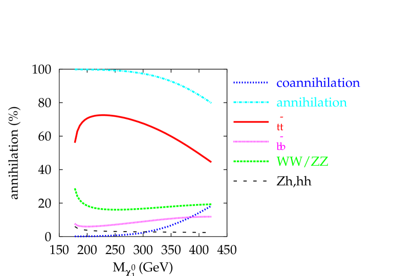
Figure 14: Contribution of the various channels in the focus region. “Annihilation” stands for all the channels which we give individually as $t\bar{t},b\bar{b},W^{+}W^{-},ZZ,Zh$ and $hh$. “Co-annihilation”stands for $\tilde{\chi}_{1}^{0}\tilde{\chi}_{2}^{0},\tilde{\chi}_{1}^{0}\tilde{\chi}_{3}^{0},\tilde{\chi}_{1}^{0}\chi_{1}^{\pm}$.

The contribution of the most important channels to the relic density along slope S3 are displayed in Fig. 14. First of all, note that in our scenario annihilation into tops is always the largest contribution. This comes about through the Goldstone component of $Z$ exchange, which picks up the large top Yukawa coupling. Because of the relatively large Higgsino component, the neutral Goldstone boson couples like $M_{Z}M_{1}/(M_{1}^{2}-\mu^{2})$, with $\mu$ not much larger than $M_{1}$. We also note that we get a non negligible contribution from annihilation into $b\bar{b}$. This contribution is due to $A$ exchange which, contrary to the $t\bar{t}$ contribution via $Z$ exchange, gets a large $\tan\beta$ enhancement. Properties of this contribution are similar to those in the funnel region, though here it is diluted by comparison because of the much larger pseudo-scalar masses involved and also because we are far away from the pole. Although the $\tilde{\chi}_{1}^{0}\tilde{\chi}_{1}^{0}A$ coupling is slightly larger than the $\tilde{\chi}_{1}^{0}\tilde{\chi}_{1}^{0}Z$ coupling, there is a factor of $\mu/M_{1}$ between the two couplings, annihilation through $A$ exchange is suppressed by the large mass of the Higgs in the propagator, compared to the mass of the $Z$ for the $t\bar{t}$ channel. Note the other annihilation channels into $WW,ZZ,Zh,hh$ which account for $10\%$. For LSP masses around $350$GeV, co-annihilation with the heavier neutralino starts to contribute since the $M_{1},\mu$ mass difference gets smaller. From these observations, the fact that quite a few channels and mechanisms are contributing and that the masses involved are quite high will make a precise probe of this scenario rather difficult for the colliders.

6.2 Theoretical uncertainties

Theoretically, the focus point regime is also fraught with difficulties. The position of the focus point region is extremely sensitive to the value of the $\overline{DR}$ MSSM top Yukawa coupling $h_{t}$ [63, 30], which differs for different RGE codes [50]. $h_{t}$ is fixed by the MSSM value of the running top quark mass. In order to obtain this, supersymmetric and Standard Model corrections are subtracted from the top pole mass [49]. The way in which this is done differs in terms which are formally of higher order in the various codes. For example, some codes use pole masses for particles in the loops whereas some use running masses. The radiative corrections are sometimes calculated at different scales. For the case of SOFTSUSY, values of the top quark mass lower than the present 1$\sigma$ range are necessary to reach the region where the relic density is in agreement with the WMAP constraint if $\tan\beta$ is intermediate (e.g. 10-30). This is the reason we concentrated on a high $\tan\beta=50$. We have checked that the numerical results are similar (along a different slope consistent with the WMAP measurement) for $\tan\beta=10$ and $m_{t}=172$ GeV.

Figure 15: (a)$\Omega h^{2}$ along slope S3. The central line gives the default SOFTSUSY prediction, with the broken lines representing the limits due to scale uncertainty. The range of the abscissa corresponds to $M_{1/2}=440-1000$GeV. (b)Relic density dependence upon different approximations in SOFTSUSY for $M_{1/2}=495$GeV, $A_{0}=0$, $\tan\beta=50$ and $\mu>0$. The curves refer to the following approximations: (full calculation): the default full calculation, (2 loop QCD): the default calculation with the 2-loop QCD corrections removed from the extraction of ${m_{t}}^{\overline{DR}}_{MSSM}(m_{t})$, (EW/Higgs): the default calculation with the one-loop electroweak and Higgs corrections removed from the extraction of ${m_{t}}^{\overline{DR}}_{MSSM}(m_{t})$, (neutralinos): the default calculation with the one-loop neutralino corrections removed from the extraction of ${m_{t}}^{\overline{DR}}_{MSSM}(m_{t})$, (charginos): the default calculation with the one-loop chargino corrections removed from the extraction of ${m_{t}}^{\overline{DR}}_{MSSM}(m_{t})$, (2-loops Higgs RGE): the default calculation with only 1-loop RGEs for the Higgs potential soft SUSY breaking parameters $m_{H_{1}}^{2}$, $m_{H_{2}}^{2}$, $m_{3}^{2}$, the 2-loops Higgs RGE are thus removed. (non-resummed $m_{b}$): the default calculation with no re-summation in SUSY $m_{b}$ corrections.

It can be seen from Fig. 15(a) that the prediction of the relic density for the default SOFTSUSY prediction (the unbroken line) is consistent with the WMAP measurement along S3 between $M_{1/2}=440-1000$ GeV (corresponding to $m_{0}=4185-5611$ GeV). However, when $M_{SUSY}$ is varied by a factor of 2 in each direction, the prediction can increase by up to 20$\%$ and decrease by up to 30$\%$. This illustrates that the theoretical uncertainties are large for the focus point regime.

We now examine the theoretical uncertainty on the predictions in more detail. We use various approximations when calculating the sparticle mass spectrum and plot different values predicted for $\Omega h^{2}$ as a function of $m_{0}$, for $M_{1/2}=495$GeV, $A_{0}=0$, $\tan\beta=50$, $\mu>0$. We are therefore moving away from slope S3 to show that different approximations do lead to different parameterisations. The results are displayed in Fig. 15(b). We can see the extreme sensitivity to loop effects from the vastly different values of $m_{0}$ that agree with the WMAP constraints from the figure. The Higgs mass parameter RG evolution becomes very steep near $M_{SUSY}$, and so the sensitivity to the number of loops used to evolve is high. The high sensitivity to the extracted value of $h_{t}$ is shown by the high sensitivity to the approximations in the calculation of ${m_{t}}^{\overline{DR}}_{MSSM}(m_{t})$. At high $\tan\beta=50$, $h_{b}$, the bottom Yukawa coupling is large and affects the running of $m_{H_{1}}^{2}$ appreciably. Its extraction, as we have seen in the previous section, requires knowledge of $\Delta m_{b}$. There was no visible difference from the default calculation by using only one loop running for the gaugino masses $M_{1,2,3}$ instead of the default two-loop running, or removing all 2-loop terms while calculating the Higgs masses and electroweak symmetry breaking conditions.

6.3 Accuracies in mSUGRA

Figure 16: Fractional accuracy required to achieve WMAP precision in the mSUGRA scenario along slope S3: (a) Standard Model inputs, (b) mSUGRA inputs. The range of the abscissa corresponds to $M_{1/2}=440-1000$ GeV.

We now turn to the issue of sensitivity of the $\Omega h^{2}$ prediction to the inputs in the focus point region. As explained in section 2, we imagine that fits to LHC data have identified the mSUGRA SUSY breaking parameters. This would then allow one to derive the entire set of the weak scale parameters, in particular all of those which are of relevance for the calculation of the relic density. As usual it is not only the mSUGRA SUSY parameters at high scales which are needed but also the SM input parameters. Considering what we have just seen concerning the crucial role played by the top Yukawa coupling both in the RGE and in the $t\bar{t}$ annihilation, we expect that a very precise input top pole mass is required as well as $\alpha_{s}(M_{Z})$, one of the parameters that strongly affects the extraction of ${h_{t}}^{\overline{DR}}_{MSSM}$ from $m_{t}$. Fig. 16a shows that there is indeed a huge sensitivity to $m_{t}$ and even $\alpha_{s}(M_{Z})$. $a(m_{b}(m_{b}))\sim\mathcal{O}(1-15)\%$ is shown as an insert in the figure. Values of $a(m_{t})\sim 10^{-4}$ mean that empirical uncertainties of around 20 MeV on $m_{t}$ would be required for WMAP precision. Studies suggest that $\delta(m_{t})\sim 30$ MeV is possible for the statistical error [27] at a suitable linear collider, but that theoretical errors of order $100$MeV are likely. $\alpha_{s}(M_{Z})^{\overline{MS}}_{SM}$ must be measured to better than an order of magnitude more precisely than current data allow.

Fig. 16b shows that $m_{0}$ must be measured to a fractional precision of better than $0.2\%$ for WMAP accuracy. Such an accuracy is inconceivable at the LHC because, among other reasons, the production cross-sections for the multi-TeV scalars present in the focus-point region are tiny. In mSUGRA, $m_{0}$ determines (among others things) the value of $\mu$ which determines the amount of Higgsino content. $M_{1/2}$ also affects the determination of $\mu$ as well as the mass of the LSP. We find that $M_{1/2}$ should be measured to better than $0.5\%$ for WMAP accuracy, and $A_{0}$ to better than 180 GeV, provided $m_{t}$ is not quasi-degenerate with $M_{\tilde{\chi}_{1}^{0}}$. The sudden deterioration in the accuracy for $M_{\tilde{\chi}_{1}^{0}}\sim m_{t}$ is due to the approach to the $t$ threshold. A similar behaviour is seen in the required accuracy of $\tan\beta$. The measurement of $\tan\beta$ in mSUGRA will be very demanding, due not only to the importance of the $t\bar{t}$ vertex but also the extraction of the top Yukawa that enters the RGE.

6.4 Accuracies in PmSUGRA

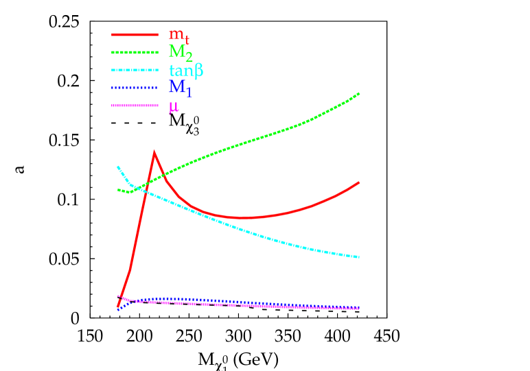
Figure 17: Required fractional accuracy upon MSSM parameters in the PmSUGRA scenario along slope S3. The abscissas correspond to $M_{1/2}=440-1000$ GeV.

Fig. 17 displays the required accuracies $a$ for several parameters in the PmSUGRA scenario. The relevant parameters are the weak scale values of the elements of the neutralino mass matrix. In particular, $M_{1}$ and $\mu$ are important since, as discussed already, they determine the Higgsino component of the LSP and how large the couplings of the LSP to the Higgs bosons, $W$ and $Z$ are. $\tan\beta$ enters in the contribution of the $b\bar{b}$ annihilation and in the neutralino couplings. Since $M_{2}$ is not completely decoupled its effect is expected to feed in as well. All of these parameters are essential for the co-annihilation processes that set in for higher LSP masses. Finally, there is also dependence upon $M_{A}$. Before we discuss these accuracies and in order to highlight the contrast with the mSUGRA approach, we comment on the accuracy needed on $m_{t}$. $m_{t}$ enters through the coupling of the neutral Goldstone boson as $m_{t}^{2}$ (taking the dominant contribution) when the top threshold sets in. We find a sensitivity to $m_{t}$ which is typically of the same order as the precision on the relic density. The present empirical precision on $m_{t}$ is sufficient even for the PLANCK benchmark. At the top threshold one requires a much better accuracy. On the other hand, the accuracy is less demanding for higher LSP masses since the contribution of the $t\bar{t}$ annihilation is smaller. A rough estimate on $a(m_{t})$, away from threshold, is $a(m_{t})\sim 1/(2c_{t})$ in units of the precision on the relic and where $c_{t}$ is the relative contribution of the $t\bar{t}$ channel. $c_{t}$ can be read off from Fig. 14. Similarly in the whole range of $M_{1/2}$ considered, $a(m_{b})>3.0$ meaning that even the present empitical $m_{b}$ errors reach PLANCK accuracy. The sensitivities of $\mu,M_{1}$ require fractional precisions of 1$\%$ for WMAP accuracy. This rather demanding accuracy originates more from the couplings of the LSP to the Goldstone and $A$ pseudo-scalar bosons. As we show in the figure, the accuracies on $M_{1}$ and $\mu$ can be converted into accuracies on $m_{\tilde{\chi}_{1}^{0}}$ and $m_{\tilde{\chi}_{3}^{0}}$. The accuracy needed on $M_{2}$ is an order of magnitude worse, though it is still non trivial to obtain empirically. Therefore we see that if one can reconstruct the neutralino mass matrix, which we think can be done rather precisely at the LC provided there is enough energy to produce all of the neutralinos, this scenario can be very much constrained. It could be interesting to study whether this could be done without direct production of the heaviest (wino-like) neutralino and how a combination of LHC and LC data could be performed. A slight problem still remains as concerns the $M_{A}$ dependence and its required accuracy. In this scenario $M_{A}$ is very large, in excess of $1$TeV and could be difficult to access at the LHC or a sub-TeV LC. We find that at the lower end of the focus region, a change of $50\%$ or higher in $M_{A}$ only amounts to a maximum $5\%$ change in the relic density. However, at the higher end, though $M_{A}\sim 1.5TeV$, a $30\%$ change in $M_{A}$ affects the relic density by $10\%$. The reason that a larger (positive) change does not deteriorate the precision is due to the propagator suppression of $M_{A}$ which means that the $A$ exchange no longer contributes for too high values of $M_{A}$.

7 Summary and Conclusions

Assuming mSUGRA, we have examined the requirements for measurements of the MSSM spectrum in order to make reliable predictions of the relic density $\Omega h^{2}$. If such requirements could be met, the assumptions that go into the derivation of $\Omega h^{2}$ may be tested.

We find that theoretical uncertainties in the mSUGRA prediction of $\Omega h^{2}$ assuming standard cosmology are too high compared with the WMAP prediction. In the co-annihilation scenario, the theoretical uncertainty in $\Omega h^{2}$ (estimated by scale dependence) is of the same size to twice as big as the WMAP accuracy. The situation is worse in the problematic focus point and higher mass Higgs funnel regions, where the theory scale variation is around five times bigger than the WMAP accuracy. In the lighter Higgs funnel region, the scale variation is smaller than the WMAP accuracy. The theoretical uncertainties are not a serious problem, since higher order calculations should be possible given enough time, effort and motivation. If SUSY particles are discovered at a future collider, it seems highly likely that this task will be accomplished.

The experimental information necessary in order to achieve a precise prediction of the relic density is demanding. If one assumes mSUGRA, fits must constrain $M_{1/2}$ and $m_{0}$ at the one or two percent level and $A_{0}$ to roughly 100 GeV, for the co-annihilation region for example. It is estimated in a bulk-region test case [14] that at the LHC this accuracy is not quite achievable, even when the parameters are quite favourable (for example $m_{0}=103\pm 8$ GeV, $M_{1/2}=240.0\pm 3$ GeV at post-WMAP benchmark point B), but is an order of magnitude too large at other points ($m_{0}=400\pm 100$ GeV and $M_{1/2}=400\pm 8$ GeV at LHC points 1,2 [53]). Combining complementary information from the LHC and a future linear collider should provide the necessary precision, however [64, 65, 66]. Not only must one experimentally control the soft SUSY breaking parameters assuming mSUGRA, but Standard Model inputs must also be controlled if the calculation of the MSSM spectrum is to be trusted. In the co-annihilation region this is not a big problem, since the parts of the spectrum relevant to the prediction of $\Omega h^{2}$ (the lightest neutralino and stau) do not have a large sensitivity to the Standard Model inputs. The sensitivity in the focus point region to the top Yukawa coupling $h_{t}$ is so high that $m_{t}$ must be measured to better than 20 MeV. This is smaller than the strong scale of the QCD interaction and therefore cannot be perturbatively defined with such precision, rendering the approach practically hopeless. In the Higgs funnel region, $m_{t}$ must be measured to around 200 MeV, which may be achieved at a future linear collider facility, but $m_{b}(m_{b})$ must be constrained to the 2-10 per mille level because of its effect on the mass of the pseudo-scalar Higgs, which participates in the $s$-channel to neutralino annihilation. This will not be possible since it is much smaller than non-perturbative effects, but by measuring the mass of the $A$ at the percent level, the sensitive dependence upon $m_{b}(m_{b})$ can be removed. For the heavier decoupled values of $m_{A}$, a linear collider with sufficient centre of mass energy will be required since the LHC will not provide enough precision on measurements of the $A$ bosons [67].

Rather than relying upon mSUGRA to make predictions for the spectrum, a more general strategy is to first determine what regime one is in. If quasi-degenerate lightest stau and neutralinos are discovered for example, it would indicate a co-annihilation regime. In that case the mass splitting (less than 12 GeV) must be measured to better than $1$GeV in order to achieve WMAP precision upon $\Omega h^{2}$ for LSP and $\tilde{\tau}_{1}$ weighing between $150$ to $450$GeV. In the focus point regime (indicated by the measurement of gauginos but non-observation of scalars at the LHC), the extreme sensitivity to $m_{t}$ vastly reduces if one no longer has to assume mSUGRA and relies on individual mass measurements instead. However, a measurement of $\mu$ and $M_{1}$ to 1$\%$ accuracy is required and will require copious production of neutralinos and charginos at a linear collider with sufficient centre of mass energy [68, 69] since the masses involved are high. In the Higgs funnel scenario, the quantity $2M_{\tilde{\chi}_{1}^{0}}-M_{A}$ must be measured very precisely requiring a measurement of $M_{A}$ and $m_{\tilde{\chi}_{1}^{0}}$ with a precision ranging from $2\%$ for LSP masses around $100$GeV to $0.2\%$ for LSP masses around $450$GeV.

The analysis we have performed in this paper was done in the mSUGRA framework. WMAP now allows only three scenarios in mSUGRA which are quite contrived and are challenging both from the theoretical and experimental point of view. Going beyond mSUGRA, for example in a scenario with non universal gaugino masses and in particular a wino-like LSP, would be subject to less theory uncertainty and might call for accuracies that are less demanding for the colliders. It is also important to stress that we have assumed that the standard derivation of the relic density is correct. However, one should not forget that most alternatives that affect the cosmological assumptions usually predict orders of magnitude differences with the orthodox approach, far beyond the few percent precision we have taken as a benchmark. This means that perhaps some of these alternatives could be dismissed without requiring too much precision. On the other hand it would be interesting, assuming such schemes to be correct, to inquire about the level of accuracy on the particle physics parameters that the colliders must meet to corroborate some of these non-standard cosmologies.

Appendix A Inputs

Except where explicitly mentioned, we use the following default Standard Model parameters as inputs [70]:

$$\alpha_{s}(M_{Z})^{\overline{MS}}_{SM} = 0.1172,\ \alpha(M_{Z})^{\overline{MS}}_{SM}=1/(127.934),\ m_{b}(m_{b})^{\overline{MS}}=4.23\mbox{~{}GeV},$$

$$m_{\tilde{\tau}} = 1.7777\mbox{~{}GeV},\ M_{Z}=91.1876~{}\mbox{~{}GeV},\ m_{t}=175\mbox{~{}GeV}.$$ (24)

A subscript $SM$ denotes the fact that the quantity has been derived assuming Standard Model field content. $m_{b}(m_{b})^{\overline{MS}}$ is derived from experiment in 5-flavour QCD. A $\overline{MS}$ superscript denotes a quantity calculated in the modified minimal subscription renormalisation scheme. The weak mixing angle is derived from the muon decay constant $G_{\mu}=1.16637\times 10^{-5}$ GeV^-2.

The mSUGRA parameters are specified as $\tan\beta$, the ratio of the two Higgs vacuum expectation values, the universal gaugino mass $M_{1/2}$, the universal trilinear scalar coupling $A_{0}$ and the universal scalar mass $m_{0}$. Universality is imposed upon the soft SUSY breaking terms at a scale $M_{GUT}$ which is defined by

$$g_{1}(M_{GUT})=g_{2}(M_{GUT}),$$ (25)

$g_{1}$ and $g_{2}$ being the electroweak gauge couplings in the modified $\overline{DR}$ scheme. $g_{1}$ is related to the Standard Model hypercharge coupling $g^{\prime}$ by the GUT normalisation $g_{1}=\sqrt{5/3}g^{\prime}$. $g_{3}$ is set by the $\alpha_{s}(M_{Z})^{\overline{MS}}_{SM}$ input and is not unified with $g_{1,2}$. We will take the Higgs potential parameter $\mu>0$, with its magnitude being fixed by the electroweak symmetry breaking conditions [32].

References

- [1] J. R. Ellis, J. S. Hagelin, D. V. Nanopoulos, K. A. Olive, and M. Srednicki, Supersymmetric relics from the big bang, Nucl. Phys. B238 (1984) 453–476.
- [2] E. W. Kolb and M. S. Turner, The early universe, . Redwood City, USA: Addison-Wesley (1990) 547 p. (Frontiers in physics, 69).
- [3] H. Baer and C. Balazs, analysis of the minimal supergravity model including wmap, g(mu)-2 and b s gamma constraints, JCAP 0305 (2003) 006, [hep-ph/0303114].
- [4] J. R. Ellis, K. A. Olive, Y. Santoso, and V. C. Spanos, Supersymmetric dark matter in light of wmap, Phys. Lett. B565 (2003) 176–182, [hep-ph/0303043].
- [5] U. Chattopadhyay, A. Corsetti, and P. Nath, Wmap constraints, susy dark matter and implications for the direct detection of susy, Phys. Rev. D68 (2003) 035005, [hep-ph/0303201].
- [6] A. B. Lahanas and D. V. Nanopoulos, Wmaping out supersymmetric dark matter and phenomenology, Phys. Lett. B568 (2003) 55–62, [hep-ph/0303130].
- [7] D. N. Spergel et. al., First year wilkinson microwave anisotropy probe (wmap) observations: Determination of cosmological parameters, Astrophys. J. Suppl. 148 (2003) 175, [astro-ph/0302209].
- [8] C. L. Bennett et. al., First year wilkinson microwave anisotropy probe (wmap) observations: Preliminary maps and basic results, Astrophys. J. Suppl. 148 (2003) 1, [astro-ph/0302207].
- [9] J. Lesgourgues, S. Prunet, and D. Polarski, Parameters extraction by planck for a cdm model with bsi steplike primordial spectrum and cosmological constant, Mon. Not. Roy. Astron. Soc. 303 (1999) 45–49, [astro-ph/9807020].
- [10] A. Balbi, C. Baccigalupi, F. Perrotta, S. Matarrese, and N. Vittorio, Probing dark energy with the cmb: projected constraints from map and planck, Astrophys. J. 588 (2003) L5–L8, [astro-ph/0301192].
- [11] H. Baer et. al., Updated constraints on the minimal supergravity model, JHEP 07 (2002) 050, [hep-ph/0205325].
- [12] G. Bélanger, F. Boudjema, A. Cottrant, A. Pukhov, and A. Semenov, Wmap constraints on sugra models with non-universal gaugino masses and prospects for direct detection, hep-ph/0407218.
- [13] E. A. Baltz and P. Gondolo, Markov chain monte carlo exploration of minimal supergravity with implications for dark matter, hep-ph/0407039.
- [14] M. Battaglia et. al., Updated post-wmap benchmarks for supersymmetry, Eur. Phys. J. C33 (2004) 273–296, [hep-ph/0306219].
- [15] G. F. Giudice, E. W. Kolb, and A. Riotto, Largest temperature of the radiation era and its cosmological implications, Phys. Rev. D64 (2001) 023508, [hep-ph/0005123].
- [16] S. Khalil, C. Munoz, and E. Torrente-Lujan, Relic neutralino density in scenarios with intermediate unification scale, New J. Phys. 4 (2002) 27, [hep-ph/0202139].
- [17] P. Salati, Quintessence and the relic density of neutralinos, Phys. Lett. B571 (2003) 121–131, [astro-ph/0207396].
- [18] F. Rosati, Quintessential enhancement of dark matter abundance, Phys. Lett. B570 (2003) 5–10, [hep-ph/0302159].
- [19] M. Joyce, On the expansion rate of the universe at the electroweak scale, Phys. Rev. D55 (1997) 1875–1878, [hep-ph/9606223].
- [20] M. Joyce and T. Prokopec, Baryogenesis from ’electrogenesis’ in a scalar field dominated epoch, JHEP 10 (2000) 030, [hep-ph/0003190].
- [21] T. Nihei, N. Okada, and O. Seto, Neutralino dark matter in brane world cosmology, hep-ph/0409219.
- [22] M. Kamionkowski and M. S. Turner, Thermal relics: Do we know their abundances?, Phys. Rev. D42 (1990) 3310–3320.
- [23] S. Profumo and P. Ullio, Neutralino relic density enhancement in non-standard cosmologies, astro-ph/0404390.
- [24] R. Catena, N. Fornengo, A. Masiero, M. Pietroni, and F. Rosati, Dark matter relic abundance and scalar-tensor dark energy, astro-ph/0403614.
- [25] B. Murakami and J. D. Wells, Nucleon scattering with higgsino and wino cold dark matter, Phys. Rev. D64 (2001) 015001, [hep-ph/0011082].
- [26] ATLAS and CMS Collaboration, J. G. Branson et. al., High transverse momentum physics at the large hadron collider: The atlas and cms collaborations, Eur. Phys. J. direct C4 (2002) N1.
- [27] ECFA/DESY LC Physics Working Group Collaboration, J. A. Aguilar-Saavedra et. al., Tesla technical design report part iii: Physics at an e+e- linear collider, hep-ph/0106315.
- [28] B. C. Allanach, D. Grellscheid, and F. Quevedo, Selecting supersymmetric string scenarios from sparticle spectra, JHEP 05 (2002) 048, [hep-ph/0111057].
- [29] B. C. Allanach, D. Grellscheid, and F. Quevedo, Genetic algorithms and experimental discrimination of susy models, hep-ph/0406277.
- [30] B. C. Allanach, S. Kraml, and W. Porod, Theoretical uncertainties in sparticle mass predictions from computational tools, JHEP 03 (2003) 016, [hep-ph/0302102].
- [31] B. C. Allanach, A. Djouadi, J. L. Kneur, W. Porod, and P. Slavich, Precise determination of the neutral higgs boson masses in the mssm, hep-ph/0406166.
- [32] B. C. Allanach, Softsusy: A c++ program for calculating supersymmetric spectra, Comput. Phys. Commun. 143 (2002) 305–331, [hep-ph/0104145].
- [33] G. Bélanger, F. Boudjema, A. Pukhov, and A. Semenov, Micromegas: Version 1.3, hep-ph/0405253.
- [34] P. Skands et. al., Susy les houches accord: Interfacing susy spectrum calculators, decay packages, and event generators, hep-ph/0311123.
- [35] F. Boudjema, Physics for the future colliders, hep-ph/0105040.
- [36] M. Brhlik, D. J. H. Chung, and G. L. Kane, Weighing the universe with accelerators and detectors, Int. J. Mod. Phys. D10 (2001) 367, [hep-ph/0005158].
- [37] M. Drees et. al., Scrutinizing lsp dark matter at the lhc, Phys. Rev. D63 (2001) 035008, [hep-ph/0007202].
- [38] G. Polesello and D. R. Tovey, Constraining susy dark matter with the atlas detector at the lhc, JHEP 05 (2004) 071, [hep-ph/0403047].
- [39] P. Bambade, M. Berggren, F. Richard, and Z. Zhang, Experimental implications for a linear collider of the susy dark matter scenario, hep-ph/0406010.
- [40] H.-U. Martyn, Detection of sleptons at a linear collider in models with small slepton neutralino mass differences, hep-ph/0408226.
- [41] B. C. Allanach et. al., The snowmass points and slopes: Benchmarks for susy searches, Eur. Phys. J. C25 (2002) 113–123, [hep-ph/0202233].
- [42] K. Griest and D. Seckel, Three exceptions in the calculation of relic abundances, Phys. Rev. D43 (1991) 3191–3203.
- [43] M. Drees and M. M. Nojiri, The neutralino relic density in minimal n=1 supergravity, Phys. Rev. D47 (1993) 376–408, [hep-ph/9207234].
- [44] R. Arnowitt and P. Nath, Cosmological constraints and su(5) supergravity grand unification, Phys. Lett. B299 (1993) 58–63, [hep-ph/9302317].
- [45] J. L. Feng, K. T. Matchev, and T. Moroi, Focus points and naturalness in supersymmetry, Phys. Rev. D61 (2000) 075005, [hep-ph/9909334].
- [46] J. L. Feng, K. T. Matchev, and F. Wilczek, Neutralino dark matter in focus point supersymmetry, Phys. Lett. B482 (2000) 388–399, [hep-ph/0004043].
- [47] A. Birkedal-Hansen and E.-h. Jeong, Gaugino and higgsino coannihilations. i: Neutralino neutralino interactions, JHEP 02 (2003) 047, [hep-ph/0210041].
- [48] H. Baer, C. Balazs, and A. Belyaev, Neutralino relic density in minimal supergravity with co- annihilations, JHEP 03 (2002) 042, [hep-ph/0202076].
- [49] D. M. Pierce, J. A. Bagger, K. T. Matchev, and R.-j. Zhang, Precision corrections in the minimal supersymmetric standard model, Nucl. Phys. B491 (1997) 3–67, [hep-ph/9606211].
- [50] B. C. Allanach, G. Bélanger, F. Boudjema, A. Pukhov, and W. Porod, Uncertainties in relic density calculations in msugra, hep-ph/0402161.
- [51] S.P. Martin, Two-loop effective potential for the minimal supersymmetric standard model, Phys. Rev. D66 (2002) 096001, hep-ph/0206136.
- [52] S.P. Martin, Strong and Yukawa two-loop contributions to Higgs scalar boson self-energies and pole masses in supersymmetry, hep-ph/0405022.
- [53] ATLAS Collaboration, W. W. Armstrong et. al., Atlas: Technical proposal for a general-purpose p p experiment at the large hadron collider at cern, . CERN-LHCC-94-43.
- [54] M. E. Gomez, T. Ibrahim, P. Nath, and S. Skadhauge, Sensitivity of supersymmetric dark matter to the b quark mass, hep-ph/0404025.
- [55] G. Bélanger, F. Boudjema, A. Pukhov, and A. Semenov, micromegas: A program for calculating the relic density in the mssm, Comput. Phys. Commun. 149 (2002) 103–120, [hep-ph/0112278].
- [56] M. M. Nojiri, K. Fujii, and T. Tsukamoto, Confronting the minimal supersymmetric standard model with the study of scalar leptons at future linear e+ e- colliders, Phys. Rev. D54 (1996) 6756–6776, [hep-ph/9606370].
- [57] R. Arnowitt, B. Dutta, T. Kamon, and V. Khotilovich, msugra at a 500-gev linear collider, hep-ph/0308159.
- [58] I. Jack, D. R. T. Jones, and A. F. Kord, Snowmass benchmark points and three-loop running, hep-ph/0408128.
- [59] E. Boos et. al., Polarisation in sfermion decays: Determining tan(beta) and trilinear couplings, Eur. Phys. J. C30 (2003) 395–407, [hep-ph/0303110].
- [60] K. Griest and D. Seckel, Three exceptions in the calculation of relic abundances, Phys. Rev. D43 (1991) 3191–3203.
- [61] M. Carena, H. E. Haber, H. E. Logan, and S. Mrenna, Distinguishing a mssm higgs boson from the sm higgs boson at a linear collider, Phys. Rev. D65 (2002) 055005, [hep-ph/0106116].
- [62] J. L. Feng, K. T. Matchev, and T. Moroi, Multi-tev scalars are natural in minimal supergravity, Phys. Rev. Lett. 84 (2000) 2322–2325, [hep-ph/9908309].
- [63] B. C. Allanach, J. P. J. Hetherington, M. A. Parker, and B. R. Webber, Naturalness reach of the large hadron collider in minimal supergravity, JHEP 08 (2000) 017, [hep-ph/0005186].
- [64] G. A. Blair, W. Porod, and P. M. Zerwas, Reconstructing supersymmetric theories at high energy scales, Phys. Rev. D63 (2001) 017703, [hep-ph/0007107].
- [65] G. A. Blair, W. Porod, and P. M. Zerwas, The reconstruction of supersymmetric theories at high energy scales, Eur. Phys. J. C27 (2003) 263–281, [hep-ph/0210058].
- [66] B. C. Allanach et. al., Reconstructing supersymmetric theories by coherent lhc / lc analyses, hep-ph/0403133.
- [67] M. Battaglia, Cold dark matter inspire cmssm scenarios at a 1 tev linear collider, . Can be found at URL http://www.linearcollider.ca:8080/lc/vic04/abstracts/physics/cosmology/.
- [68] S. Y. Choi, J. Kalinowski, G. Moortgat-Pick, and P. M. Zerwas, Analysis of the neutralino system in supersymmetric theories, Eur. Phys. J. C22 (2001) 563–579, [hep-ph/0108117].
- [69] S. Y. Choi et. al., Reconstructing the chargino system at e+ e- linear colliders, Eur. Phys. J. C14 (2000) 535–546, [hep-ph/0002033].
- [70] K. Hagiwara et. al., Review of Particle Physics, Phys. Rev. D 66 (2002) 010001.