Electroweak supersymmetric effects on high energy unpolarized and polarized single top production at LHC.

Abstract

We consider various processes of single top production at LHC in the theoretical framework of the MSSM and examine the role of the supersymmetric electroweak one-loop corrections in a special moderately light SUSY scenario, in an initial parton-pair c.m. high energy range where a logarithmic asymptotic expansion of Sudakov type can be used. We show that the electroweak virtual effects are systematically large, definitely beyond the relative ten percent size, particularly for a final $tH^{-}$ pair where a special enhancement is present. We show then in a qualitative way the kind of precision tests of the model that would be obtainable from accurate measurements of the energy distributions of the various cross sections and of the top polarization asymmetries.

I Introduction

The process of single top production in proton-proton collisions has recently been described in detail [1] and its relevance in theoretical models of electroweak physics has been stressed with special emphasis. In the particular framework of the Standard Model, the relevant final pairs can be (at partonic level): 1) a top and a light quark ($t$-channel production), 2) a top and a $\bar{b}$ ($s$-channel production), 3) a top and a $W^{-}$ (associated production), and the corresponding Feynman diagrams at Born level are shown in Fig.1,2. As stressed in Ref.[1], from precise measurements of these processes the first direct determination of the CKM $Wtb$ coupling at hadron colliders will be obtained, which already motivates the existence of dedicated experimental and theoretical studies.

The theoretical analysis of the first two processes has been performed in a number of papers, both within the SM and beyond it, with special emphasis on the production at TEVATRON [2]. The third process will only be measured at LHC, and to our knowledge a detailed theoretical study at the perturbative one-loop level, valid in particular for the MSSM, does not exist yet.

In this paper, we shall assume a preliminary discovery of supersymmetry at LHC (perhaps already at TEVATRON) and a SUSY scenario of a ”moderately” light kind, in which all sparticle masses lie below, say, approximately three-four hundred GeV. Our aim will be that of showing that, under these conditions, single top production at LHC might provide crucial, accurate precision tests of the candidate theoretical model. For this preliminary analysis we shall stick to the MSSM, but our treatment could be modified in a straightforward way to examine less simple supersymmetric proposals.

In our analysis, we shall consider ”large” values of the initial parton pair c.m. energy $\sqrt{s}$, typically of the 1 TeV size. There exist two main reasons that motivate our choice. The first one is that within this energy range we shall feel entitled to make use, at the one-loop perturbative level, of a simple asymptotic logarithmic expansion of so called Sudakov kind, whose validity in the MSSM is related to the assumption of a light SUSY scenario, so that $s/M^{2}$ (the typical parameter of the logarithmic expansion) is of order ten ($M$ is the heaviest SUSY mass of the scenario). The second one is that, for $\sqrt{s}$ values much larger than the final $t$, $W$ masses, remarkable kinematical simplifications arise whose theoretical origin will be shown. These make, in particular, the treatment of the associated production process much simpler, and allow to understand the potentialities of its relevant supersymmetric effect from inspection of short analytic formulae.

The plan of this paper will be the following. In Section 2A we shall briefly derive the expressions of the electroweak Sudakov expansions at one loop to next-to leading order, i.e. retaining the squared and the linear logarithmic terms, for the $t$- and $s$-channel processes. For the latter, a partial MSSM calculation of the Yukawa effect is already available, in an arbitrary c.m. energy configuration where in general all the parameters of the model will enter the theoretical predictions [3]; our calculation will include logarithmic terms of several origins, but owing to our energy choice a strongly reduced number of parameters will remain in the relevant expressions, as we shall show in detail. Section 2B will be devoted to a more accurate description of the determination of the Sudakov expansion for the so called associated $tW$ production process. Here, as we said, a theoretical calculation in the MSSM is not known to us; independently of this, we shall comment anyway a few special features of our expansions, in particular the simplifications due to the choice of a high energy regime. Within the MSSM, another process to be added to the previously considered ones seems to us to be that of $tH^{-}$ production. This has also been already studied in an arbitrary energy configuration [4],[5],[6]; we shall derive here in Section 2C only its electroweak logarithmic Sudakov expansion, to be compared with the three previous ones to have a more complete description of the asymptotic single top production at LHC.

A final topic that seems to us to deserve some consideration is that of the single top polarization. This is automatically fixed in the $t$, $s$ channel processes in the chosen high energy region where the final top must be of left-handed type; this feature is not valid for $tW^{-}$ and $tH^{-}$ production. As a consequence, one may in principle consider longitudinal polarization asymmetries for these processes. In Section 2D, we shall derive the asymptotic expressions of these quantities, that will turn out to be relatively simple.

Having at disposal all the relevant asymptotic expressions for the four considered processes, we shall then devote Section 3 to an investigation of which kind of precision test of the model could be provided by realistic experimental measurements. This will be done in a necessarily qualitative way, exploiting the available preliminary conclusions of Ref.[1], assuming that the distributions in $\sqrt{s}$ can be determined with a certain accuracy in our chosen range. Our presentation will remain for the moment at a qualitative level. In fact, the purpose of our paper is mostly that of showing the possible relevance of measurements that appear to us, at least in principle, performable, and to encourage an experimental performance like that indicated in Ref.[1]. This point will be discussed in the final conclusions, given in the short Section 4.

II Single top production

As we said, this Section will be devoted to a derivation of the asymptotic electroweak expressions for the four considered processes. To save space and time, since the major part of the relevant technical definitions and properties has been already exhaustively illustrated in previous papers [7], we shall quickly write the final formulae for the ($t,d$), ($t,\bar{b}$) and ($t,H^{-}$) processes, that have already been studied in the literature (but not in our chosen scenario) as we anticipated. The treatment of the final ($t,W^{-}$) pair will be slightly more detailed since for this process, as we said, we are not aware of a theoretical investigation in the MSSM, and also since in this case the benefits of the chosen high energy configuration deserve, in our opinion, a short mention.

A T,S CHANNELS SINGLE TOP PRODUCTION

1 $bu\to td$ with $W$ exchange in the $t$ channel

We begin with the $t$-channel process represented in Fig.1a at Born level. As one sees, there is only one diagram with W exchange in the $t$-channel, $t=(p_{b}-p_{t})^{2}$. The corresponding scattering amplitude is:

$$A^{Born}={2\pi\alpha\over s^{2}_{W}(t-m^{2}_{W})}[\bar{u}(d,\tau^{\prime})\gamma^{\mu}P_{L}u(u,\lambda^{\prime})][\bar{u}(t,\tau)\gamma_{\mu}P_{L}u(b,\lambda)]$$ (1)

where $\lambda,\lambda^{\prime},\tau,\tau^{\prime}$ are the $b,u,t,d$ helicities, $P_{R,L}=(1\pm\gamma^{5})/2$ are the projectors on $R,L$ chiralities ans $s_{W}$ is the sine of the Weinberg angle.

It is convenient to work with helicity amplitudes $F_{\lambda,\lambda^{\prime},\tau,\tau^{\prime}}$; retaining only the top mass and setting all the remaining masses equal to zero leaves one single amplitude $F_{----}$:

$$F^{Born}_{----}={4\pi\alpha s\sqrt{\beta}\over s^{2}_{W}(t-m^{2}_{W})}$$ (2)

with $\beta={p_{t}\over E_{t}}=1-{m^{2}_{t}\over s}$.

The expression of the differential cross section is:

$${d\sigma\over dcos\theta}={\beta\over 1152\pi s}\sum_{spin,col}|F_{\lambda\lambda^{\prime}\tau\tau^{\prime}}|^{2}$$ (3)

which becomes after color average:

$${d\sigma^{Born}\over d\cos\theta}={\beta^{2}\pi\alpha^{2}s\over 8s^{4}_{W}(t-m^{2}_{W})^{2}}$$ (4)

At one-loop, the Sudakov electroweak corrections can be of universal and of angular dependent kind, and we follow the definitions of  [7].

The effect of the universal terms on the helicity amplitude can be summarized as follows:

$$F^{Univ}_{----}=F^{Born}_{----}~{}{1\over 2}~{}[~{}c^{ew}(b\bar{b})_{L}+c^{ew}(u\bar{u})_{L}+c^{ew}(d\bar{d})_{L}+c^{ew}(t\bar{t})_{L}]$$ (5)

where:

$$c^{ew}(q\bar{q})_{L}=c^{ew}(\tilde{q}\tilde{\bar{q}})_{L}=c(q\bar{q},~{}gauge)_{L}~{}+~{}c(q\bar{q},~{}yuk)_{L}$$ (6)

$$c(d\bar{d},~{}gauge)_{L}=c(u\bar{u},~{}gauge)_{L}={\alpha(1+26c^{2}_{W})\over 144\pi s^{2}_{W}c^{2}_{W}}~{}(2~{}\log{s\over m^{2}_{W}}-\log^{2}{s\over m^{2}_{W}})$$ (7)

$$c(b\bar{b},~{}yuk)_{L}=c(t\bar{t},~{}yuk)_{L}=-~{}{\alpha\over 8\pi s^{2}_{W}}~{}[\log{s\over m^{2}_{W}}]~{}[{m^{2}_{t}\over m^{2}_{W}}(1+\cot^{2}\beta)+{m^{2}_{b}\over m^{2}_{W}}(1+\tan^{2}\beta)]$$ (8)

Note that we use $m_{W}$ as a scale for the log term. This is mandatory for the squared log which arises from $W$ loops. For what concerns the single log, as we do not consider ”constant terms” this a matter of choice and we decide to keep $m_{W}$ as a scale for the above terms.

The angular dependent terms have the following expression:

$$F^{ang}_{----}=F^{Born}_{----}[~{}c^{ang}_{----}~{}]$$ (9)

$$c^{ang}_{----} = -~{}{\alpha(1+8c^{2}_{W})\over 18\pi s^{2}_{W}c^{2}_{W}}[\log{-u\over s}][\log{s\over m^{2}_{W}}]$$ (11)

$$-~{}{\alpha(1-10c^{2}_{W})\over 36\pi s^{2}_{W}c^{2}_{W}}[\log{-t\over s}][\log{s\over m^{2}_{W}}]$$

At high energy we have $t\simeq-~{}{s\over 2}(1-\cos\theta)$ and $u\simeq-~{}{s\over 2}(1+\cos\theta)$.

There are also SUSY QCD corrections, only of universal kind. We shall treat them as ”known” terms for what concerns our search of electroweak effects; at one loop, their expression is not difficult to be derived, and reads:

$$F^{Univ~{}SUSYQCD}_{----} = F^{Born}_{----}~{}[-\frac{2\alpha_{s}}{3\pi}\log\frac{s}{M_{\rm SUSY}^{2}}]$$ (12)

In addition to the previous terms of Sudakov type, there are at one-loop ”known” linear logarithms of RG origin, whose expression we quote for completeness:

$$F^{RG}_{----} = -~{}{1\over 4\pi^{2}}[g^{4}\tilde{\beta^{0}}{dF^{Born}_{----}\over dg^{2}}][\log\frac{s}{M_{W}^{2}}]$$ (14)

$$={\alpha^{2}s\sqrt{\beta}\over s^{4}_{W}(t-m^{2}_{W})}[\log\frac{s}{M_{W}^{2}}]$$

using the lowest order Renormalization Group $\beta$ function for the gauge coupling $g=e/s_{W}$: $\tilde{\beta^{0}}=-~{}{1\over 4}$ in MSSM.

2 $u\bar{d}\to t\bar{b}$ with $W$ exchange in the $s$ channel

Neglecting again all quark masses with the exception of $m_{t}$ one finds from the Born diagram of Fig. 1b:

$$A^{Born}={e^{2}\over 2s^{2}_{W}(s-m^{2}_{W})}[\bar{v}(\bar{d},\lambda^{\prime})\gamma^{\mu}P_{L}u(u,\lambda)][\bar{u}(t,\tau)\gamma_{\mu}P_{L}v(\bar{b},\tau^{\prime})]$$ (15)

There are now in principle two helicity amplitudes $F_{\lambda,\lambda^{\prime},\tau,\tau^{\prime}}$:

$$F^{Born}_{-+-+}=-~{}{2\pi\alpha s\sqrt{\beta}(1+\cos\theta)\over s^{2}_{W}(s-m^{2}_{W})}$$ (16)

$$F^{Born}_{-+++}=-~{}{2\pi\alpha m_{t}\sqrt{s}\sqrt{\beta}\sin\theta\over s^{2}_{W}(s-m^{2}_{W})}$$ (17)

where $\beta=1-{m^{2}_{t}\over s}$.

Note that the second amplitude $F^{Born}_{-+++}$ is depressed with respect to the first one by the factor $m_{t}/\sqrt{s}$, so that in our chosen configuration it will be treated with some approximations, neglecting its one loop corrections.

In the differential cross section the two contributions will be:

$${d\sigma\over d\cos\theta}={\beta\over 128\pi s}\sum_{spins}|F_{\lambda,\lambda^{\prime},\tau,\tau^{\prime}}|^{2}$$ (18)

$${d\sigma^{Born}\over d\cos\theta}={\beta^{2}\pi\alpha^{2}s\over 32s^{4}_{W}(s-m^{2}_{W})^{2}}[(1+\cos\theta)^{2}+{m^{2}_{t}\over s}\sin^{2}\theta]$$ (19)

where the first term comes from $F_{-+-+}$ and the second one comes from the “depressed” amplitude $F_{-+++}$ that will be retained in Born approximation. For the relevant amplitude $F_{-+-+}$, we obtain the following effects:

$$F^{Univ}_{-+-+} = F^{Born}_{-+-+}~{}{1\over 2}~{}[~{}c^{ew}(b\bar{b})_{L}+c^{ew}(u\bar{u})_{L}+c^{ew}(d\bar{d})_{L}+c^{ew}(t\bar{t})_{L}]$$ (20)

with the expressions of the various $c_{ew}$ given for the $t$-channel case and

$$F^{ang}_{-+-+} = {\alpha^{2}(1+cos\theta)\over 4s^{2}_{W}}[\log\frac{s}{M_{W}^{2}}]\{[4(Q_{d}Q_{b}+Q_{u}Q_{t})+{g^{Z}_{dL}g^{Z}_{bL}+g^{Z}_{uL}g^{Z}_{tL}\over s^{2}_{W}c^{2}_{W}}]~{}\log{-t\over s}]$$ (22)

$$-[4(Q_{d}Q_{t}+Q_{u}Q_{b})+{g^{Z}_{dL}g^{Z}_{tL}+g^{Z}_{uL}g^{Z}_{bL}\over s^{2}_{W}c^{2}_{W}}]~{}\log{-u\over s}]\}$$

with $g^{Z}_{qL}=2I^{3}_{q}-2s^{2}_{W}Q_{q}$.

We list also the SUSY QCD logarithms:

$$F^{Univ~{}SUSYQCD}_{-+-+}=F^{Born}_{-+-+}~{}[-\frac{2\alpha_{s}}{3\pi}\log\frac{s}{M_{\rm SUSY}^{2}}]$$ (23)

and those of RG origin:

$$F^{RG}_{-+-+} = -~{}{1\over 4\pi^{2}}[g^{4}\tilde{\beta^{0}}{dF^{Born}_{-+-+}\over dg^{2}}]\ \log\frac{s}{M_{W}^{2}}$$ (25)

$$=-~{}{s\ \alpha^{2}\sqrt{\beta}(1+\cos\theta)\over 2s^{4}_{W}(s-m^{2}_{W})}\ \log\frac{s}{M_{W}^{2}}$$

using $\tilde{\beta^{0}}=-~{}{1\over 4}$ in MSSM and choosing $M_{W}$ as the RG scale, which seems to us justified at our logarithmic level.

For the $t$- and $s$-channel processes, the logarithmic effects at one-loop are fully summarized by eqs.(2.5-2.12, 2.18-2.21). They represent an original result of this paper, and provide an effective simple representation in the scenario that we have chosen ,valid, we repeat, to next-to leading logarithmic order. As one sees, the welcome feature of the formulae is that in the logarithmic expansion there appears only one SUSY parameter, $\tan\beta$. This would allow a remarkably simplified test of the model, that will be discussed in the next Section 3.

B ASSOCIATED t,W PRODUCTION: $b\ g\to t\ W^{-}$

We now move to the process to which we devote, for various reasons, a more detailed description in our scheme, i.e. the so called associated ($t,W$) production. Fig.2 shows that now there are two Born diagrams, one ($a$) in the $s$-channel with exchange of a bottom quark and one ($b$) in the $u=(p_{b}-p_{W})^{2}$ channel with exchange of a top quark. Denoting by $p=|\overrightarrow{p_{t}}|=|\overrightarrow{p_{W}}|$ the modulus of the final c.m. momentum, we define:

$$\beta={2p\over\sqrt{s}}~{}~{}~{}~{}\beta^{{}^{\prime}0}={2p^{0}_{W}\over\sqrt{s}}~{}~{}~{}r_{t}={p\over E_{t}+m_{t}}=\sqrt{{(\sqrt{s}-m_{t})^{2}-m^{2}_{W}\over(\sqrt{s}+m_{t})^{2}-m^{2}_{W}}}$$ (26)

and the W coupling $-g_{WL}(\gamma_{\rho}P_{L}\epsilon^{\rho}_{V})$ with $g_{WL}={e\over s_{W}\sqrt{2}}$.

Neglecting all the quark masses with the exception of the top one, one gets the helicity amplitudes $F_{\lambda,\mu,\lambda^{\prime},\mu^{\prime}}$ with the helicities $\lambda(b)=\pm 1/2$, $\mu(g)=\pm 1$, $\lambda^{\prime}(t)=\pm 1/2$, $\mu^{\prime}(W)\equiv\mu^{\prime}=\pm 1$ for transverse $W_{T}^{-}$ or $\mu^{\prime}(W)=0$ for longitudinal $W_{0}^{-}$ respectively.

$$F^{Born~{}a}_{\lambda,\mu,\lambda^{\prime},\mu^{\prime}} = {1\over 2}g_{WL}g_{s}({\lambda^{l}\over 2})\sqrt{{(\sqrt{s}+m_{t})^{2}-m^{2}_{W}\over s}}\delta_{\lambda,L}~{}\{$$ (29)

$${1+r_{t}\over 2}\cos{\theta\over 2}[1+\mu\mu^{\prime}\cos\theta+2\lambda(\mu+\mu^{\prime}\cos\theta)+2\mu^{\prime}(\mu+2\lambda)\sin^{2}{\theta\over 2}]\delta_{\lambda,\lambda^{\prime}}$$

$$-~{}{1-r_{t}\over 2}\sin{\theta\over 2}[2\lambda(1+\mu\mu^{\prime}\cos\theta)+\mu+\mu^{\prime}\cos\theta-2\mu^{\prime}(1+2\lambda\mu)\cos^{2}{\theta\over 2}]\delta_{\lambda,-\lambda^{\prime}}~{}\}$$

$$F^{Born~{}a}_{\lambda,\mu,\lambda^{\prime},0} = g_{V\lambda}g_{s}({\lambda^{l}\over 2})({\sqrt{(\sqrt{s}+m_{t})^{2}-m^{2}_{W}}\over 2M_{W}\sqrt{2}})\delta_{\lambda,L}$$ (33)

$$\{~{}{1+r_{t}\over 2}(\mu+2\lambda)\sin{\theta\over 2}(\beta+\beta^{{}^{\prime}0})\delta_{\lambda,\lambda^{\prime}}$$

$$+{1-r_{t}\over 2}(1+2\lambda\mu)\cos{\theta\over 2}(\beta-\beta^{{}^{\prime}0})\delta_{\lambda,-\lambda^{\prime}}~{}\}$$

$$F^{Born~{}b}_{\lambda,\mu,\lambda^{\prime},\mu^{\prime}} = {g_{WL}g_{s}s\over 4(u-m^{2}_{t})}({\lambda^{l}\over 2})\sqrt{{(\sqrt{s}+m_{t})^{2}-m^{2}_{W}\over s}}\delta_{\lambda,L}~{}\{~{}$$ (42)

$${1+r_{t}\over 2}\{(1-\beta^{{}^{\prime}0})(1+\mu\mu^{\prime}(2\cos\theta-1)-2\lambda(\mu+\mu^{\prime}))$$

$$-(1-\cos\theta)(\mu\mu^{\prime}+\beta)-\mu\mu^{\prime}(\beta+\cos\theta)-(1+\beta\cos\theta)$$

$$+2\lambda(\mu(1+\beta cos\theta)+\mu^{\prime}(\beta+\cos\theta)-(1-\cos\theta)(\mu^{\prime}+\mu\beta))\}\cos{\theta\over 2}\delta_{\lambda,\lambda^{\prime}}$$

$$+{1-r_{t}\over 2}\{(1-\beta^{{}^{\prime}0})(-2\mu^{\prime}\cos^{2}{\theta\over 2}+\mu+\mu^{\prime}\cos\theta-2\lambda(2\mu\mu^{\prime}\cos^{2}{\theta\over 2}+1+\mu\mu^{\prime}\cos\theta))$$

$$-\mu(1+\beta\cos\theta)-\mu^{\prime}(\beta+\cos\theta)-2\cos^{2}{\theta\over 2}(\mu\beta+\mu^{\prime})-4\lambda(\mu\mu^{\prime}+\beta)\cos^{2}{\theta\over 2}$$

$$+2\lambda\mu\mu^{\prime}(\beta+\cos\theta)+2\lambda(1+\beta\cos\theta)\}\sin{\theta\over 2}\delta_{\lambda,-\lambda^{\prime}}$$

$$+{2m_{t}\over\sqrt{s}}[\delta_{\lambda,\lambda^{\prime}}{1-r_{t}\over 2}\cos{\theta\over 2}(-1+\mu\mu^{\prime}(1-2\cos\theta)+2\lambda(\mu+\mu^{\prime}))$$

$$+\delta_{\lambda,-\lambda^{\prime}}{1+r_{t}\over 2}\sin{\theta\over 2}(\mu^{\prime}-\mu+2\lambda(1+\mu\mu^{\prime}+2\mu\mu^{\prime}\cos\theta))]~{}\}$$

$$F^{Born~{}b}_{\lambda,\mu,\lambda^{\prime},0} = g_{WL}g_{s}({\lambda^{l}\over 2})({s\sqrt{(\sqrt{s}+m_{t})^{2}-m^{2}_{W}}\over 4M_{W}(u-m^{2}_{t})\sqrt{2}})\delta_{\lambda,L}$$ (47)

$$\{~{}{1+r_{t}\over 2}\sin{\theta\over 2}(1+\cos\theta)2\beta[\mu(\beta-\beta^{{}^{\prime}0}+1)+2\lambda]\delta_{\lambda,\lambda^{\prime}}$$

$$+{1-r_{t}\over 2}\cos{\theta\over 2}2\beta[(1+2\lambda\mu\cos\theta)(1+\beta-\beta^{{}^{\prime}0})+2\lambda\mu+\cos\theta]\delta_{\lambda,-\lambda^{\prime}}$$

$$+{2m_{t}\over\sqrt{s}}[\delta_{\lambda,\lambda^{\prime}}{1-r_{t}\over 2}\sin{\theta\over 2}(\beta^{{}^{\prime}0}(2\lambda-\mu(1+2\cos\theta))-\beta(2\lambda+\mu))$$

$$+\delta_{\lambda,-\lambda^{\prime}}{1+r_{t}\over 2}\cos{\theta\over 2}(-\beta^{{}^{\prime}0}(1-2\lambda\mu(1-2\cos\theta)-\beta(1+2\lambda\mu))]~{}\}$$

where $\lambda^{l}$ are the color matrices associated with the gluon and $g_{s}$ is the QCD coupling constant.

With the color sum $\sum_{l}Tr[({\lambda^{l}\over 2})({\lambda^{l}\over 2})]=4$ the cross section is

$${d\sigma\over d\cos\theta}={\beta\over 768\pi s}\sum_{spins}|F_{\lambda,\mu,\lambda^{\prime},\mu^{\prime}}|^{2}$$ (48)

In our special scenario we are allowed to neglect $m_{t}/\sqrt{s}$, $m_{W}/\sqrt{s}$, but not $m_{t}/M_{W}$. This leads to a remarkable simplification of the previous expressions, that become now:

$$F^{Born~{}a}_{\lambda,\mu,\lambda,\mu} \to g_{WL}g_{s}({\lambda^{l}\over 2})\cos{\theta\over 2}(1+2\lambda\mu)\delta_{\lambda,L}$$ (49)

$$F^{Born~{}b}_{\lambda,\mu,\lambda,\mu} \to g_{WL}g_{s}{s\over u}({\lambda^{l}\over 2})\cos{\theta\over 2}(2\lambda\mu\cos\theta-1)\delta_{\lambda,L}$$ (50)

$$F^{Born~{}a}_{\lambda,\mu,\lambda,0} \to g_{WL}g_{s}({\lambda^{l}\over 2})\delta_{\lambda,L}{\sqrt{s}\over\sqrt{2}M_{W}}\sin{\theta\over 2}(\mu+2\lambda)$$ (51)

$$F^{Born~{}b}_{\lambda,\mu,\lambda^{\prime},0} \to -g_{WL}g_{s}({\lambda^{l}\over 2})\delta_{\lambda,L}\{~{}{\sqrt{s}\over\sqrt{2}M_{W}}\sin{\theta\over 2}(\mu+2\lambda)\delta_{\lambda,\lambda^{\prime}}+{m_{t}\over\sqrt{2}M_{W}}\cos{\theta\over 2}(1+2\lambda\mu)\delta_{\lambda,-\lambda^{\prime}}$$ (53)

$$-{\sqrt{2}m_{t}\over M_{W}}\delta_{\lambda,-\lambda^{\prime}}\cos{\theta\over 2}[{1+2\lambda\mu\cos\theta\over 1+\cos\theta}]~{}\}$$

Explicitly, the only remaining amplitudes are

$$F^{Born~{}a+b}_{----}\to g_{WL}g_{s}({\lambda^{l}\over 2}){2\over\cos{\theta\over 2}}$$ (54)

$$F^{Born~{}a+b}_{-+-+}\to g_{WL}g_{s}({\lambda^{l}\over 2}){2\cos{\theta\over 2}}$$ (55)

$$F^{Born~{}a+b}_{-++0}\to g_{WL}g_{s}({\lambda^{l}\over 2}){\sqrt{2}m_{t}\over M_{W}}\cos{\theta\over 2}({1-\cos\theta\over 1+\cos\theta})$$ (56)

They provide a rather simple expression of the differential cross section:

$${d\sigma^{Born}\over d\cos\theta}\to-~{}{\pi\alpha\alpha_{s}\over 24s^{2}_{W}us^{2}}[s^{2}+u^{2}+{m^{2}_{t}t^{2}\over 2M^{2}_{W}}]$$ (57)

The electroweak Sudakov terms at the one-loop level are now relatively simple to compute and to show. More precisely, we obtain for the universal component for transverse $W^{-}_{T}$ production:

$$F^{Univ}_{-,\mu,-,\mu} = F^{Born}_{-,\mu,-,\mu}[~{}{1\over 2}~{}(~{}c^{ew}(b\bar{b})_{L}+c^{ew}(t\bar{t})_{L}~{})~{}+c^{ew}(W_{T})]$$ (58)

where $c(b\bar{b})$, $c(t\bar{t})$ have been already defined by eqs.(2.6-2.8) (following the notations of [7, 8]) and

$$c^{ew}(W_{T})={\alpha\over 4\pi s^{2}_{W}}[-\log^{2}\frac{s}{M_{W}^{2}}]$$ (59)

and for longitudinal $W^{-}_{0}$ production:

$$F^{Univ}_{-,+,+,0} = F^{Born}_{-,+,+,0}[~{}{1\over 2}~{}(~{}c^{ew}(b\bar{b})_{L}+c^{ew}(t\bar{t})_{R}~{})~{}+c^{ew}(W_{0})]$$ (60)

where in MSSM

$$c^{ew}(W_{0}) = {\alpha\over 4\pi}\{[-~{}{1+2c^{2}_{W}\over 8s^{2}_{W}c^{2}_{W}}\log^{2}\frac{s}{M_{W}^{2}}]$$ (62)

$$+[\log\frac{s}{M_{W}^{2}}][-~{}{17+10c^{2}_{W}\over 36s^{2}_{W}c^{2}_{W}}+{m^{2}_{b}\over 4s^{2}_{W}M^{2}_{W}}(1+\tan^{2}\beta)+{3m^{2}_{t}\over 4s^{2}_{W}M^{2}_{W}}(1+\cot^{2}\beta)]\}$$

such that

$$F^{Univ}_{-,+,+,0} = F^{Born}_{-,+,+,0}[~{}{\alpha\over 4\pi}]\{~{}[-\log^{2}\frac{s}{M_{W}^{2}}][{13+14c^{2}_{W}\over 36s^{2}_{W}c^{2}_{W}}]~{}\}$$ (64)

For the electroweak angular terms we find:

$$F^{ang}_{-,\mu,-,\mu} = F^{Born}_{-,\mu,-,\mu}[-~{}{\alpha\over 2\pi}][\log\frac{s}{M_{W}^{2}}]\{~{}[\log{-t\over s}][Q_{b}Q_{t}+{g^{Z}_{bL}g^{Z}_{tL}\over 4s^{2}_{W}c^{2}_{W}}]+~{}{1\over s^{2}_{W}}\log{-u\over s}~{}\}$$ (66)

$$=F^{Born}_{-,\mu,-,\mu}[-~{}{\alpha\over 2\pi}][\log\frac{s}{M_{W}^{2}}]\{~{}[\log{-t\over s}][{1-10c^{2}_{W}\over 36s^{2}_{W}c^{2}_{W}}]+~{}{1\over s^{2}_{W}}\log{-u\over s}~{}\}$$

$$F^{ang}_{-,+,+,0} = F^{Born}_{-,+,+,0}[-~{}{\alpha\over 24\pi c^{2}_{W}}][\log\frac{s}{M_{W}^{2}}]\{~{}[\frac{4}{3}\log{-t\over s}]-{1-10c^{2}_{W}\over s^{2}_{W}}\log{-u\over s}~{}\}$$ (68)

There are also SUSY QCD universal terms:

$$F^{Univ~{}SUSYQCD}_{-,\mu,-,\mu} = F^{Born}_{-,\mu,-,\mu}[-\frac{\alpha_{s}}{3\pi}\log\frac{s}{M^{2}_{\rm SUSY}}]$$ (69)

$$F^{Univ~{}SUSYQCD}_{-,+,+,0} = F^{Born}_{-,+,+,0}[-\frac{\alpha_{s}}{3\pi}\log\frac{s}{M^{2}_{\rm SUSY}}]$$ (70)

For this process, there are no one loop ew RG terms.

A few comments are now appropriate. The first one is that we have obtained a great lot of simplification neglecting systematically terms of order $m_{t}/\sqrt{s}$ in the components of the helicity amplitudes. This is in agreement with the general strategy of our asymptotic scenario, that assumes $\sqrt{s}$ to be sufficiently larger than all the masses of the process and will retain only the two leading logarithmic terms of the Sudakov expansion. For a different scenario, e.g. one where $\sqrt{s}$ is smaller, the remaining components of the cross section must be retained and the theoretical formulae will be more complicated. Their computation might be necessary if for instance the (optimistic?) assumption of light SUSY were not verified. Then the region of large $\sqrt{s}$ would have no special reasons (of Sudakov origin) to be priviledged, and thus a complete one-loop calculation would be imperative, to be used for instance in a relative low $\sqrt{s}$ range where a Sudakov expansion would certainly not be acceptable. This can certainly be done, but in our optimistic attitude we will now show which interesting features might arise from a measurement of the process at LHC, if our chosen scenario were ( kindly) chosen by Nature. The second point concerns Eqs.56,60,2.39,68. As one can verify, they are in full agreement with the equivalence theorem which states that, neglecting $M_{W}^{2}/s$ terms, the expressions for longitudinal $W^{-}_{0}$ production are identical to those for the Goldstone boson $G^{-}$. This can be seen by taking the expressions written in the next Section 2C for $tH^{-}$ production and replacing $M^{2}_{H}$ with $M^{2}_{G}=M^{2}_{W}$, $m_{t}\cot\beta$ with $m_{t}$, and $m_{b}\tan\beta$ with $-m_{b}$, and this constitutes a positive check of our calculation.

In fact, having concluded the study of the production in the MSSM of a top and a W boson, it seems almost natural to enlarge the treatment so as to include a process which is tightly connected with it, i.e. that of production of a top and of the charged Higgs of the model. This process has been already studied [4, 5, 6]. In particular, in [5] one can find an exhaustive discussion of the SUSY QCD corrections, particularly relevant in the large $\tan\beta$ limit. In the next Subsection 2C we shall show that the purely electroweak supersymmetric corrections considered in [4], but not treated in [5], are also very important especially in the electroweak Sudakov regime of the LHC in which we are interested.

C ASSOCIATED t, $H^{-}$ PRODUCTION: $bg\to tH^{-}$

This process is similar to the longitudinal part of the previous process $bg\to tW^{-}$.

There are two Born diagrams like in Fig.2, but replacing the final $W^{-}$ by the $H^{-}$, (a) $s$-channel with bottom quark exchange and (b) $u$-channel with top quark exchange. We use the same notations as before with $u=(p_{b}-p_{H})^{2}$ and define:

$$\beta={2p_{t}\over\sqrt{s}}~{}~{}~{}~{}\beta^{{}^{\prime}0}={2p^{0}_{H}\over\sqrt{s}}~{}~{}~{}r_{t}={p_{t}\over E_{t}+m_{t}}=\sqrt{{(\sqrt{s}-m_{t})^{2}-m^{2}_{H}\over(\sqrt{s}+m_{t})^{2}-m^{2}_{H}}}$$ (71)

and the $H^{-}tb$ coupling ${e\over\sqrt{2}s_{W}M_{W}}[m_{t}\cot\beta P_{L}+m_{b}\tan\beta P_{R}]$.

Neglecting the quark masses, except $m_{t}$, one gets the helicity amplitudes $F_{\lambda,\mu,\lambda^{\prime}}$ with the $\lambda(b),\mu(g),\lambda^{\prime}(t)$ helicities respectively:

$$F^{Born~{}a}_{\lambda,\mu,\lambda^{\prime}} \to {eg_{s}\over s_{W}M_{W}}({\lambda^{l}\over 2})\sqrt{{(\sqrt{s}+m_{t})^{2}-m^{2}_{H}\over s}}\{~{}2\lambda({1-r_{t}\over 2})\sin{\theta\over 2}\delta_{\lambda,\lambda^{\prime}}$$ (73)

$$+({1+r_{t}\over 2})cos{\theta\over 2}\delta_{\lambda,-\lambda^{\prime}}~{}\}\delta_{\lambda,\mu}[m_{t}\cot\beta\delta_{\lambda,L}+m_{b}\tan\beta\delta_{\lambda,R}]$$

$$F^{Born~{}b}_{\lambda,\mu,\lambda^{\prime}} \to {eg_{s}\sqrt{s}\over s_{W}M_{W}(u-m^{2}_{t})}({\lambda^{l}\over 2})\sqrt{{(\sqrt{s}+m_{t})^{2}-m^{2}_{H}\over s}}\{~{}m_{t}\delta_{\lambda,\mu}[({1+r_{t}\over 2})\sin{\theta\over 2}2\lambda\delta_{\lambda,\lambda^{\prime}}$$ (78)

$$+({1-r_{t}\over 2})\cos{\theta\over 2}\delta_{\lambda,-\lambda^{\prime}}]$$

$$+({1-r_{t}\over 2})\sin{\theta\over 2}\delta_{\lambda,\lambda^{\prime}}[-(2\lambda)p_{t}(1+\cos\theta)\delta_{\lambda,-\mu}+(2\lambda)(p_{t}\cos\theta-E_{t}+\sqrt{s})\delta_{\lambda,\mu}]$$

$$+({1+r_{t}\over 2})\cos{\theta\over 2}\delta_{\lambda,-\lambda^{\prime}}[p_{t}(1-\cos\theta)\delta_{\lambda,-\mu}+(p_{t}\cos\theta-E_{t}+\sqrt{s})\delta_{\lambda,\mu}]~{}\}$$

$$[m_{t}\cot\beta\delta_{\lambda,L}+m_{b}\tan\beta\delta_{\lambda,R}]$$

With the color sum $\sum_{l}({\lambda^{l}\over 2})({\lambda^{l}\over 2})=4$ the cross section is

$${d\sigma\over d\cos\theta}={\beta\over 768\pi s}\sum_{spins}|F_{\lambda,\mu,\lambda^{\prime}}|^{2}$$ (79)

neglecting $m_{t}/\sqrt{s},m_{H}/\sqrt{s}$, but not $m_{t}/m_{W}$ nor $m_{b}/M_{W}$ we have

$$F^{Born~{}a+b}_{\lambda,\mu,\lambda^{\prime}} \to -~{}{eg_{s}\sqrt{s}\over s_{W}M_{W}}({\lambda^{l}\over 2})\cos{\theta\over 2}({1-\cos\theta\over 1+\cos\theta})\delta_{\lambda,-\lambda^{\prime}}\delta_{\lambda,-\mu}[m_{t}\cot\beta\delta_{\lambda,L}+m_{b}\tan\beta\delta_{\lambda,R}]$$ (80)

explicitly

$$F^{Born~{}a+b}_{-,+,+} \to -~{}{eg_{s}m_{t}\cot\beta\over s_{W}M_{W}}({\lambda^{l}\over 2})\cos{\theta\over 2}({1-\cos\theta\over 1+\cos\theta})$$ (82)

$$F^{Born~{}a+b}_{+,-,-} \to -~{}{eg_{s}m_{b}\tan\beta\over s_{W}M_{W}}({\lambda^{l}\over 2})\cos{\theta\over 2}({1-\cos\theta\over 1+\cos\theta})$$ (83)

$${d\sigma^{Born}\over d\cos\theta}\to-~{}{\pi\alpha\alpha_{s}(m^{2}_{t}\cot^{2}\beta+m^{2}_{b}\tan^{2}\beta)t^{2}\over 48s^{2}_{W}M^{2}_{W}us^{2}}$$ (84)

Moving to one loop, one finds in our scenario:

a) One loop electroweak universal terms

$$F^{Univ}_{-,+,+} = F^{Born}_{-,+,+}[~{}{1\over 2}~{}(~{}c^{ew}(b\bar{b})_{L}+c^{ew}(t\bar{t})_{R}~{})~{}+c^{ew}_{-,+,+}(H^{-})]$$ (85)

$$F^{Univ}_{+,-,-} = F^{Born}_{+,-,-}[~{}{1\over 2}~{}(~{}c^{ew}(b\bar{b})_{R}+c^{ew}(t\bar{t})_{L}~{})~{}+c^{ew}_{+,-,-}(H^{-})]$$ (86)

with

$$c^{ew}_{-,+,+}(H^{-}) = {\alpha\over 4\pi}\{[-~{}{1+2c^{2}_{W}\over 8s^{2}_{W}c^{2}_{W}}\log^{2}\frac{s}{M_{W}^{2}}]$$ (88)

$$+[\log\frac{s}{M_{W}^{2}}][-~{}{17+10c^{2}_{W}\over 36s^{2}_{W}c^{2}_{W}}+{m^{2}_{b}\over 4s^{2}_{W}M^{2}_{W}}(1+\tan^{2}\beta)+{3m^{2}_{t}\over 4s^{2}_{W}M^{2}_{W}}(1+\cot^{2}\beta)]\}$$

$$c^{ew}_{+,-,-}(H^{-}) = {\alpha\over 4\pi}\{[-~{}{1+2c^{2}_{W}\over 8s^{2}_{W}c^{2}_{W}}\log^{2}\frac{s}{M_{W}^{2}}]$$ (91)

$$+[\log\frac{s}{M_{W}^{2}}][-~{}{5+22c^{2}_{W}\over 36s^{2}_{W}c^{2}_{W}}+{m^{2}_{t}\over 4s^{2}_{W}M^{2}_{W}}(1+\cot^{2}\beta)+{3m^{2}_{b}\over 4s^{2}_{W}M^{2}_{W}}(1+\tan^{2}\beta)]\}$$

such that

$$F^{Univ}_{-,+,+} = F^{Born}_{-,+,+}[~{}{\alpha\over 4\pi}]\{~{}[-\log^{2}\frac{s}{M_{W}^{2}}][{13+14c^{2}_{W}\over 36s^{2}_{W}c^{2}_{W}}]~{}\}$$ (93)

$$F^{Univ}_{+,-,-} = F^{Born}_{+,-,-}[~{}{\alpha\over 4\pi}]\{~{}[-\log^{2}\frac{s}{M_{W}^{2}}][{7+20c^{2}_{W}\over 36s^{2}_{W}c^{2}_{W}}]~{}\}$$ (94)

b) One loop electroweak angular terms

$$F^{ang}_{-,+,+} = F^{Born}_{-,+,+}[-~{}{\alpha\over 24\pi c^{2}_{W}}][\log\frac{s}{M_{W}^{2}}]\{~{}[\frac{4}{3}\log{-t\over s}]-{1-10c^{2}_{W}\over s^{2}_{W}}[\log{-u\over s}]~{}\}$$ (95)

$$F^{ang}_{+,-,-} = F^{Born}_{+,-,-}[-~{}{\alpha\over 12\pi c^{2}_{W}}][\log\frac{s}{M_{W}^{2}}]\{~{}[\log{-u\over s}]-{1\over 3}[\log{-t\over s}]~{}\}$$ (96)

Again, there are no one loop ew RG terms.

c) One loop SUSY QCD universal terms

$$F^{Univ~{}SUSYQCD}_{-,+,+} = F^{Born}_{-,+,+}[-\frac{\alpha_{s}}{3\pi}\log\frac{s}{M^{2}_{\rm SUSY}}]$$ (97)

$$F^{Univ~{}SUSYQCD}_{+,-,-} = F^{Born}_{+,-,-}[-\frac{\alpha_{s}}{3\pi}\log\frac{s}{M^{2}_{\rm SUSY}}]$$ (98)

As shown in [9] for the decays $t\to bH^{+}$, $H^{+}\to t\overline{b}$ and in [4, 5] for this $bg\to tH^{-}$ process, in addition to the SUSY electroweak and QCD contributions coming from loop diagrams, there are important renormalization terms in the large $\tan\beta$ limit which affect the Born value Eq.(2.50), namely one should replace $m_{b}\tan\beta$ by $m_{b}\tan\beta/(1+\Delta_{b})$. The explicit expression of $\Delta_{b}$ in terms of the various mass and mixing parameters is given in [5]. This correction becomes important when masses are not degenerate and $\tan\beta$ is large, so that we will keep track of this term in the applications that we shall make in Section 3.

The (long) list of equations that we have derived in this three subsections provide the relevant asymptotic expressions of all the cross sections of the four considered processes of single top production. They represent an original result of our paper, that cannot be compared with other one loop formulae since these do not exist, to our knowledge. Note that the Standard Model result can be easily reproduced by our equations with the simple formal rules that have been already discussed in previous references and that correspond essentially to the following replacements: for the gauge part: $2\log(s/M_{W}^{2})-\log^{2}(s/M_{W}^{2})$ $\to$ $3\log(s/M_{W}^{2})-\log^{2}(s/M_{W}^{2})$, and for the Yukawa part: $2m_{t}^{2}(1+\cot^{2}\beta)\to m_{t}^{2}$ and $2m_{b}^{2}(1+\tan^{2}\beta)\to m_{b}^{2}$ in the heavy quark case; $m_{t}^{2}(1+\cot^{2}\beta)\to m_{t}^{2}$ and $m_{b}^{2}(1+\tan^{2}\beta)\to m_{b}^{2}$ in the Higgs and Goldstone cases.

In our study we have not considered until now the possibility of defining different observables, e.g. exploiting the fact that the polarization of the final top should be, in principle, observable [1]. This might lead to the definition of longitudinal polarization asymmetries already considered in the case of top - antitop production [10]. As a matter of fact, such observables should not provide exciting information (apart from possible tests of the V-A structure) for the first two $t$, $s$-channel processes, where at high energy the final top is supposed to be essentially of left handed type. But for the two remaining processes this property is a priori no longer valid, and the production of a right handed top is not forbidden. This is made possible by the nature of the other particles produced in association (i.e. either a longitudinal $W$ boson or a scalar charged Higgs), that breaks chirality conservation. We have thus decided to devote the next Section 2D to a collection of the relevant formulae for the related polarization asymmetries. Again, we remark that, to our knowledge, these formulae do not exist in the literature. Also, a preliminary discussion of the expected experimental and theoretical uncertainties of their measurements, which exists for the four unpolarized production cross sections [1, 11] is not yet available. Therefore our formulae should essentially be considered as a theoretical proposal. The reason why we decided to show them is that we believe that they exhibit some interesting features, that would deserve, in our opinion, a further investigation performed in a more realistic approach.

D top polarization asymmetries in $t,W^{-}$ and $t,H^{-}$ production

We define in general

$$a_{t}(\theta) = [{d\sigma^{1~{}loop}(bg\to t_{L}Y^{-})\over d\cos\theta}-{d\sigma^{1~{}loop}(bg\to t_{R}Y^{-})\over d\cos\theta}]/$$ (100)

$$[{d\sigma^{1~{}loop}(bg\to t_{L}Y^{-})\over d\cos\theta}+{d\sigma^{1~{}loop}(bg\to t_{R}Y^{-})\over d\cos\theta}]$$

where $Y=W$ or $H$.

In the two considered processes we shall have

$$tW^{-}:\qquad a_{t}(\theta)=\frac{|F_{----}|^{2}+|F_{-+-+}|^{2}-|F_{+++0}|^{2}}{|F_{----}|^{2}+|F_{-+-+}|^{2}+|F_{+++0}|^{2}}$$ (101)

$$tH^{-}:\qquad a_{t}(\theta)=\frac{|F_{+--}|^{2}-|F_{-++}|^{2}}{|F_{+--}|^{2}+|F_{-++}|^{2}}$$ (102)

The asymptotic expansions at one loop of the various helicity amplitudes that enter equations (2.61-2.62) have been already derived in Sections 2B-C and therefore we shall not write the one loop expressions of the asymmetries. It might be useful, though, to observe that $a_{t}(\theta)$ in both cases is not vanishing at Born level. More precisely, we obtain the following expressions

$$tW^{-}:\qquad a_{t}^{(Born)}(\theta)=\frac{s^{2}+u^{2}-\frac{m_{t}^{2}}{2M_{W}^{2}}t^{2}}{s^{2}+u^{2}+\frac{m_{t}^{2}}{2M_{W}^{2}}t^{2}}$$ (103)

$$tH^{-}:\qquad a_{t}^{(Born)}(\theta)=\frac{m_{b}^{2}\tan^{2}\beta-m_{t}^{2}\cot^{2}\beta}{m_{b}^{2}\tan^{2}\beta+m_{t}^{2}\cot^{2}\beta}$$ (104)

Note that both asymmetries are energy independent at the Born level. Their behavior as functions of $\cos\theta$ (for final $tW^{-}$) or $\tan\beta$ (for final $tH^{-}$) are shown in Fig. (3).

We have now concluded the list of the asymptotic Sudakov expansions of the considered observables of single top production. All the formulae have been given at the partonic level. In the following Section 3, we shall try to derive more realistic predictions for the observable physical processes.

III Applications to observable processes

A Unpolarized cross sections

We shall begin our analysis with the investigation of the electroweak one-loop effects in the four considered unpolarized cross sections. With this aim, we shall first provide a calculation of the inclusive differential cross section of the actual processes, defined as usual as ($Y=d$, $\bar{b}$, $W^{-}$ or $H^{-}$):

$${d\sigma(PP\to tY+...)\over ds} = {1\over S}~{}\int^{\cos\theta_{max}}_{\cos\theta_{min}}d\cos\theta~{}[~{}\sum_{ij}~{}L_{ij}(\tau,\cos\theta){d\sigma_{ij\to tY}\over d\cos\theta}(s)~{}]$$ (105)

where $\tau={s\over S}$, and $(ij)$ represent the initial partons of each process. $L_{ij}$ are the corresponding luminosities

$$L_{ij}(\tau,\cos\theta)=\int^{\bar{y}_{max}}_{\bar{y}_{min}}d\bar{y}~{}~{}[~{}i(x)j({\tau\over x})+j(x)i({\tau\over x})~{}]$$ (106)

where S is the total pp c.m. energy, and $i(x)$ the distributions of the parton $i$ inside the proton with a momentum fraction, $x={\sqrt{s\over S}}~{}e^{\bar{y}}$, related to the rapidity $\bar{y}$ of the $tY$ system [12]. The parton distribution functions are the 2003 NNLO MRST set available on [13]. The limits of integrations for $\bar{y}$ can be written

$$\bar{y}_{max}=\max\{0,\min\{Y-{1\over 2}\log\chi,~{}Y+{1\over 2}\log\chi,~{}-\log(\sqrt{\tau})\}\}$$ (107)

$$\bar{y}_{min}=-\bar{y}_{max}$$ (108)

where the maximal rapidity is $Y=2$, the quantity $\chi$ is related to the scattering angle in the $tY$ c.m.

$$\chi={1+\cos\theta\over 1-\cos\theta}$$ (109)

and

$$\cos\theta_{min,max}=\mp\sqrt{1-{4p^{2}_{T,min}\over s}}$$ (110)

expressed in terms of the chosen value for $p_{T,min}$ which gives the integration limits for $\cos\theta$ in eq.(106).

The results of our analysis are shown in Fig.(4) (energy dependence at various $\tan\beta$) and (5) ($\tan\beta$ dependence at two special energies $\sqrt{s}=0.7$ and 1 TeV). The value of $p_{T,min}$ is always chosen to be 50 GeV. As one sees clearly from the Figures, there are two main general features that emerge, i.e.:

a) the one-loop SUSY electroweak effects are systematically large (well beyond the 10 % level) in the considered energy range, particularly for the $t$ channel process and for the $tH^{-}$ process, where they can reach the 40% level for $\tan\beta=50$. In this last case, they are as important as the SUSY QCD renormalization effects considered in [5].

b) The effects are strongly dependent on $\tan\beta$. They have a minimum value for $\tan\beta\simeq 10$, then they increase regularly for either smaller or larger values.

Encouraged by this preliminary information, we have tried to perform a $\chi^{2}$ fit to $\tan\beta$ assuming a reasonably realistic experimental determination of the $\sqrt{s}$ distribution, which also takes into account expected theoretical uncertainties. With this purpose, we have proceeded in the following way. First, we have separated the first three processes of single top production (i.e $td$, $t\bar{b}$ and $tW^{-}$) from the fourth $tH^{-}$ case. For the first three cases we have followed the pragmatic attitude of assuming, from the general conclusions given in [1], that the measurements of all the cross sections can be performed in the energy range $500-1500$ GeV (with 20 GeV binning) with an overall (theoretical and experimental) accuracy of 10 %. In fact, an ambitious final goal of 5% was mentioned in these conclusions, so that we might say to have followed a reasonably conservative attitude. With this overall uncertainty, we have obtained the results of combined conventional $\chi^{2}$ fit that are shown in Fig.(6). In more details, we define for $Y=d,\overline{b},W^{-}$

$${\cal O}_{Y}(s,\tan\beta)=\frac{d\sigma}{ds}(PP\to t\ Y+\cdots),$$ (111)

as in Eq.(3.1). Then, for each true value $\tan\beta^{*}$ of the unknown $\tan\beta$, we compute

$$\chi^{2}(\tan\beta,\tan\beta^{*})=\sum_{Y,s}\left(\frac{{\cal O}_{Y}(s,\tan\beta)-{\cal O}_{Y}(s,\tan\beta^{*})}{\sigma_{Y}(s,\tan\beta^{*})}\right)^{2},$$ (112)

where the sum over $s$ runs over the above range of $\sqrt{s}$ and the assumed experimental error $\sigma_{Y}$ is fixed by the request of 10 % accuracy. Of course, $\chi^{2}(\tan\beta^{*},\tan\beta^{*})=0$. We now vary $\tan\beta$ until we have $\chi^{2}(\tan\beta,\tan\beta^{*})=1$. This determines two values $\tan\beta=\tan\beta^{*}+\Delta_{\pm}$ with $\Delta_{+}>0$ and $\Delta_{-}<0$ shown in Fig. (6).

As one sees from Fig. (6), the determination of $\tan\beta$ performed in this way might be remarkably successful, in particular for the large $\tan\beta\gtrsim 20$ region, which is expected to be poorly determined at the LHC time [14]. Here the error of the fit will be reduced, under our working assumptions, to the small 2-3% value for $\tan\beta\simeq 50$. Although, we repeat, our preliminary analysis has been undoubtedly qualitative, we believe that this result could be considered as a first encouraging step.

Before presenting our results for the ($t,H^{-}$) production process, a few preliminary remarks seem to us to be appropriate. The first one is that, using the notations of Ref.[5], we have limited our investigation to the ”inclusive” process, i.e. $gb\to tH^{-}$ (the same we did in this paper when we considered the inclusive $tW^{-}$ production). In Ref.[5] this process has been determined to NLO in QCD, including the SUSY QCD corrections, for a general c.m. energy configuration. The results of the analysis show that the dominant higher order SUSY QCD correction is not due to virtual loops, but rather to an effect of ”coupling renormalization” type, that can be described by a constant (c.m. energy independent) parameter defined as $\Delta_{b}$ (eq.(7) of that reference), that depends on several MSSM parameters. For certain choices of the latter (like e.g. large gluino masses) the effect of $\Delta_{b}$ on the cross section can be rather large; more precisely, it can produce modifications in the $30-40$ percent range that cannot evidently be neglected and must be accurately taken into account in any realistic fit to the data.

The second remark that we want to make is that the calculation of the virtual electroweak SUSY corrections to the inclusive ($tH^{-}$) process at high energy that we have performed is not appearing in Ref.[4, 5]. We repeat again that our analysis is truncated at the next-to leading logarithmic order, where only the first two (quadratic and linear) terms of a logarithmic expansion are retained, since for a preliminary indicative investigation we believe that this approximation should be sufficient.

After these remarks, we are now ready to show the results of our investigation. Briefly, we assumed an expression for the inclusive cross section, written in analogy with eq.(3.1), in which the SUSY corrections contain both the $\Delta_{b}$ dependent component of Ref.[4, 5] and our logarithmic corrections of Sudakov origin. The correction $\Delta_{b}$ actually depends on several MSSM parameters. An inspection of Table I in [5] shows that the largest effects are obtained in a region of the parameter space that roughly corresponds to large values of $\tan\beta$. In such an extreme case, a simple parametrization of $\Delta_{b}$ is

$$\Delta_{b}=0.004\tan\beta.$$ (113)

The coefficient 0.004 is fixed in order to generate a negative correction to the cross section of approximately (relative) forty percent for $\tan\beta=50$ as shown in Table I of [5]. Of course, our choice is rather drastic, but we used it to show the qualitative features of the competition between this term and our electroweak components. Adding the electroweak Sudakov correction, we have repeated the $\chi^{2}$ analysis performed in the previous case of the three ($t,d$), ($t,\bar{b}$), ($t,W^{-}$) processes.

More precisely we have first simulated actual data for $d\sigma/ds$ in the process $bg\to tH^{-}$ by using our theoretical expression with the full set of logarithmic Sudakov corrections as well as the term $\Delta_{b}$. These fake experimental data are assumed to have an experimental error at the fixed value of 20 %, a reasonable choice as supported in [5]. Again, we considered values of $\sqrt{s}$ between 0.5 and 1.5 TeV with 20 GeV spacing. As a second step, we made a $\chi^{2}$ determination of $\tan\beta$. With this aim, we have made a fit to the simulated experimental data with different theoretical representations labeled “$\Delta_{b}$”, “e.w.”, and “e.w.+$\Delta_{b}$” according to the set of corrections that are taken into account. The meaning of the three choices is the following:

1. $d\sigma^{\rm th}/ds=d\sigma^{\Delta_{b}}/ds$. We examine what would be the bias and the confidence bounds in the determination of $\tan\beta$ when the electroweak Sudakov logarithms are not included in the theoretical expression.

2. $d\sigma^{\rm th}/ds=d\sigma^{\rm e.w.}/ds$. As before, but retaining in the theoretical expression for the cross section only the electroweak Sudakov logarithms. This support the statement that the correction $\Delta_{b}$ is necessary in any realistic investigation in points of the parameter space where the extreme parametrization (113) applies.

3. $d\sigma^{\rm th}/ds=d\sigma^{\rm e.w.+\Delta_{b}}/ds$. In this case, we use as a theoretical representation, the expression with which we generated the simulated experimental data. Of course, there is no bias in this case and the best estimate of $\tan\beta$ coincides with the true value used to simulate the experimental data. Here, we just compute the limits and compare them to those obtained in the above two cases.

Hence, following the notation of Eq. (111-112), we have considered, for this analysis,

$${\cal O}_{H}(s,\tan\beta) = \frac{d\sigma}{ds}(PP\to t\ H^{-}+\cdots),$$ (114)

$$\chi^{2}(\tan\beta,\tan\beta^{*})^{\rm kind} = \sum_{s}\left(\frac{{\cal O}_{H}^{\rm kind}(s,\tan\beta)-{\cal O}^{{\rm e.w.}+\Delta_{b}}_{H}(s,\tan\beta^{*})}{\sigma_{Y}(s,\tan\beta^{*})}\right)^{2},$$ (115)

where “kind” can be “$\Delta_{b}$”, “e.w.”, and “e.w.+$\Delta_{b}$” as discussed above. Due to bias in the cases “kind” = “e.w.” and “$\Delta_{b}$”, the minimum of $\chi^{2}$ as a function of $\tan\beta$ at fixed $\tan\beta^{*}$ is not reached at $\tan\beta=\tan\beta^{*}$ and also it is not zero, $\chi^{2}_{\rm min}>0$. As before, we vary $\tan\beta$ until $\Delta\chi^{2}=\chi^{2}-\chi^{2}_{\rm min}=1$. This determines a confidence interval $\tan\beta^{-}<\tan\beta<\tan\beta^{+}$. In the left part of Fig.(7), we show the curves for $\tan\beta^{\pm}$ for the various choices of the theoretical representation of the cross section. In the right part of the same Figure, we plot instead the percentual value of the ratios $(\tan\beta^{\pm}-\tan\beta^{*})/\tan\beta^{*}$ in order to emphasize the bias. Of course, in the case “kind” = “e.w. + $\Delta_{b}$”, there is no bias at all.

From the analysis of Fig.(7), several comments arise. The various stripes obtained with different theoretical representations of the cross section have approximately the same width, i.e. a $\pm 1-2\%$ with respect to the central value. The bias that is obtained when one of the two kinds of radiative corrections is not included in the theoretical representation of the cross section is about $-10\%$ for $\tan\beta=15$ and increases up to about $-20\%$ at $\tan\beta=50$. These values match the corresponding typical values of the corrections themselves in the cross section.

It seems that we can conclude that the two kinds of corrections, in this extreme case, have similar effects and neglecting one of them would lead to a large error in the estimated central value for $\tan\beta$, even if the confidence interval remains small. Of course, neglecting at all the two corrections would be definitely unacceptable. If, on the other hand, we accept that the sum of corrections “e.w. + $\Delta_{b}$” gives a reliable representation of the data, then we see that it is possible to estimate $\tan\beta$ with a rather small error in the range 2-4 % for all the explored values of $\tan\beta$ between 15 and 50. This remarkable feature is clearly a consequence of the fact that the cross section depends on $\tan\beta$ already at the Born level.

Of course, one must remember that the precise form of the correction $\Delta_{b}$ depends on several MSSM parameters that are in principle not known. In practice, with no a priori knowledge on the parameters entering $\Delta_{b}$ (i.e. sbottom squark masses, gluino mass, $\mu$ parameter, $\dots$), the above determination of $\tan\beta$ is expected to give a tight confidence interval of a few percent with a systematic bias which is roughly of the same order of the partially or totally unknown correction due to $\Delta_{b}$.

B Polarization asymmetries

To conclude our analysis we present now the results of a determination of the 1-loop SUSY Sudakov effects on the two polarization asymmetries defined at parton level by eqs.(2.61,2.62). For this preliminary determination following the treatment for the unpolarized case we defined the inclusive asymmetries

$$A_{t}(s)=[{d\sigma_{L}\over ds}-{d\sigma_{R}\over ds}]/[{d\sigma_{L}\over ds}+{d\sigma_{R}\over ds}]$$ (116)

with

$${d\sigma_{L,R}\over ds} = {1\over S}~{}\int^{\cos\theta_{max}}_{\cos\theta_{min}}d\cos\theta~{}[~{}\sum_{ij}~{}L_{ij}(\tau,\cos\theta){d\sigma_{ij\to t_{L,R}Y}\over d\cos\theta}(s)~{}]$$ (117)

Figs.(8,9) show the effect of the one loop corrections at variable energy and variable $\tan\beta$. From these figures one can derive the following indications:

a) in the $(t,W^{-})$ case the effects varies, changing sign with $\tan\beta$, moving from a positive value of 2 percent for $\tan\beta=2$ and reaching a negative value of approximately 5 percent for $\tan\beta=50$.

b) in the ($t,H^{-}$) case, the situation is rather peculiar. The main feature that emerges is that the value of the asymmetry at Born level is already $\tan\beta$ dependent and reaches the limiting values $\pm 1$ in correspondence to small ($\lesssim 6$) or large $\tan\beta$ values. In this ranges, one obviously finds that the one loop effect is practically vanishing. But the interesting fact that one observes is that, looking at the sign $\pm 1$ of the asymmetry, one would be able to fix the proper range of $\tan\beta$ with extreme reliability. This property of the inclusive ($t,H^{-}$) polarization asymmetry has not been, to our knowledge, stressed in the literature and it seems to us that it would deserve a more detailed investigation.

IV Concluding remarks

The basic assumption of this paper has been a direct discovery of supersymmetry at LHC (perhaps already at Tevatron), in a moderately light SUSY scenario, where all sparticle masses $m_{i}$ satisfy the bound $m_{i}\leq M$, with $M$ of the order of $\sim 350-400$ GeV. Under these conditions, we have considered, in the theoretical framework of the MSSM, four processes of single top production in the kinematical configuration $\sqrt{s}$ (initial partons center of mass energy) $\sim 1$ TeV, that will be accessible at LHC. The purpose of our study was that of investigating whether measurements of distributions of cross sections or of other observables, performed under realistic theoretical and experimental precisions, might lead to stringent consistency tests of the electroweak sector of the model, at its perturbative one-loop level limit. Our main tool has been the use of a logarithmic Sudakov expansions for the considered sector, which appears theoretically justified in the considered scenario at the chosen c.m. energy. The latter expansion has been computed to next to leading order, i.e. retaining the quadratic and linear logarithmic terms and neglecting further contributions, essentially constant (energy independent) ones. In such an approach, the only supersymmetric parameter that enters the electroweak expansion is $\tan\beta$. Under these conditions, one might hope that a suitable fit to realistic data can fix with a reasonable accuracy the correct $\tan\beta$ value. The outcome might be, depending on the case, either a confirmation of a previous alternative determination (e.g. for small $\tan\beta$ $\lesssim$ 20 values) or possibly a prediction for large $\tan\beta$ values ($\tan\beta>20$), where an alternative determination might still be lacking at the LHC running time. If the second more appealing and ambitious programme turned out to be the correct one, the outcome of “predicting” the $\tan\beta$ values from precision measurements at LHC would assume a theoretical relevance comparable, to a certain extent, to that belonging to the memorable prediction of the top mass from precision measurements at LEP1.

To perform a realistic investigation, i.e. one that might lead to a measurable prediction for a physical process, a first necessary condition seemed to us that of examining whether appreciable effects would exist in the basic partonic processes treated under reasonable qualitative overall precision assumptions. The results of this qualitative investigations show that the overall logarithmic electroweak effects would be systematically large in the considered $\sqrt{s}$ region with relative values between 30-40 % in all four processes for large $\tan\beta$. Starting from this encouraging discovery we have shown that from a combined fit to the distributions of the cross sections of the first three processes a remarkable “determination” of $\tan\beta$ would be possible. For the fourth ($tH^{-}$) case, we have shown that the situation would be less simple since a previously determined SUSY QCD constant correction to the Born amplitude has to be considered, that would depend on several other parameters of the model. This would make the fit less simple, although still potentially crucial for the large $\tan\beta$ values, for which we believe that this type of searches would be particularly relevant. In this respect, we have also investigated, although in a more qualitative an essentially preliminary way, the possible extra information obtainable from measurements of top polarization asymmetries, finding results that, a priori, would seem encouraging, particularly for the previously discussed ($tH^{-}$) inclusive production process.

To make the final move to realistic measurable predictions requires now a few final steps that we list and that we considered, though, beyond the purposes of this first preliminary investigation. The first step would be to transform our theoretical one-loop predictions, given (as it is normally done) in terms of the initial partons c.m. energy $\sqrt{s}$ into predictions given in terms of the final $tY$ pair invariant mass $M_{tY}$. This requires investigations of the features of, e.g., the possible gluon emission from the final state that are, in principle, performable. In fact, at the moment an analysis of this kind for the case final top antitop production is being carried on [10]. The second step would be that of computing realistic theoretical and experimental uncertainties for the considered inclusive distributions. In [1, 5] a preliminary analysis was performed for all four processes but a rigorous updated systematic and complete determination of the theoretical and experimental uncertainties does not exist to our knowledge.

A third step would be the extension of our Sudakov expansion to (at least) the next to next to leading order. This requires the determination of a possible constant (e.g. energy independent) term which might depend on several parameters of the model. An example of this statement has been provided by the consideration of the constant $\Delta_{b}$ term in the ($tH^{-}$) process which depends on the sbottom squarks and gluino masses, on $\mu$ and $A_{b}$. Note though, that this $\Delta_{b}$ term is of strong SUSY origin. In our case, we thus expect a priori that a possible constant electroweak SUSY term should be depressed by, roughly, a $\sim\alpha/\alpha_{s}$ factor with respect to $\Delta_{b}$ which explains why we feel that it should not affect appreciably our preliminary results, that are due to squared and linear logarithmic enhancements.

As a matter of fact, and as we anticipated at the beginning of this paper, we consider our long list of equations and our presentation of qualitative figures not really as final precise predictions, but rather as a proposal for realistic near future detailed studies. In this sense, we hope that this paper might soon be considered as the starting point of future successful and relevant supersymmetry studies at LHC.

FIG. 1.: Born diagrams for (a) t-channel process $bu\to td$ and (b) s-channel process $u\bar{d}\to t\bar{b}$.

FIG. 2.: Born diagrams for (a) s-channel and (b) u-channel contributions to the process $gb\to tW^{-}$.

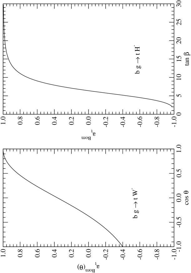
FIG. 3.: Born values of the final top quark polarization asymmetry for the two processes $bg\to tW^{-}$ or $tH^{-}$. Notice that in the first case the asymmetry is independent on $\tan\beta$, but is scattering angle dependent. In the second process, these features are reversed.

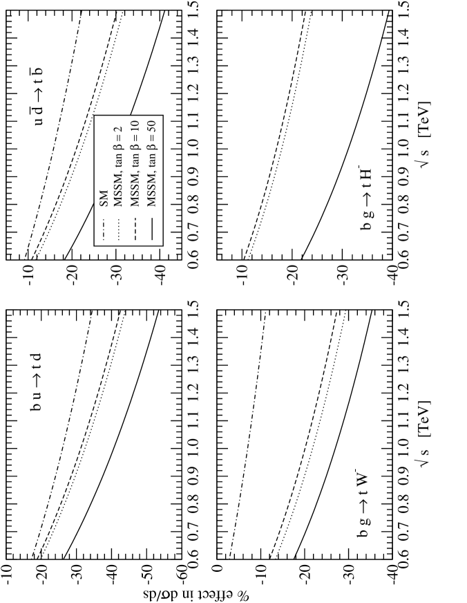
FIG. 4.: Percent correction to the (unpolarized) cross section $d\sigma/ds$ due to the full set of Sudakov logarithmic corrections. We show the curves for the Standard Model and for the MSSM at three reference values of $\tan\beta$.

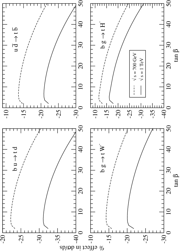
FIG. 5.: Percent correction to the (unpolarized) cross section $d\sigma/ds$ due to the full set of Sudakov logarithmic corrections. We show the curves in the MSSM as functions of $\tan\beta$ at two reference energy values $\sqrt{s}=0.7,1$ TeV.

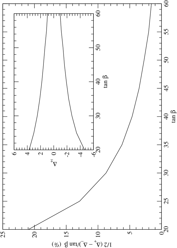
FIG. 6.: Results from the $\chi^{2}$ analysis of the $\tan\beta$ dependence of the cross sections for the processes $bu\to td$, $u\bar{d}\to t\bar{b}$ and $bg\to tW^{-}$. A 10% precision is assumed on all the three processes. For each hypothetical true value of $\tan\beta$, the figures show the $\Delta\chi^{2}=1$ boundaries $\tan\beta+\Delta_{\pm}$ (shown in the inset plot) and the corresponding relative error defined as $\frac{1}{2}(\Delta_{+}-\Delta-)/\tan\beta$. The Figure is cut at the upper limit of 25% since for larger values of the accuracy, the present derivation of the confidence bounds deserves a more detailed treatment. Actually the accuracy is minimum around $\tan\beta\simeq 6$ and is again better than $25\%$ when $\tan\beta<3$. To avoid confusion we have shown the results of the analysis for $\tan\beta>20$.

FIG. 7.: Results from the $\chi^{2}$ analysis of the $\tan\beta$ dependence of the cross sections for the process $bg\to tH^{-}$. We show the confidence limits $\tan\beta^{\pm}$ (defined in Sec. IIIA) on $\tan\beta$ and the corresponding relative bounds $(\tan\beta^{\pm}-\tan\beta)/\tan\beta$ for different choices of the theoretical representation of the cross section as discussed in the text. In more details, the left figures plots the two curves corresponding

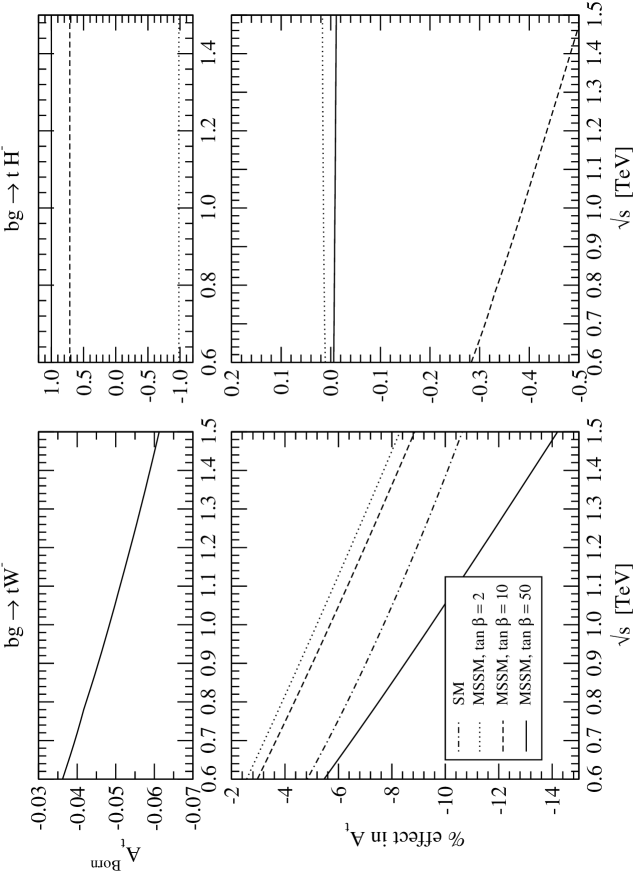
FIG. 8.: Energy dependence of the final top polarization asymmetry. In the top line, we show for the two processes $bg\to tW^{-}$, $bg\to tH^{-}$ the Born values of the asymmetry. In the bottom line, we show the percentual correction due to the full set of Sudakov logarithmic corrections. We show the curves for the Standard Model and for the MSSM at three reference values of $\tan\beta$.

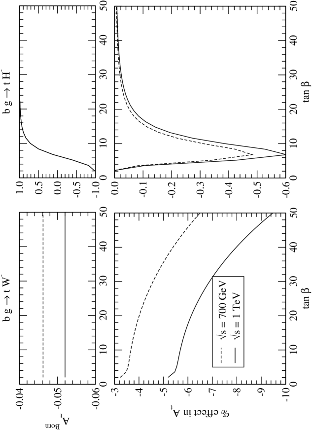
FIG. 9.: $\tan\beta$ dependence of the final top polarization asymmetry. In the top line, we show for the two processes $bg\to tW^{-}$, $bg\to tH^{-}$ the Born values of the asymmetry. In the bottom line, we show the percentual correction due to the full set of Sudakov logarithmic corrections. We show curves for the MSSM at two reference energy values $\sqrt{s}=0.7,1$ TeV.

REFERENCES

- [1] ”Top quark Physics”, M. Beneke et al, CERN-TH-2000-004, Proc. of the workshop on Standard Model physics (and more) at the LHC; editors G. Altarelli and M. L. Mangano, Geneva 2000, pag. 419.
- [2] see complete references in [1].
- [3] C.S. Li, R.J. Oakes and J.M. Yang, Phys. Rev. D55, 5780 (1997); C.S. Li, R.J. Oakes, J.M. Yang and H. Y. Zhou, Phys. Rev.D57, 2009 (1998).
- [4] A. Belyaev, D. Garcia, J. Guasch and J. Sola, JHEP 0206,059(2002); J. Guasch, P. Häfliger, M. Spira, Phys. RevD68, 115001 (2003).
- [5] E. L. Berger, Tao Han, J. Jiang and T. Plehn, hep-ph/0312286.
- [6] D.P. Roy, Mod. Phys. Lett. A19, 1813 (2004).
- [7] M. Beccaria, F. M. Renard, C. Verzegnassi, Phys. Rev. D 69, 113004 (2004), and references therein.
- [8] M. Beccaria, F.M. Renard, C. Verzegnassi, Nucl. Phys. B 663/1-2, 394 (2003).
- [9] M. Carena, D. Garcia, U. Nierste, C. E. M. Wagner, Nucl. Phys. B577, 88 (2000).
- [10] M. Beccaria, S.Bentvelsen, M.Cobal, F.M. Renard and C. Verzegnassi, to appear.
- [11] The Higgs Working Group: Summary Report 2003, By Higgs Working Group Collaboration (K.A. Assamagan et al.). June 2004. 3rd Les Houches Workshop: Physics at TeV Colliders, Les Houches, France, 26 May - 6 June 2003. hep-ph/0406152
- [12] see e.g. R.K. Ellis, W.J. Stirling and B.R. Webber, ”QCD and Colliders Physics”, Cambridge University Press, eds. T.Ericson and P.V. Landshoff (1996).
- [13] General information and updated numerical routines for parton distribution functions can be found on the www site http://durpdg.dur.ac.uk/hepdata/. The set we used is described in A.D. Martin, R.G. Roberts, W.J. Stirling, R.S. Thorne, “MRST partons and uncertainties”, contribution to XI International Workshop on Deep Inelastic Scattering, St. Petersburg, 23-27 April 2003, hep-ph/0307262.
- [14] A. Datta, A. Djouadi, and J-L. Kneur, Phys. Lett. B509, 299 (2001); J. Gunion et al., ibid. 565, 42 (2003).