OSU-HEP-04-11

October 2004

Perturbative Unification and Higgs Boson Mass Bounds
K.S. Babu^(a), Ilia Gogoladze^(b) and Christopher Kolda<sup>(b)

(a)</sup>Oklahoma Center for High Energy Physics, Department of Physics,
Oklahoma State University, Stillwater, OK  74078, USA
  
^(b)Department of Physics, University of Notre Dame
Notre Dame, IN  46556, USA

Supersymmetric extensions of the Standard Model generally give a theoretical upper limit on the lightest Higgs boson mass which may be uncomfortably close to the current experimental lower bound of $m_{h}>114$ GeV. Here we show ways in which this upper limit on $m_{h}$ can be relaxed substantially in the perturbative regime, while maintaining the successful unification of gauge couplings as observed in the minimal scenario. A class of models is presented, which includes new vector-like matter with the quantum numbers of the ${\bf 5}$, ${\bf\overline{5}}$ and singlet representations of $SU(5)$ and having Yukawa couplings ($\kappa$) to the usual Higgs doublet $H_{u}$. This new matter transforms non-trivially under a “lateral” $SU(N)$ gauge symmetry, which enables the new Yukawa couplings $\kappa$ to be sizable, even larger than the top-quark Yukawa coupling, and still be perturbative at all momenta up to the unification scale of $10^{16}\,$GeV. We find that, consistent with low energy constraints, $m_{h}$ can be raised to values as large as 200 – $300\,$GeV.

With the discovery nearly a decade ago of the top quark, the penultimate piece of the Standard Model (SM), our full attention has finally turned to the missing link – the Higgs boson. While its discovery would complete the SM, it would also bring to the forefront the study of electroweak symmetry breaking and all that comes with it (supersymmetry, extra dimensions, etc). But discovery of the Higgs boson is no simple feat. In particular, the channels in which it can be observed, and thus the methods used to find it, are highly sensitive to its mass, which remains unknown. Though there do exist constraints on $m_{h}$ from loop processes in the SM, the dependence on $m_{h}$ is logarithmic and thus small uncertainties in electroweak observables lead to exponentially larger uncertainties in the Higgs mass itself.

Within the SM, the mass of the Higgs boson is not predicted. While present analyses of the precision radiative constraints within the SM indicate a Higgs mass somewhere around 100 GeV, the model itself puts only weak constraints on $m_{h}$ from unitarity: $m_{h}\lower 3.01385pt\hbox{$\;\stackrel{{\scriptstyle\textstyle<}}{{\sim}}\;$}700\,{\rm GeV}$ [1]. Even after we embed the model in a more complete ultraviolet picture, the added constraints of vacuum stability and triviality only serve to loosely bound the Higgs mass range [2, 3].

The minimal supersymmetric extension of the SM (the MSSM) is another story. It is well known that the mass of the lightest Higgs boson of the MSSM is bounded at tree level by the $Z^{0}$ mass. Radiative corrections can push the mass higher, but only to about 125 to $130\,{\rm GeV}$ for $M_{\rm SUSY}\lower 3.01385pt\hbox{$\;\stackrel{{\scriptstyle\textstyle<}}{{\sim}}\;$}1\,{\rm TeV}$. (Here $M_{\rm SUSY}$ represents the average mass of the top squarks.) As experiments have pushed the lower mass bound on the Higgs higher and higher, the parameter space for SUSY has been pushed further and further into corners in which top squarks are heavy and left-right mixing is large. In essence, even small increases in the experimental bound on $m_{h}$ lead to large increases in the tuning required to make the MSSM consistent with experiment [4].

Many groups have examined ways to extend the MSSM in order to push up the lightest Higgs mass and partially evade the tuning issues [5]. Generally speaking, the farther one is willing to move away from the basic picture of the MSSM, the higher one is able to push the Higgs mass. Models which add only a few extra matter representations, or additional Higgs multiplets, succeed only in raising the Higgs mass bound by a few to few tens of GeV. However there are models which look nothing like the MSSM in the ultraviolet, involving for example new strong dynamics in which the MSSM degrees of freedom are no longer fundamental. In such models the upper bound on $m_{h}$ can be extended by hundreds of GeV.

In this paper, we would like to keep the best of both worlds – minimality but with a large effect. We will present a model (actually a class of models) in which very large corrections to the Higgs mass can occur, while remaining as close as possible to the spectrum and interactions of the MSSM. In particular, we wish to preserve a property of the MSSM which we consider too valuable to abandon, namely gauge coupling unification which occurs at scales sufficiently large to prevent fast proton decay.

This last property is really two independent requirements, both of which are met in the MSSM: first, that the gauge couplings unify numerically and perturbatively, and second that they unify at a sufficiently large scale that the resulting dimension-6 nucleon decay rates are consistent with proton lifetime bounds. If we are to consider the unification in the MSSM as more than a coincidence then there are only a few possible extensions which we may consider: the addition of gauge singlets fields, as in the NMSSM [6, 7]; the addition of new matter fields whose quantum numbers fit into complete SU(5) representations [8]; or the addition of new interactions commuting with the usual gauge groups [9].

Of these, the first two have been considered in detail by others and the last only in passing (since it usually does not help). We consider all three in tandem and show that we can generate Higgs masses far above those predicted in the MSSM. Because the quantum numbers of the new matter will allow it to couple to the $H_{u}$ field, the new Yukawa couplings will generate large corrections to the light Higgs mass in much the same way that the top quark/squark loops do in the MSSM. But as we will see, the Yukawa coupling can be appreciably larger than the top Yukawa of the MSSM, consistent with perturbative unification, and so the corrections can be extremely large.

Higgs Mass in the MSSM

Before discussing our model, let us briefly review the calculation of $m_{h}$ in the MSSM and its concomitant problems. At tree level, the lightest scalar Higgs mass is bounded from above by $m_{h}\leq m_{Z}\cos 2\beta$. The bound is saturated in the decoupling limit where the pseudoscalar Higgs mass is taken to infinity: $m_{A}\to\infty$. In determining the upper bound in $m_{h}$, we will take this limit for the remainder of the paper.

There are several large corrections to this bound, but they are essentially dominated by terms in the effective potential of the form $(H_{u}^{\dagger}H_{u})^{2}$. These corrections have been calculated by a large number of authors and reviewed already in several other papers [10, 11]. Nonetheless we remind the reader of the leading 1- and 2-loop contributions:

$$m_{h}^{2} = m_{Z}^{2}\cos^{2}2\beta\left(1-\frac{3}{8\pi^{2}}\frac{m_{t}^{2}}{v^{2}}\ t\right)$$

$$+ \frac{3}{4\pi^{2}}\frac{m_{t}^{4}}{v^{2}}\left[t+\frac{1}{2}X_{t}+\frac{1}{16\pi^{2}}\left(\frac{3}{2}\frac{m_{t}^{2}}{v^{2}}-32\pi\alpha_{s}\right)\left(X_{t}t+t^{2}\right)\right].$$

Here $v=174\,{\rm GeV}$ is the usual SM Higgs vev and $t=\log(M_{\rm SUSY}^{2}/m_{t}^{2})$. The first term in square brackets is the famously large ($\sim m_{t}^{4}$) correction to the light Higgs mass, while the first term in parenthesis is a smaller D-term contribution. The terms proportional to $X_{t}$ are corrections due to left-right top squark mixing. Here $X_{t}$ is defined as

$$X_{t}=\frac{2\tilde{A}_{t}^{2}}{M_{\rm SUSY}^{2}}\left(1-\frac{\tilde{A}_{t}^{2}}{12M_{\rm SUSY}^{2}}\right)$$ (2)

where $\tilde{A}_{t}=A_{t}-\mu\cot\beta$ is the top squark mixing parameter. The remaining terms in Eq. (Higgs Mass in the MSSM) are the leading 2-loop effects, which we will keep throughout this analysis.

The size of the corrections is logarithmically dependent on the “cut-off” which is here the mass scale of the top squarks: $M_{\rm SUSY}\simeq m^{2}_{\tilde{t}_{1},\tilde{t}_{2}}$. For simplicity (and following standard conventions) we will take all squarks to be degenerate, apart from mass splittings induced by mixing. To find an upper bound on $m_{h}$ is it customary to take $M_{\rm SUSY}$ as large as possible consistent with our prejudices about fine tuning. Usually this means taking $M_{\rm SUSY}=1\,{\rm TeV}$. Using that value, one finds for the unmixed case ($X_{t}=0$) that $m_{h}<110\,{\rm GeV}$. The light Higgs mass is maximized for the case $X_{t}=6$ (or $A_{t}=\sqrt{6}M_{\rm SUSY}$) where one find $m_{h}<125\,{\rm GeV}$. These two extrema are usually referred to as the minimal and maximal mixing scenarios.

Current experimental constraints on $m_{h}$ already rule out a substantial portion of the mass range of the light Higgs. For large $m_{A}$, the SM Higgs bound translates directly over to the MSSM and one has $m_{h}>114\,{\rm GeV}$ at 90% CL [12].

One can turn this around and ask how large $M_{\rm SUSY}$ must be in order to conform to experiment. For example, if $A_{t}=0$ one finds that $M_{\rm SUSY}\geq 1.5\,{\rm TeV}$. Such a large value for $M_{\rm SUSY}$ will induce rather large corrections (of $O(\,{\rm TeV})$) for the mass parameters in the Higgs potential. In order to generate a vev of $174\,{\rm GeV}$, one must assume a delicate cancellation, either between the $\mu$-term and the Higgs mass parameters, or between the bare mass parameters and their one-loop corrections [4]. In either guise, this tuning (usually called the “little hierarchy problem”) has led many theorists to consider ways to extend the MSSM in order to push up $m_{h}$ [5].

We will be doing something similar but not exactly the same. Our goal is not to solve this little hierarchy problem, but rather to ask how far we can push the Higgs mass consistent with phenomenological bounds and gauge coupling unification. Some of the parameter space we are considering will require fine-tuning as in the little hierarchy problem, some will not, as we will discuss later.

The Model: Extra Matter

It has long been understood that one can extend the matter sector of the MSSM and still preserve the beautiful result of gauge coupling unification if the new matter falls into complete multiplets of SU(5). That is, the quantum numbers of the new matter must exactly fill up representations of SU(5); there is no need for SU(5) to be respected by the interactions, just by the matter content. Such complete, but light, GUT multiplets are not unexpected. Within string theory one often finds light multiplets in the spectrum. And even within the framework of GUTs themselves one can find extra complete multiplets lying at the weak scale [13]. In particular, if a symmetry prevents a multiplet from receiving a GUT-scale mass, that multiplet will then usually get its mass from SUSY-breaking effects, which naturally places it at the weak scale.

However there are stringent constraints on new light matter from a number of sides. Most important are the constraints from the $S$ and $T$ parameters which limit the number of additional chiral generations. Consistent with these constraints, one must add new matter which is predominantly vector-like and only has a chiral mass which is subdominant.

Since the smallest representations of SU(5) are chiral, we must therefore introduce them in pairs (e.g., ${\bf 5}+{\bf\overline{5}}$ or ${\bf 10}+{\bf\overline{10}}$) in order to allow explicit mass terms. But we must also allow for the possibility that these fields couple to the Higgs fields of the MSSM. For example, with a ${\bf 10}+{\bf\overline{10}}$ a mass term of the form ${\bf 10}\cdot{\bf 10}\cdot H_{u}$ is allowed. If we allow SM singlets, then Dirac mass terms of the form ${\bf\overline{5}}\cdot S\cdot H_{u}$ and ${\bf 5}\cdot S\cdot H_{d}$ are also permitted.

How large can the new Yukawa couplings be? There are two severe constraints. The first comes from the $T$ parameter. In the limit $M_{V}\gg M_{D}$, the contribution from a single chiral fermion is approximately [14]:

$$T=\frac{N(\kappa v)^{2}}{10\pi\sin^{2}\theta_{W}m^{2}_{W}}\left[\left(\frac{\kappa v}{M_{V}}\right)^{2}+O\left(\frac{\kappa v}{M_{V}}\right)^{4}\right]$$ (3)

where $\kappa$ is the new Yukawa coupling, $v$ is vev of corresponding Higgs field, and $N$ counts the additional degrees of freedom possessed by the new field. Precision electroweak data constrains $T=-0.17\pm 0.12$ for $m_{h}=117\,{\rm GeV}$ or $-0.08\pm 0.12$ for $m_{h}=300\,{\rm GeV}$ [12]. As a figure of merit, we will take $T<0.1$ as a realistic bound and apply it in our analysis. Then it is easy to see from Eq. (3) that when $M_{V}$ is around 1 TeV the Yukawa coupling $\kappa$ can be $O(1)$!

The second constraint comes from perturbativity and unification. If we are to maintain natural gauge coupling unification, then we must also maintain perturbativity of the gauge and Yukawa couplings at all scales below $M_{\rm GUT}$. A new $O(1)$ coupling presents a problem both in its own evolution towards the GUT scale, but also in its effect on the running of the top quark Yukawa, which is already known to be near its quasi-fixed point. Since the self-coupling of any new Yukawa would drive that same Yukawa up in the ultraviolet, and may also drive up $y_{t}$, the new Yukawa coupling cannot be too large. For example, the ${\bf 10}\cdot{\bf 10}\cdot H_{u}$ coupling cannot be larger than $1.1$. Even worse, the ${\bf\overline{5}}\cdot S\cdot H_{u}$ coupling cannot be larger than $0.75$.

Perturbativity and unification also bound the amount of new matter than can be added to the MSSM, since each new representation increases the gauge $\beta$-functions. One finds that one can safely add to the low-energy (TeV-scale) spectrum only the following: (i) up to 4 pairs of $({\bf 5}+{\bf\overline{5}})$’s, or (ii) one pair of $({\bf 10}+{\bf\overline{10}})$, or (iii) one pair of each, $({\bf 5}+{\bf\overline{5}}+{\bf 10}+{\bf\overline{10}})$. The last option of course also fits nicely into an SO(10) model. In addition, any number of gauge singlets can be added without upsetting unification or perturbativity.

Cases (ii) and (iii) have been studied extensively before. For example, Moroi and Okada [8] concluded that the mass of the lightest CP even Higgs mass could be pushed up as high as 160 GeV consistent with all perturbativity constraints.

By itself, case (i) does not allow for any new Yukawa coupling unless the new states in the ${\bf\overline{5}}$ are mixed into the usual $d$-quarks and leptons. Such a possibility is even more strongly constrained (by flavor violation and unitarity of the CKM matrix, among others) and so we will forbid all such mixing. In the next section an explicit argument for doing so will appear.

But we can generate new Yukawa couplings for case (i) if we introduce gauge singlet fields $S$ and $\overline{S}$ which couple to the usual Higgs bosons as ${\bf\overline{5}}\cdot\overline{S}\cdot H_{u}$ and ${\bf 5}\cdot S\cdot H_{d}$. More explicitly, we decompose the ${\bf 5}$ as $(d^{\prime},\overline{L}^{\prime})$ and ${\bf\overline{5}}$ as $(\overline{d}^{\prime},L^{\prime})$, where $d^{\prime}$ and $L^{\prime}$ have the same quantum numbers as the $d_{R}$-quarks and $L_{L}$ leptons of the SM. Then we generate a superpotential with only two new Yukawa interactions. For one pair of ${\bf 5}+{\bf\overline{5}}$ and one pair of singlets $S+\overline{S}$, the superpotential is:

$$W=\kappa L^{\prime}\overline{S}H_{u}+\kappa^{\prime}\overline{L}^{\prime}SH_{d}+M_{V}(\overline{S}S+\overline{L}^{\prime}L^{\prime}+\overline{d}^{\prime}d^{\prime})$$ (4)

where we have taken a common vector-like mass for simplicity. Thus the lepton-like pieces of the ${\bf 5}$ and ${\bf\overline{5}}$ get Dirac and vector-like masses, while leaving the $d$-quark-like pieces with only vector-like masses.

Because the new matter couples to the SM Higgs fields, they will generate radiative corrections in much the same way as the top quark and squarks. And like the top/bottom sector, the coupling to $H_{u}$ will play a much more dominant role in those corrections than the coupling to $H_{d}$, assuming $\tan\beta>1$. This is important because both the $\kappa$ and $\kappa^{\prime}$ couplings will tend to run to large values in the ultraviolet. For example, if we have $N$ pairs of ${\bf 5}+{\bf\overline{5}}$ and if all couple with the same strength $\kappa$ then:

$$\frac{d}{d\log Q}\kappa=\frac{\kappa}{16\pi}\left[(3+N)\kappa^{2}+3y_{t}^{2}-\left(\frac{3}{5}g_{1}^{2}+3g_{2}^{2}\right)\right].$$ (5)

Of perhaps even greater importance is the RGE for $y_{t}$, which has a new contribution proportional to $\kappa^{2}$:

$$\frac{d}{d\log Q}y_{t}=\left[\frac{d}{d\log Q}y_{t}\right]_{\rm MSSM}\!+\frac{N}{16\pi^{2}}y_{t}\kappa^{2}.$$ (6)

Because $\kappa$ and $y_{t}$ are coupled through their RGEs, $\kappa$ is more tightly constrained than $\kappa^{\prime}$. However the mass of the lightest Higgs, $h^{0}$, is much more sensitive to $\kappa$ than it is to $\kappa^{\prime}$. Furthermore, very large values of $\kappa^{\prime}$ will actually drive the Higgs mass down. Therefore we will take $\kappa^{\prime}=0$ for the remainder of this work.

Running the RGEs for $\kappa$ and $y_{t}$ from the weak scale to the GUT scale (which we take as $2\times 10^{16}\,{\rm GeV}$), we find an upper bound on $\kappa$ of $0.75$ for $N=1$ and $0.65$ for $N=3$ (assuming $\tan\beta\gg 1$). Calculating the correction to the Higgs mass (formulas to follow in next section) yields a new upper bound on $m_{h}$ which is at most $20\,{\rm GeV}$ above the MSSM limit, not much of an improvement.

Of course the correction to $m_{h}^{2}$ scales as $\kappa^{4}$, so if we were able to significantly increase the low-energy value of $\kappa$ we could generate much larger Higgs masses, as we will now see.

The Lateral Gauge Symmetry

Models with extra pairs of $({\bf 5}+{\bf\overline{5}})$’s present one extra degree of freedom in model building. Specifically, if one has $N$ pairs of ${\bf 5}+{\bf\overline{5}}$ then one can impose on them a new $SU(N)$ symmetry under which the SM particles are uncharged. As a global symmetry, this $SU(N)$ only serves to constrain the forms of the couplings; for example, it would prevent mixing between the vector-like quarks and the ordinary quarks unless the symmetry is broken.

As a gauge symmetry, there are new opportunities for generating large corrections to $m_{h}$. Because it is reminiscent of “horizontal” symmetries among the quark generations, we will call this a “lateral” symmetry and denote it $SU(N)_{\ell at}$. Because of perturbativity there are only three possible lateral symmetry groups: $SU(2)$, $SU(3)$ and $SU(4)$. ($Sp(4)$ is another possible group, but we will not consider it.) We will keep most of our discussion general with respect to $N$, but our numerical work will be done for $N=3$ just to be specific.

The non-MSSM matter content is then as follows, with the charges under $SU(3)_{c}\times SU(2)_{W}\times SU(N)_{\ell at}\times U(1)_{Y}$ shown:

$$d^{\prime}\,({\bf 3},{\bf 1},{\bf N})_{1/3}, \overline{d}^{\prime}\,({\bf\overline{3}},{\bf 1},{\bf\overline{N}})_{-1/3},$$

$$L^{\prime}\,({\bf 1},{\bf 2},{\bf N})_{1/2}, \overline{L}^{\prime}\,({\bf 1},{\bf 2},{\bf\overline{N}})_{-1/2},$$ (7)

$$S\,({\bf 1},{\bf 1},{\bf N})_{0}, \overline{S}\,({\bf 1},{\bf 1},{\bf\overline{N}})_{0}.$$

The superpotential is again given by Eq. (4). Again we will take $\kappa^{\prime}\to 0$, which has very little effect on our limits.

The major advantage of gauging the lateral symmetry comes in the RGEs for $\kappa$. Let us reiterate that in order to maximize the Higgs mass correction, we want $\kappa$ to be as large as possible at the weak scale. However a large $\kappa$ enters the RGE for $y_{t}$, driving it to an ultraviolet instability long before the GUT scale. Furthermore the $\beta$-function for $\kappa$ itself is positive, which means that a large $\kappa$ in the infrared only becomes larger, and more troublesome, in the ultraviolet.

Gauging the lateral symmetry changes all this because now one finds:

$$\frac{d}{d\log Q}\kappa=\frac{\kappa}{16\pi}\left[(3+N)\kappa^{2}+3y_{t}^{2}-\left(\frac{3}{5}g_{1}^{2}+3g_{2}^{2}+4C_{2}^{\ell at}g_{{\ell at}}^{2}\right)\right]$$ (8)

where $C_{2}^{\ell at}$ is the quadratic Casimir for the fundamental representation of $SU(N)_{\ell at}$: $C_{2}^{\ell at}=(N^{2}-1)/2N$. The RGE for the new coupling $g_{\ell at}$ or $\alpha_{\ell at}$ is simply:

$$\frac{d}{d\log Q}\alpha_{\ell at}=\frac{1}{2\pi}\beta_{\ell at}\,\alpha^{2}_{\ell at}$$ (9)

where $\beta_{\ell at}$ is the numerical $\beta$-function coefficient, to be determined.

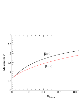
How does $\alpha_{\ell at}$ help? In Eq. (8) it is the gauge pieces that drive down $\kappa$ in the ultraviolet, preventing $\kappa$ from hitting its Landau pole. More importantly they suppress the contributions of $\kappa$ to the running of $y_{t}$. Thus much larger values of $\kappa$ are possible for non-zero $\alpha_{\ell at}$. In Fig. 1 we graph the upper bound on $\kappa$ as a function of $\alpha_{\ell at}$ for $N=3$ and two cases of $\beta$: $\beta_{\ell at}=0$ and $-3$. Just as the top quark corrections to $m_{h}^{2}$ scale as $y_{t}^{4}$, so too these new corrections scale as $\kappa^{4}$. So it would appear that larger $\alpha_{\ell at}$ immediately leads to larger $m_{h}$, and to a good approximation this is correct, though not complete.

Figure 1: Plot of maximum allowed $\kappa$ as a function of $\alpha_{\ell at}$ for the $N=3$ case with $\beta_{\ell at}=0$ and $-3$.

We are finally in a position to give the expression for the radiative correction to $m_{h}^{2}$ coming from the new matter:

$$m_{h}^{2} = \left[m_{h}^{2}\right]_{MSSM}-m_{Z}^{2}\cos^{2}2\beta\left(\frac{N}{8\pi^{2}}\kappa^{2}\ t_{1}\right)$$

$$+ N\kappa^{4}\frac{v^{2}\sin^{4}\beta}{4\pi^{2}}\left[t_{1}+\frac{1}{2}X_{\kappa}+\frac{1}{16\pi^{2}}\left(\frac{N}{2}\kappa^{2}-6C_{2}^{\ell at}g^{2}_{\ell at}\right)\left(X_{\kappa}t_{1}+t_{1}^{2}\right)\right].$$

where

$$t_{1}=\log\left(\frac{M^{2}_{SUSY}+M_{V}^{2}}{M_{V}^{2}}\right)$$ (11)

and we have assumed $M_{V}\gg M_{D}$. Here $X_{\kappa}$ is analogous to $X_{t}$ in the stop sector:

$$X_{\kappa}=\frac{2\tilde{A}_{\kappa}^{2}}{M_{\rm SUSY}^{2}+M_{V}^{2}}\left(1-\frac{1}{12}\frac{\tilde{A}_{\kappa}^{2}}{M_{\rm SUSY}^{2}+M_{V}^{2}}\right)$$ (12)

where $\tilde{A}_{\kappa}=A_{\kappa}-\mu\cot\beta$ is the $L^{\prime}$–$\overline{S}$ soft mixing parameter.

We learn several things from the form of Eq. (The Lateral Gauge Symmetry). First, it is clear that the corrections grow as $\kappa^{4}$, so large $\kappa$ will generate large Higgs masses. Second, we notice that the 2-loop piece contains terms suppressed by $\alpha_{\ell at}$, so for sufficiently large $\alpha_{\ell at}$, the 2-loop suppression of $m_{h}^{2}$ offsets the enhancements generated by the $\alpha_{\ell at}$-dependence in the RGEs.

We have outlined here a broad class of models which can significantly increase the SUSY light Higgs mass. Each model is described by only a few free parameters: $N$, the number of $({\bf 5}+{\bf\overline{5}})$ multiplets; $M_{V}$, the explicit, SUSY-preserving mass of those multiplets; $M_{\rm SUSY}$, the soft-breaking mass scale; $\kappa$, the Yukawa coupling of the new matter to $H_{u}$; $\alpha_{\ell at}$, the strength of the new $SU(N)$ gauge interaction; $\beta_{\ell at}$, the $\beta$-function for $\alpha_{\ell at}$; and of course $\tan\beta$, the ever-present ratio of the Higgs vevs. As in the MSSM, there is also a dependence on the left-right mixing parameters, $\tilde{A}_{t}$ and $\tilde{A}_{\kappa}$, which explicitly appear in the Higgs mass correction.

In what follows we will study one particular subclass of models in order to show the power of this approach for lifting the Higgs mass predictions.

The $SU(3)_{\ell at}$ Case

Now we turn our attention to one choice of $N$, namely $N=3$. Our choice is not dictated by any exceptionally deep reason. One could argue that the $N=3$ case fits nicely into an $E_{6}$ unified picture (where there is an extra pair of ${\bf 5}+{\bf\overline{5}}$ in each 27) and is therefore preferred. But the $SU(3)_{\ell at}$ case will also highlight all the key points we wish to make.

The matter content (Eq. (7)) and superpotential (Eq. (4)) of the $SU(3)_{\ell at}$ model both follow from the discussion in the previous sections. As before we will make two simplifying assumptions: that all new matter receives a universal vector-like mass $M_{V}$ and that all SUSY scalars receive a universal scalar mass $M_{\rm SUSY}$. Deviations from these assumptions will have only a negligible effect on the derived bound on $m_{h}$.

What is not immediately obvious is what we should take for $\beta_{\ell at}$. The minimal model yields $\beta_{\ell at}=-3$. In such a model all the matter charged under $SU(3)_{\ell at}$ would be integrated out at the scale $M_{V}$. In the infrared the only remaining degrees of freedom would be gauge and would thus form “lateral glueballs” which would not have direct interactions with SM matter.

On the other hand, it would be natural for the model to contains Higgs fields to break the lateral symmetry. A model with three Higgs fields, each in the fundamental of $SU(3)_{\ell at}$, along with their conjugates would break the lateral symmetry completely. The resulting model would have $\beta_{\ell at}=0$. Of course, any additional matter would turn $\beta_{\ell at}>0$.

This brings us to an interesting question: could an Abelian symmetry work for us? The answer is no. As we will see shortly, at the weak scale we require the lateral interaction to be fairly strong in order to stabilize the RGE flow of $\kappa$ and $y_{t}$. An Abelian symmetry would have positive $\beta$-function and so the strongly coupled lateral group would become non-perturbative in the ultraviolet.

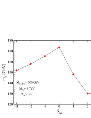
On the other hand, a negative $\beta$-function allows $\alpha_{\ell at}$ to be large in the infrared, but suppresses it in the ultraviolet so that its dampening effect on the running of $\kappa$ is vitiated. Logically it seems that $\beta_{\ell at}=0$ maximizes the effect that $\alpha_{\ell at}$ has on the Higgs mass calculation, a deduction borne out by the numerical calculation shown in Fig. 2 where explicit dependence on the $\beta$-function is shown. In this figure we have plotted the upper bound on $m_{h}$ as a function of $\beta_{\ell at}$ for $M_{\rm SUSY}=500\,{\rm GeV}$ and $M_{V}=1\,{\rm TeV}$. We require in this one plot that $\alpha_{\ell at}(m_{Z})<0.3$ and that $\alpha_{\ell at}$ remains perturbative all the way to the GUT scale. The plot clearly shows $\beta=0$ as a maximum. However all $\beta\leq 0$ are interesting and give sizable enhancements to $m_{h}$. Positive $\beta$-functions help very little, since they drive $\alpha_{\ell at}$ non-perturbative in the ultraviolet and thus necessitate lower values of $\alpha_{\ell at}$ at the weak scale.

Figure 2: Plot of maximum allowed Higgs mass, $m_{h}$, as a function of $\beta_{\ell at}$ for $SU(3)_{\ell at}$ with $M_{\rm SUSY}=500\,{\rm GeV}$, $M_{V}=1\,{\rm TeV}$ and $\alpha_{\ell at}(m_{Z})<0.3$.

Our central result is then the maximization of $m_{h}$ as a function of $\alpha_{\ell at}$. We leave $\alpha_{\ell at}$ as a free variable since there is a strong dependence on its value. We also leave $M_{\rm SUSY}$ free since we have no a priori reason to choose $200\,{\rm GeV}$ rather than $1\,{\rm TeV}$. And we choose $\beta_{\ell at}=0$ and $-3$.

How large can $\alpha_{\ell at}$ be before our perturbative calculation of the Higgs mass begins to fail? Because we assume $\beta_{\ell at}\leq 0$, there is no problem with perturbativity in the ultraviolet. Furthermore, in the calculation of the new contributions to $m_{h}^{2}$, the proper expansion parameter is not $\alpha_{\ell at}$, but rather $\alpha_{\ell at}/4\pi$. This is analogous to the QCD contributions to leptonic magnetic moments. Thus our calculation of $m_{h}$ should work reasonably well even for values of $\alpha_{\ell at}$ much larger than $\alpha_{\rm QCD}(m_{Z})$.

In any case, our numerical procedure is simple: For a given value of $\alpha_{\ell at}$ and $M_{\rm SUSY}$, we vary $M_{V}$ and $\kappa$ over their allowed ranges in order to maximize $m_{h}$. The minimum for $M_{V}$ is set by requiring $T<0.1$; this will of course depend on $\kappa$. The upper bound for $M_{V}$ we choose to be $2\,{\rm TeV}$ arbitrarily. While there is no lower bound on $\kappa$, the upper bound is set by requiring the values of $y_{t}(Q)$ and $\kappa(Q)$ remain perturbative at all scales $Q\leq M_{\rm GUT}$.

We have thus far avoided discussing the left-right mixing parameters. It turns out that these play a crucial role. It is well known that in the MSSM, the Higgs mass is maximized for $X_{t}=6$, or equivalently $\tilde{A}_{t}=\sqrt{6}M_{\rm SUSY}$. For fields with both chiral and vector-like masses, the form of $X$ is altered to that of Eq. (12). The one-loop corrections are maximized for $X_{\kappa}=6$, however it may not be possible to reach such large values. In fact, there are really two distinct cases to be considered, both of which are physically acceptable, though one may (or may not) be considered more natural than the other.

The first case is to require that $A_{\kappa}$ scales with $M_{\rm SUSY}$. For example, in the MSSM the requirement that there be no charge- or color-breaking minima in the scalar potential lower than the SM minimum gives us the usual [15]:

$$A_{t}^{2}\leq 3\left(m^{2}_{\tilde{t}_{L}}+m^{2}_{\tilde{t}_{R}}+m^{2}_{H_{u}}\right).$$ (13)

Since $m^{2}_{H_{u}}<0$ usually, then we can rewrite this as $|A_{t}|<\sqrt{6}M_{\rm SUSY}$, assuming $m_{\tilde{t}_{L}}=m_{\tilde{t}_{R}}=M_{\rm SUSY}$. Thus we might also expect that

$$|A_{\kappa}|<\sqrt{6}M_{\rm SUSY}.$$ (14)

However, because of the presence of the $M_{V}$ mass term, Eq. (14) generalizes to:

$$A_{\kappa}^{2}<6\left(M_{V}^{2}+M_{\rm SUSY}^{2}\right)$$ (15)

which allows for much larger values of $A_{\kappa}$ and thus $X_{\kappa}$. There are theoretical arguments both for and against loosening the constraint of Eq. (14) to that of Eq. (15). Since $M_{V}$ is a priori independent of $M_{\rm SUSY}$, there is no good reason for a soft-breaking parameter like $A_{\kappa}$ to scale with $M_{V}$. And in fact, for $M_{V}\sim 2\,{\rm TeV}$, Eq. (15) would allow $A_{\kappa}$ as large as $5\,{\rm TeV}$. Even if such a large $A$-term were allowed phenomenologically, it would generate a very large fine-tuning in the soft parameters of the Higgs potential. On the other hand, it would be natural for $M_{V}$ to be associated with the SUSY-breaking scale, just as the usual $\mu$-term is presumed to be. So $A_{\kappa}$ scaling with $M_{V}$ may not be as unreasonable as it first appears. In either case, we will remain agnostic and show the limits under the constraints of Eqs. (14) and (15) both.

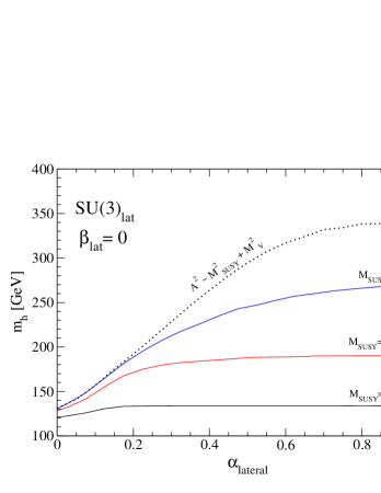
We are now prepared to calculate the Higgs mass in our lateral $SU(3)$ model. In Fig. 4 we plot the maximum Higgs mass that can be obtained as a function of $\alpha_{\ell at}$ and for given values of $M_{\rm SUSY}$. The lower three lines in the figure assume that $A^{2}_{\kappa}\sim M_{\rm SUSY}^{2}$ (that is, we impose Eq. (14)). Each line represents a maximum value of $m_{h}$ consistent with a given $M_{\rm SUSY}$. These points are maxima in the following sense. First, the stop mass correction has been maximized by assuming $X_{t}=6$ for the stops. Second, at each point along the curves, the vector-like mass, $M_{V}$, has been allowed to vary within the range

$$500\,{\rm GeV}\leq M_{V}\leq 2\,{\rm TeV}$$ (16)

in order to maximize the size of the corrections. The lower bound in Eq. (16) has been chosen to satisfy the $T$-parameter constraint, and the upper bound ensures that the vector-like matter does not decouple completely. The dependence of $m_{h}$ on $M_{V}$ is what one would expect from an examination of Eq. (The Lateral Gauge Symmetry). For $\alpha_{\ell at}$ small, it is advantageous to have as large a logarithmic enhancement as possible and so $M_{V}$ should be small. For $\alpha_{\ell at}$ large, the 2-loop corrections push down $m_{h}$ if the log is large, and so it is best to have a small log, which requires $M_{V}$ to be large. One finds $M_{V}\approx 500\,{\rm GeV}$ at $\alpha_{\ell at}=0$ and $M_{V}\approx 2\,{\rm TeV}$ when $\alpha_{\ell at}\to 1$. This effect is further enhanced by the $T$-parameter constraint: larger $\alpha_{\ell at}$ allow larger $\kappa$ which are consistent with $T$ only if $M_{V}$ is larger, and vice-versa.

Figure 3: Plot of maximum allowed Higgs mass, $m_{h}$, as a function of $\alpha_{\ell at}$ for $SU(3)_{\ell at}$ with $\beta=0$. The three lower lines assume $A^{2}\sim M_{\rm SUSY}^{2}$ and $M_{\rm SUSY}=200$, 500, and $1000\,{\rm GeV}$ respectively. The topmost dotted line represents the limit if $A^{2}\sim M_{\rm SUSY}^{2}+M_{V}^{2}$ (and is roughly indepedent of $M_{\rm SUSY}$ itself).

Figure 4: Plot of maximum allowed Higgs mass, $m_{h}$, as a function of $\alpha_{\ell at}$ for $SU(3)_{\ell at}$ with $\beta=-3$. The lines follow those in Fig. 4.

Obviously there is a strong dependence on $\alpha_{\ell at}$, which is to be expected. As $\alpha_{\ell at}$ grows, the running of $\kappa$ is suppressed and so larger weak-scale values of $\kappa$ are consistent with our perturbativity constraints. Of course, as $\alpha_{\ell at}$ grows the weak scale model itself becomes less and less perturbative. However we feel that there should be no problem trusting the calculation of the Higgs mass correction even at relatively large values of $\alpha_{\ell at}$. As a check, we have compared the size of the one-loop corrections to those at two loops and find the two-loop corrections to be uniformly small compared to the one-loop pieces, usually only 5% to 20% of the latter. Although our calculation appears to be trustworthy up to at least $\alpha_{\ell at}\simeq 1$, one need only go up to $\alpha_{\ell at}\simeq 0.3$ in order to generate large corrections to $m_{h}$.

We note a few interesting features in Fig. 4. For $\alpha_{\ell at}=0$, one reproduces the upper bounds on the Higgs mass in the MSSM: 121, 128 and $131\,{\rm GeV}$ for $M_{\rm SUSY}=200$, 500 and $1000\,{\rm GeV}$ respectively. For $\alpha_{\ell at}$ as small as $0.118$ (the value of $\alpha_{s}$ at $m_{Z}$), one already finds the Higgs mass pushed up to 125, 150, and $160\,{\rm GeV}$ for those same values of $M_{\rm SUSY}$. All of these values are well above the current mass bounds. But it is as $\alpha_{\ell at}$ gets larger that the new matter really affects the calculation. For $\alpha_{\ell at}=0.3$, the bounds on $m_{h}$ rise to 134, 181 and $213\,{\rm GeV}$.

Why is there a large dependence on $M_{\rm SUSY}$? One would naively expect that this is due to the logarithmic dependence on $M_{\rm SUSY}$ in the radiative corrections, but that is not the case. Most of the effect here is due to the left-right mixing of the new matter. But if we require $A_{\kappa}^{2}\sim M_{\rm SUSY}^{2}$ (Eq. (14)) the mixing cannot be close to maximal unless $M_{\rm SUSY}$ is large. (Recall that extra $M_{V}^{2}$ suppression in the denominator of Eq. (12).) This is the dominant source of the $M_{\rm SUSY}$ dependence.

There is one other line present in Fig. 4. The topmost, dotted line represents the limit on $m_{h}$ when $A^{2}$ is allowed to scale with $M_{\rm SUSY}^{2}+M_{V}^{2}$. Now the mixing can become maximal and $X_{\kappa}$ can approach the magic value of 6. In this case, there is almost no depedence on $M_{\rm SUSY}$ and so we show the bound as a single line. Notice that for $\alpha_{\ell at}\lower 3.01385pt\hbox{$\;\stackrel{{\scriptstyle\textstyle<}}{{\sim}}\;$}0.2$, there is no real difference between the smaller and larger values of $A_{\kappa}$. But for $\alpha_{\ell at}=0.3$ the Higgs mass bound has been pushed up from 213 to $230\,{\rm GeV}$ by the larger $A_{\kappa}$ values.

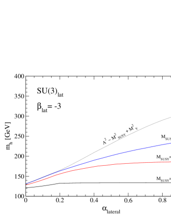
Hidden in these plots is the dependence of our result on the lateral gauge $\beta$-function. If we take $\beta=0$ we are in fact maximizing the Higgs mass. We can see this for one particular case in Fig. 4 where we plot the maximal values of $m_{h}$ as a function of $\alpha_{\ell at}$ just as in Fig. 4, but now with $\beta_{\ell at}=-3$ (the minimal model case). Notice that these bounds are lower than those for $\beta_{\ell at}=0$, particularly at large $\tan\beta$. However, the difference is not great, and we would claim that the $\beta=-3$ model is also successful at lifting the Higgs mass well above the experimental limits.

Conclusions

The famous upper bound on the Higgs mass in the MSSM may turn out to be one of the major stumbling blocks of the model and one of our best clues on how to extend it. While it is relatively simple to extend the MSSM to push the upper bound on $m_{h}$ up a few ten’s of GeV, larger changes usually require radical alterations of the model which do not allow automatic GUT-like unification and suppression of dimension-6 proton decay operators. We have shown here that it is possible to extend the MSSM in a relatively minimal way and still obtain Higgs boson masses as heavy as 200 to $300\,{\rm GeV}$. And we have done so while preserving gauge coupling unification at scales around $10^{16}\,{\rm GeV}$.

The theoretical price to be paid depends on the enhancement desired. For the largest masses, one needs either large $M_{\rm SUSY}$ or large $L^{\prime}$–$\overline{S}$ mixing through the $A_{\kappa}$ term. Either choice reintroduces the “little hierarchy” problem since the low-energy Higgs potential is sensitive to these mass scales. There is also a “$\mu$-problem” associated with setting $M_{V}$ near the weak scale, but this is presumably solved in the same way that the usual $\mu$-problem is solved. But most importantly, these models are phenomenologically consistent and do not require any radical changes in the MSSM or the “grand desert” scenario.

For smaller $m_{h}$ enhancements of $50\,{\rm GeV}$ or so, there seems to be little to no price in terms of additional fine-tunings. In fact, the precision electroweak data strongly prefers Higgs masses which are less than 200 to $250\,{\rm GeV}$ [12]. Thus we would argue that this model would be a strong contender were the Higgs mass bound to continue increasing or if the Higgs were to be actually found at masses inconsistent with the MSSM but not heavier than about $300\,{\rm GeV}$.

References

- [1] D. A. Dicus and V. S. Mathur, Phys. Rev. D 7, 3111 (1973); B. W. Lee, C. Quigg and H. B. Thacker, Phys. Rev. D 16, 1519 (1977).
- [2] M. Lindner, Z. Phys. C 31, 295 (1986); M. Sher, Phys. Rept. 179, 273 (1989).
- [3] L. J. Hall and C. Kolda, Phys. Lett. B 459, 213 (1999); C. Kolda and H. Murayama, JHEP 0007, 035 (2000).
- [4] See, e.g., R. Barbieri and A. Strumia, Phys. Lett. B 433, 63 (1998); P. H. Chankowski, J. R. Ellis, M. Olechowski and S. Pokorski, Nucl. Phys. B 544, 39 (1999); G. L. Kane and S. F. King, Phys. Lett. B 451, 113 (1999); J. A. Casas, J. R. Espinosa and I. Hidalgo, JHEP 0401, 008 (2004).
- [5] K. Tobe and J. D. Wells, Phys. Rev. D 66, 013010 (2002); P. Batra, A. Delgado, D.E. Kaplan and T.M.P. Tait, JHEP 0402, 043 (2004) and JHEP 0406, 032 (2004); R. Harnik, G.D. Kribs, D.T. Larson and H. Murayama, Phys. Rev. D 70, 015002 (2004); T. Kobayashi and H. Terao, JHEP 0407, 026 (2004); A. Birkedal, Z. Chacko and M. K. Gaillard, arXiv:hep-ph/0404197; H. C. Cheng and I. Low, JHEP 0408, 061 (2004); S. Chang, C. Kilic and R. Mahbubani, arXiv:hep-ph/0405267; R. Mahbubani, arXiv:hep-ph/0408096; A. Birkedal, Z. Chacko and Y. Nomura, arXiv:hep-ph/0408329; A. Maloney, A. Pierce and J. G. Wacker, arXiv:hep-ph/0409127.
- [6] M. Drees, Int. J. Mod. Phys. A 4, 3635 (1989); P. Binetruy and C. A. Savoy, Phys. Lett. B 277, 453 (1992); J. R. Espinosa and M. Quiros, Phys. Lett. B 279, 92 (1992); U. Ellwanger, Phys. Lett. B 303, 271 (1993); P. N. Pandita, Phys. Lett. B 318, 338 (1993).
- [7] G. L. Kane, C. Kolda and J. D. Wells, Phys. Rev. Lett. 70, 2686 (1993); J. R. Espinosa and M. Quiros, Phys. Lett. B 302, 51 (1993).
- [8] T. Moroi and Y. Okada, Mod. Phys. Lett. A 7, 187 (1992) and Phys. Lett. B 295, 73 (1992). The numbers quoted here are somewhat smaller than those quoted in the original papers because of more modern measurements of and also .
- [9] J. Erler, P. Langacker and T. Li, Phys. Rev. D 66, 015002 (2002).
- [10] Y. Okada, M. Yamaguchi and T. Yanagida, Prog. Theor. Phys. 85, 1 (1991); Phys. Lett. B 262, 54 (1991); J.R. Ellis, G. Ridolfi and F. Zwirner, Phys. Lett. B 257, 83 (1991); Phys. Lett. B 262, 477 (1991); H.E. Haber and R. Hempfling, Phys. Rev. Lett. 66, 1815 (1991) .
- [11] M. Carena, J. R. Espinosa, M. Quiros and C. E. M. Wagner, Phys. Lett. B 355, 209 (1995); M. Carena, M. Quiros and C. E. M. Wagner, Nucl. Phys. B 461, 407 (1996); H. E. Haber, R. Hempfling and A. H. Hoang, Z. Phys. C 75, 539 (1997); S. Heinemeyer, W. Hollik, and G. Weiglein, Phys. Rev. D 58, 091701 (1998) and Eur. Phys. J. C 9, 343 (1999); J. R. Espinosa and R. J. Zhang, J. High Energy Phys. 0003, 026 (2000) and Nucl. Phys. B 586, 3 (2000); M. Carena, H. E. Haber, S. Heinemeyer, W. Hollik, C. E. M. Wagner, and G. Weiglein, Nucl. Phys. B 580, 29 (2000); A. Brignole, G. Degrassi, P. Slavich and F. Zwirner, Nucl. Phys. B 643, 79 (2002); S. P. Martin, Phys. Rev. D 67, 095012 (2003); A. Dedes, G. Degrassi and P. Slavich, Nucl. Phys. B 672, 144 (2003).
- [12] S. Eidelman et al. [Particle Data Group Collaboration], Phys. Lett. B 592, 1 (2004).
- [13] K.S. Babu and J.C. Pati, Phys. Lett. B 384, 140 (1996) and arXiv:hep-ph/0203029; C. Kolda and J. March-Russell, Phys. Rev. D 55, 4252 (1997); M. Bastero-Gil and B. Brahmachari, Nucl. Phys. B 575, 35 (2000); J.L. Chkareuli, I. Gogoladze and A.B. Kobakhidze, Phys. Rev. Lett. 80, 912 (1998); J.L. Chkareuli, C.D. Froggatt, I. Gogoladze and A.B. Kobakhidze, Nucl. Phys. B 594, 23 (2001).
- [14] L. Lavoura and J.P. Silva, Phys. Rev. D 47, 2046 (1993); N. Maekawa, Phys. Rev. D 52, 1684 (1995).
- [15] J. M. Frere, D. R. T. Jones and S. Raby, Nucl. Phys. B 222, 11 (1983); J. F. Gunion, H. E. Haber and M. Sher, Nucl. Phys. B 306, 1 (1988).