Photon energy moments in $B\!\to\!X_{s}+\gamma$ and the impact of experimental cuts are analyzed, including the biases exponential in the effective hardness missed in the conventional OPE. We incorporate the perturbative corrections fully implementing the Wilsonian momentum separation ab initio. This renders perturbative effects numerically suppressed while leaving heavy quark parameters and the corresponding light-cone distribution function well defined and preserving their physical properties. The moments of the distribution function are given by the heavy quark expectation values of which many have been extracted from the $B\!\to\!X_{c}\,\ell\nu$ decays. The quantitative estimates for the biases in the heavy quark parameters determined from the photon moments show they cannot be neglected for $E_{\rm cut}\!\lower 3.01385pt\hbox{$\;\stackrel{{\scriptstyle\textstyle>}}{{\sim}}\;$}\!1.85\,\mbox{GeV}$, and grow out of theory control for $E_{\rm cut}$ above $2.1\,\mbox{GeV}$. Implications for the moments in the $B\!\to\!X_{c}\,\ell\nu$ decays at high cuts are briefly addressed.

^∗ On leave of absence from Department of Physics, University of Notre Dame, Notre Dame, IN 46556, USA
and from St. Petersburg Nuclear Physics Institute, Gatchina, St. Petersburg 188300, Russia

1 Introduction and Basics

The decays of beauty hadrons – recognized for a long time as an area allowing high sensitivity probes of fundamental dynamics – have entered now also the realm of precision physics on both the experimental and theoretical side. Inclusive semileptonic decays of $B$ mesons allow the accurate extraction of the CKM parameters $V_{cb}$ and $V_{ub}$ through their integrated rates and of other basic heavy quark parameters through the moments of their spectra. These heavy quark parameters include the heavy quark masses $m_{b}$ and $m_{c}$ which are ‘external’ to QCD, and $B$ expectation values of local heavy quark operators like the kinetic $\mu_{\pi}^{2}$ or chromomagnetic $\mu_{G}^{2}$. The latter are controlled by the strong forces and thus can in principle be calculated within QCD once theoretical control has been established over nonperturbative dynamics. The motivation for knowing the heavy quark parameters accurately goes beyond wanting to extract $V_{cb}$ and $V_{ub}$: their values provide challenging tests for the available treatment of strong dynamics. There has been significant recent progress in this direction both on the theory and experiment [1, 2, 3] side, with BABAR establishing new benchmarks by combining the high statistics and quality of their data with a robust theoretical treatment.

Detailed studies of the shape of the photon spectrum in $B\!\to\!X_{s}+\gamma$ transitions produce complementary information: (i) They allow a systematically independent determination of $\mu_{\pi}^{2}$ and maybe even higher order terms. (ii) They lead to a more direct and thus potentially more accurate extraction of $m_{b}$ than in semileptonic distributions which depend on a combination of $m_{b}$ and $m_{c}$. (iii) They provide immediate access to the distribution function of the $b$ quark inside the $B$ meson, the knowledge of which reduces the model dependence in extracting $V_{ub}$ from inclusive $B\!\to\!X_{u}\,\ell\nu$ transitions.

Claims have recently appeared in the literature challenging the classical OPE results relating the moments of the inclusive distributions to the universal local heavy quark expectation values in the decaying hadrons. They assert that the expectation values extracted from the $b\!\to\!c\,\ell\nu$ decays cannot be related to the similar moments of the light-cone distribution function controlling the heavy-to-light decays like $b\!\to\!s\!+\!\gamma$, due to intervention of the perturbative effects. We find no justification for such revisions, and contend that the perturbative corrections to the moments in both types of the decays can be treated in the standard OPE approach, see Ref. [4] for a recent analysis. The heavy quark parameters extracted from $B\!\to\!X_{c}\,\ell\nu\,$ definitely can be used to constrain the light-cone distribution function.

In practice, when measuring the photon energy spectrum in $B\!\to\!X_{s}+\gamma$ experimenters have to impose lower cuts on the photon energy to suppress backgrounds. Those cuts are presently in the range $1.8$ to $2.1\,\mbox{GeV}$ with little realistic hope for lowering them in the near future. Yet, as emphasized recently [5], such cuts degrade the treatment of inclusive $B$ decays in the short-distance expansion. High cuts give rise to a new mass scale parameter ${\cal Q}$ in the expansion, which we refer to as ‘hardness’, along with the original parameter $m_{b}$. Say, for the inclusive $B\!\to\!X_{s}\!+\!\gamma$ decays we have

$${\cal Q}\approx M_{B}-2E_{\rm cut}\;.$$ (1)

Some nonperturbative contributions are then described in inverse powers of ${\cal Q}$ rather than $m_{b}$. For high $E_{\rm cut}$ ${\cal Q}$ becomes too small for a $1/{\cal Q}$ expansion to be reliable.

The usually employed practical version of the operator product expansion (OPE) often manifests this deterioration in the power corrections explicitly – in particular for semileptonic decays – through the Wilson coefficients of the higher-dimensional operators: they are functions of $E_{\rm cut}/m_{b}$, which effectively transform $1/m_{b}^{k}$ into $1/{\cal Q}^{k}$ terms. A similar reduction of the effective hard scale is present also in the purely perturbative contributions and can be traced through a decrease in the effective normalization scale for $\alpha_{s}$, once the BLM corrections are included.

The OPE-based theory usually leaves out, however, exponential terms like $e^{-M/\mu_{\rm had}}$ with $\mu_{\rm had}$ denoting the typical momentum scale of nonperturbative QCD, and $M$ stands for the generic high mass scale used in the expansion. Those are insignificant as long as $M$ is driven by the $b$ quark mass scale and exceeds a few  GeV. Yet, as the presence of high cuts causes ${\cal Q}$ to decrease towards $1\,\mbox{GeV}$, the terms which are exponential in ${\cal Q}$ rather than in $m_{b}$ could quickly become significant.

The simplicity of two-body kinematics for $b\!\to\!s+\gamma$ prevents the cuts from affecting the Wilson coefficients of the higher-dimensional operators. They do not directly reveal, therefore deterioration of the expansion parameter with high cuts. The cut dependence will surface and manifest this once the perturbative corrections to these power terms are incorporated, yet this still is seen as a future level for theory. Let us note that these exponential effects are not connected with the potential growth of the perturbative corrections to the Wilson coefficients when the cuts are raised. We have found indications that in the actual $B$ decays such perturbative corrections are insignificant, once a physical renormalization scheme is used.

The pilot study of Ref. [5] has shown that using the conventional OPE expressions which lack such exponential terms introduces substantial biases into the values of $m_{b}$ and $\mu_{\pi}^{2}$ extracted from truncated photon energy moments – i.e. moments evaluated with a cut on the photon energy – for $E_{\rm cut}\!\sim\!2\,\mbox{GeV}$. Furthermore, applying the corresponding bias corrections, even estimated in a simplified manner, resulted in a surprisingly good agreement in the OPE description between $b\!\to\!s+\gamma$ and $b\!\to\!c+\ell\nu$, and thus removed an otherwise apparent inconsistency. Therefore, in the present paper we want to present a more careful theoretical evaluation of the photon moments with cuts, even if it is somewhat model-dependent, and to put them into a form suitable for a global analysis of various $B$ decay data.

It had been appreciated quite some time ago that the usual application of the OPE to radiative $B$ decays must be incomplete, since it predicts the nonperturbative component of the photon energy moments to be independent of $E_{\rm cut}$. Ref. [7] tried to assess the potential effect of the biases, in our terminology, by applying general inequalities based only on the positivity of the distribution function. Being very general, the inequalities however are saturated by quite unphysical functions having a support consisting of isolated points. Therefore they are too weak to be of interest in practice. Furthermore, these inequalities do not generally hold in the presence of the perturbative corrections. Hence this approach has limited utility.

In Ref. [7] it was also stated that the inequalities are violated once the cut is placed too high, and this was interpreted as physical evidence for the OPE breaking down for high cuts. We do not think such an interpretation can be correct. The discrepancy noted there has a purely algebraic nature. It was actually caused by the Darwin term in Eq. (5.11) of Ref. [7] entering with the wrong sign. Correcting it leads to the inequality being trivially satisfied at arbitrary $E_{\rm cut}$ and thus eliminates the contradiction, as it has to be for a purely arithmetic bound.

Alternative numerical estimates based on the AC²M² ansatz [8] led to a gross underestimate: the biases emerged as negligible at cuts below $2\,\mbox{GeV}$. The perturbative corrections were not incorporated at this point, and too low nonperturbative parameters were used as a result of following the pole scheme of HQET.

Similar complications plagued attempts to provide definite numerical estimates in Ref. [9]. The analysis there did not use consistently defined Wilsonian heavy quark parameters, and operated in terms of somewhat indefinite HQET analogies. The perturbative corrections in that scheme are not stable and significantly change subtle effects like biases in the photon moments. On the other hand, the values of the nonperturbative parameters determining the assumed distribution function were varied in an overly wide range including unphysically small values. Therefore it was difficult to arrive at conclusive estimates, and Ref. [9] came up with no certain result: the estimates ranged from the biases being totally negligible even at $E_{\rm cut}\!=\!2\,\mbox{GeV}$ to very significant down to $E_{\rm cut}\!=\!1.8\,\mbox{GeV}$.

As described in Ref. [5], relying on the Wilsonian implementation of the OPE allows to derive more robust statements. The perturbative corrections to physical effects are moderate, and the nonperturbative parameters have definite values, often known with small numerical uncertainties. For instance, BaBar has recently presented the results of a comprehensive fit to the moments they have measured in inclusive semileptonic $B$ decays, obtaining [2]:

$$m_{b}(1\,\mbox{GeV}) = 4.61\pm 0.05|_{\rm exp}\pm 0.04|_{\rm HQE}\pm 0.02|_{\rm th}\,\mbox{GeV}$$

$$\mu_{\pi}^{2}(1\,\mbox{GeV}) = 0.447\pm 0.035|_{\rm exp}\pm 0.038|_{\rm HQE}\pm 0.010|_{\rm th}\,\mbox{GeV}^{2}\;,$$ (2)

even without incorporating independent theoretical constraints on the heavy quark parameters (see, e.g., [10]). The results are in good agreement with earlier preliminary DELPHI values [1, 11].

The analysis of $B\!\to\!X_{s}\!+\!\gamma$ is complicated by the fact that it is induced not only by the genuinely local weak operator

$$O_{7}=\frac{e}{32\pi^{2}}m_{b}\,\bar{s}\sigma_{\mu\nu}F^{\mu\nu}(1\!+\!\gamma_{5})b,$$ (3)

but depends also on additional terms in the effective Lagrangian

$$L_{bsg}=\frac{4G_{F}}{\sqrt{2}}V_{tb}V^{*}_{ts}\sum_{i=1}^{8}c_{i}O_{i}$$ (4)

(we use the standard definition of $O_{i}$ which is given, e.g., in Ref. [9]). In particular, decays mediated by the operator $O_{2}\!=\!\frac{1}{4}\bar{s}^{k}\gamma_{\mu}(1\!-\!\gamma_{5})b^{l}\,\bar{c}^{l}\gamma^{\mu}(1\!-\!\gamma_{5})c^{k}$ (with the superscripts $k$, $l$ denoting color indices to be summed over) contribute through a (real or virtual) $c\bar{c}$-pair converting into a photon. The effect of operators other than $O_{7}$, most notably of $O_{2}$, is essential for a precise evaluation of the decay rate [12]. However, it is expected that the normalized photon energy moments are not changed noticeably. The corresponding refinements of Refs. [13, 9] modify them by negligible amounts and therefore are irrelevant in practice. While illustrating their effect for completeness, we need not dwell on the theoretical subtleties associated with their evaluation.

The effects not captured directly by the standard OPE also affect the $b\!\to\!c$ inclusive semileptonic decay rates, once the applied cut on the charged lepton energy becomes too high thus decreasing the hardness ${\cal Q}$. These effects are conceptually similar to the biases in the photon energy moments, however the size of the two cannot be related to each other unambiguously.

The remainder of the paper will be organized as follows: Sect. 2 presents the standard OPE for the photon energy spectra and their moments, based on the Wilsonian implementation with an explicit scale separation. We address in detail the nontrivial impact of experimental cuts on the OPE in Sect. 3 and how they induce biases in the values of such truncated moments; the interplay with the perturbative corrections is studied. A step-by-step illustration of the computational procedure is provided. We discuss the effect of the non-valence four-quark operators on the inclusive $B\!\to\!X_{s}+\gamma$ characteristics in Sect. 4. In Sect. 5 we comment on the corresponding bias effects in semileptonic decays before summarizing in Sect. 6. While the numbers and plots in the paper use the exact formulae, only simplified expressions are presented in the main text. Many of the full expressions are too cumbersome and are relegated to the Appendices. In A.1 we describe in some technical detail the calculation of the photon spectrum in a formulation where the Wilsonian prescription for the OPE has been implemented from the start. Additional non-$O_{7}$ perturbative corrections are given in A.2, and in A.3 we give the numerical evaluation of the bias effects.

While the present paper was finalized the preprints [14] appeared which analyzed the $B\!\to\!X_{s}\!+\!\gamma$ decay heavily relying on a SCET-motivated approach. We largely disagree with the findings of the author, which basically claim large perturbative uncertainty in the decays and challenge accurate calculability of the integrated characteristics derived from the $B\!\to\!X_{s}\!+\!\gamma$ spectrum. We have added Sect. 2.1 to briefly address this controversy, however the detailed discussion of the SCET-based approach goes beyond the scope of the present paper.

2 Standard OPE for the photon energy moments

The purely perturbative spectrum for $b\!\to\!s+\gamma$ has been calculated in Ref. [13] (in the pole scheme) to first order in $\alpha_{s}$ and including the BLM corrections $\propto\!\beta_{0}\alpha_{s}^{2}\;$ ($\,\beta_{0}\!=\!11\!-\!\frac{2}{3}n_{f}\!=\!9$). The results for the moments read

$$\langle E_{\gamma}\rangle^{\rm pert}|_{E_{\gamma}\!>\!E_{\rm cut}}\mbox{~{}} = \mbox{~{}}\frac{m_{b}}{2}\left[1-\left[a_{1}(x;\mu)+\hat{a}_{1}(x)\right]\frac{\alpha_{s}}{\pi}-\left[b_{1}(x;\mu)+\hat{b}_{1}(x)\right]\frac{\beta_{0}}{2}\left(\frac{\alpha_{s}}{\pi}\right)^{2}\right]$$

$$\langle E_{\gamma}^{2}\!-\!\langle E_{\gamma}\rangle^{2}\rangle^{\rm pert}|_{E_{\gamma}\!>\!E_{\rm cut}}\mbox{~{}} = \mbox{~{}}\left(\!\frac{m_{b}}{2}\!\right)^{\!2}\left[\left[a_{2}(x;\mu)+\hat{a}_{2}(x)\right]\frac{\alpha_{s}}{\pi}+\left[b_{2}(x;\mu)+\hat{b}_{2}(x)\right]\frac{\beta_{0}}{2}\left(\frac{\alpha_{s}}{\pi}\right)^{2}\right]\mbox{\hskip 14.22636pt~{}}$$ (5)

where

$$x=\frac{2E_{\rm cut}}{m_{b}}\;.$$ (6)

Existing calculations of the perturbative corrections do not allow to specify which $b$ quark mass enters $x$ in Eq. (6), since the results in different normalization schemes differ only in order $\alpha_{s}^{2}$ (without $\beta_{0}$). However, on general grounds we know that the pole mass cannot appear in short-distance calculations; additional arguments can be found in Ref. [21]. Therefore, we assume $m_{b}$ in Eq. (6) to be the running $b$ quark mass normalized at the scale $\mu\sim 1\,\mbox{GeV}$.

Terms proportional to $\hat{a}_{1}(x)$, $\hat{b}_{1}(x)$, $\hat{a}_{2}(x)$, $\hat{b}_{2}(x)$ correspond to contributions from operators other than the dominant $O_{7}$. While those are noticeable for the total decay width, they are expected to be insignificant for the photon energy spectrum. For instance, they are found to shift the first and second moment by about $-0.004\,\mbox{GeV}$ and $0.0008\,\mbox{GeV}^{2}$, respectively, which translates into $\delta m_{b}\!\simeq\!-8\,\mbox{MeV}$ and $\delta\mu_{\pi}^{2}\!\simeq\!0.01\,\mbox{GeV}^{2}$, i.e. far below the accuracy of the perturbative piece alone. Thus there is no need for a detailed discussion of these effects.

The values of the coefficients $a_{1}(x;\mu)$ – $b_{2}(x;\mu)$ in Eqs. (5) depend on the normalization point $\mu$. They can be fixed by the fact that the total moments (including nonperturbative contributions) are independent of $\mu$ and by the condition that, to a given order in $\alpha_{s}$, the expressions at $\mu\!=\!0$ reproduce the result in the pole scheme which assumes no infrared cutoff in the perturbative contributions. This yields

$$a_{1}(x;\mu)\mbox{~{}} = \mbox{~{}}a_{1}(x;0)-\frac{4}{3}C_{F}\frac{\mu}{m_{b}}-\frac{13}{18}C_{F}\frac{\mu^{3}}{m_{b}^{3}}$$

$$b_{1}(x;\mu)\mbox{~{}} = \mbox{~{}}b_{1}(x;0)-\frac{4}{3}C_{F}\left(\ln{\frac{M}{2\mu}}+\,\frac{8}{3}\,\right)\frac{\mu}{m_{b}}-\frac{13}{18}C_{F}\left(\ln{\frac{M}{2\mu}}+\frac{319}{130}\right)\frac{\mu^{3}}{m_{b}^{3}}$$

$$a_{2}(x;\mu)\mbox{~{}} = \mbox{~{}}a_{2}(x;0)-\frac{1}{3}C_{F}\frac{\mu^{2}}{m_{b}^{2}}+\frac{4}{9}C_{F}\frac{\mu^{3}}{m_{b}^{3}}$$

$$b_{2}(x;\mu)\mbox{~{}} = \mbox{~{}}b_{2}(x;0)-\frac{1}{3}C_{F}\left(\ln{\frac{M}{2\mu}}+\frac{13}{6}\right)\frac{\mu^{2}}{m_{b}^{2}}+\frac{4}{9}C_{F}\left(\ln{\frac{M}{2\mu}}+2-\frac{1}{20}\right)\frac{\mu^{3}}{m_{b}^{3}}\;.$$ (7)

($M$ is the normalization scale for $\alpha_{s}$ in the $\overline{{\rm MS}}$ scheme; we take it to be $m_{b}$.) The analytic expressions for $a_{1,2}(x;0)$ and $b_{1,2}(x;0)$ are given in Appendix A.1, Eqs. (A.25).

The expressions in Eqs. (7) are approximate in their $\mu$-dependence – even to a given order in $\alpha_{s}$ – in two respects. They account for terms only through order $\mu^{3}/m_{b}^{3}\,$. Since $\mu/m_{b}$ is a truly small parameter at $\mu\!\lower 3.01385pt\hbox{$\;\stackrel{{\scriptstyle\textstyle<}}{{\sim}}\;$}\!1\,\mbox{GeV}$, these are tiny corrections. Secondly and more importantly, Eq. (7) is valid only at sufficiently low $E_{\rm cut}$. Otherwise, the simple prescription described above does not reproduce the actual $\mu$-dependence of the moments: it introduces systematic shifts that are the perturbative analogue of the biases. In the one-loop approximation (including all its BLM corrections) this happens for $2E_{\rm cut}\!>\!m_{b}\!-\!2\mu$, i.e. where the hardness ${\cal Q}$ descends below $2\mu$. At high $E_{\rm cut}$ these ‘perturbative biases’ become significant.

Therefore we do not rely on the simplified expressions (7), but rather compute the moments explicitly integrating the perturbative spectrum calculated with the Wilsonian cutoff at the separation scale $\mu$. We have derived it both to order $\alpha_{s}$ and to all orders in BLM, as described in Appendix A.1. The analytic expressions for the first-order moments $a_{i}(x;\mu)$ are reasonably compact. For the BLM corrections the analytic expressions have also been obtained, yet they are too lengthy and we do not give them explicitly in this paper. We have checked that at low cuts the $\mu$-dependence indeed follows Eqs. (7).

The Wilsonian spectrum and, in particular its variation upon changing $\mu$ has some remarkable features. In contrast to the usual spectrum, it contributes even above $m_{b}(\mu)/2$. The center of gravity of the spectrum upon varying $\mu$ does not change to the first approximation; modifications arise in order $\delta\mu^{2}/m_{b}$, as mandated by the OPE applied to perturbative effects.

The nonperturbative pieces in the energy moments are given by

$$\langle E_{\gamma}\rangle^{\rm power}\mbox{~{}} = \mbox{~{}}\frac{\mu_{\pi}^{2}-\mu_{G}^{2}}{4m_{b}}-\frac{5\rho_{D}^{3}-7\rho_{LS}^{3}}{12m_{b}^{2}}-\frac{c_{2}}{c_{7}}\,\frac{\rho_{LS}^{3}}{54m_{c}^{2}}$$ (8)

$$\langle E_{\gamma}^{2}\!-\!\langle E_{\gamma}\rangle^{2}\rangle^{\rm power}\mbox{~{}} = \mbox{~{}}\frac{\mu_{\pi}^{2}}{12}-\frac{2\rho_{D}^{3}-\rho_{LS}^{3}}{12m_{b}}+{\cal O}\left(\frac{1}{m_{b}^{2}}\right)\;.$$ (9)

We have calculated them for the local weak decay operator $O_{7}$; our results agree with the expressions in the revised version of Ref. [7]. In principle, there are perturbative corrections to the coefficients of these power terms; they have not been calculated for realistic decays.

The last term in Eq. (8) stands for certain effects of the nonperturbative conversion of a $\bar{c}c$ pair into a photon where the underlying weak decay is $b\!\to\!c\,\bar{c}s$. It scales only like $1/m_{c}^{2}$. Such terms cannot arise in totally inclusive rates; they rather represent final state interaction among the channels mediated by $O_{2}$ and $O_{7}$.

One should note that there exists no (local) OPE for such rescattering widths. Thus, for instance, there is no reason for $m_{c}$ entering there to be a short-distance charm mass. One may think that the meson mass $M_{D}$ is actually appropriate there; this choice is adopted in our numerical estimates. Fortunately, again this effect is negligible, yielding only $\delta\langle E_{\gamma}\rangle\simeq-0.003\,\mbox{GeV}$, i.e. potentially shifting $m_{b}$ by as little as $6\,\mbox{MeV}$.

Without accounting for the perturbative corrections to the Wilson coefficients of higher-dimensional (nonperturbative) operators the total moments are given by the sum of the perturbative and nonperturbative contributions. In the absence of the former, the energy moments obtained in the $1/m_{b}$ expansion do not depend on $E_{\rm cut}$, which clearly cannot hold for the actual spectrum. Therefore, the thus computed moments are biased:

$$\langle E_{\gamma}\rangle\mbox{~{}} \simeq \mbox{~{}}\langle E_{\gamma}\rangle^{\rm pert}+\langle E_{\gamma}\rangle^{\rm power}+\mbox{$\frac{1}{2}$}\tilde{\delta}m_{b},$$

$$\langle E_{\gamma}^{2}\!-\!\langle E_{\gamma}\rangle^{2}\rangle\mbox{~{}} \simeq \mbox{~{}}\langle E_{\gamma}^{2}\!-\!\langle E_{\gamma}\rangle^{2}\rangle^{\rm pert}\!+\!\langle E_{\gamma}^{2}\!-\!\langle E_{\gamma}\rangle^{2}\rangle^{\rm power}\!-\mbox{$\frac{1}{12}$}\tilde{\delta}\mu_{\pi}^{2}.$$ (10)

Note that the biases $\tilde{\delta}m_{b}$, $\tilde{\delta}\mu_{\pi}^{2}$ are defined as the corresponding corrections to the moments calculated in the standard OPE in terms of the actual heavy quark parameters. We have introduced them with the coefficients motivated by the relation between the moments and the heavy quark parameters in the large-$m_{b}$ limit. For this reason the biases are close – yet strictly speaking not identical – to the shifts to be applied to the values of $m_{b}$ and $\mu_{\pi}^{2}$ naively extracted using the conventional prescription. In Sect. 3 we formulate the suggestions for evaluating these biases.

2.1 Comments on the literature

When the present study was completed papers [14] appeared which addressed inclusive $b\!\to\!s+\gamma$ decays from a different perspective motivated by the technique of the so-called ‘Soft-collinear effective theory’ (SCET).  Their basic statement appears rather paradoxical – the perturbative uncertainties were claimed to be quite significant, in conflict with our findings. Since we have performed explicit calculations, we conclude the large uncertainties in the treatment of Refs. [14] are mainly an artefact of their approach, intrinsically associated with the adopted SCET framework. A critical discussion of the latter goes beyond the scope of our paper. Instead, we shall try to elucidate the problem for the case at hand with minimal technical details. With SCET being a fast evolving field aiming at developing a uniform approach to the light-front processes in $B$ decays ($b\!\to\!u\,\ell\nu$, $b\!\to\!s\!+\!\gamma$), certain controversial issues remain there. In particular, we may not agree with some statements in SCET. It is therefore difficult to provide an unbiased thorough review of the literature on the subject. As a partial solution, we refer the reader to the recent papers [15, 16, 14] for the novel applications and for references to the earlier papers and to the alternative approaches.

The so-called Soft-Collinear Factorization in QCD is highly emphasized in Refs. [14] as a theoretical advantage; according to it the spectrum is represented in the form involving the ‘hard’ function $H$, jet function $J$ and and the ‘soft’ ‘shape function’ $S$:

$$\frac{{\rm d}\Gamma}{{\rm d}E_{\gamma}}\propto H\cdot J\otimes S\,,$$ (11)

where $\otimes$ symbolically denotes a convolution. $S$ is just the familiar nonperturbative heavy quark distribution function; in our Wilsonian scheme it is $F(k_{+})$. In fact, the usual factorization of the ‘soft’ modes employed in the Wilsonian OPE (i.e., between the effects from small and large distances) is sufficient for this purpose. Moreover, $H\cdot J$ is nothing but the (Wilsonian) perturbative spectrum $\frac{{\rm d}\Gamma^{{\rm pert}}}{{\rm d}E_{\gamma}}$. Contrary to the impression given in Refs. [14], an expression for the total spectrum in this form was presented already in 1993 [17] (see also Ref. [18]), not to mention a number of later papers.

Soft-collinear factorization, which goes back to the Low theorem [19] and its generalization in the Gribov-Low theorem [20], in this context refers merely to how to calculate the perturbative spectrum itself. Regardless of anything else, it is well known how to calculate the perturbative corrections in $B$ decays, and this has been done.

The principal point of the analysis of Refs. [14] is dividing the dynamics driving inclusive $b\!\to\!s\!+\!\gamma$ decays into three domains of essentially different mass scale, namely $\sim\!\!m_{b}$, $\sim\!\!\sqrt{m_{b}\mu_{\rm hadr}}$ and $\sim\!\mu_{\rm hadr}$. The perturbative effects residing in the first two regions were treated separately applying the renormalization group methods which implies a strong hierarchy among the scales.

A critical discussion of the validity of a similar approach to $b\!\to\!s\!+\!\gamma$ has already been given in Ref. [21]. Rather than recapitulating the details here, we mention only a few obvious points. With the genuine Wilsonian cutoff at $1\,\mbox{GeV}$ the gluon energy in the perturbative diagrams cannot be below $1\,\mbox{GeV}$. Kinematically, on the other hand, no gluon with $E\!>\!\frac{m_{b}}{2}\!\simeq\!2.3\,\mbox{GeV}$ can be emitted, and even those with an energy approaching $2\,\mbox{GeV}$ are strongly suppressed. This leaves a limited phase space even for single gluon emission and suppresses multiple emissions even more. The approximation where both the individual gluon momenta and their aggregate energy are much smaller than the jet energy $m_{b}/2$, which is assumed in the Sudakov-type treatment, can never be realized in $B$ decays even remotely.

The Sudakov treatment aims at $\log$-enhanced physical effects, it allows their resummation. For that one employs a reorganization of the perturbative series in powers of $1/\ln{Q}$ rather than $\alpha_{s}$, with $Q$ denoting a supposedly large ratio of relevant scales. With $\alpha_{s}\!\cdot\!\ln{Q}$ then being of order unity, the expansion in its powers has to be resummed. Yet in $B$ mesons the ‘large’ $\log$s hardly reach unity. One cannot rely on an expansion valid at large $\ln{Q}$, when instead $\,\ln{Q}\!<\!1$. The large-$\log$ series might not even converge in that domain; there is no reason to expect such a procedure to yield a meaningful result. This general problem becomes quite manifest in $b\!\to\!s\!+\!\gamma$ decays [21]: for instance, the NLO terms dominate over the leading order turning the physically expected Sudakov suppression into an enhancement.

Furthermore, the renormalization group treatment per se is inefficient in fixing the precise scale at which to evaluate the running strong coupling, especially in the case of a limited momentum interval. The concept of the renormalization invariance itself has nothing to say about whether, for instance, $\alpha_{s}(\Delta)$ appearing in Refs. [14] is actually $\alpha_{s}(\Delta)$, or $\alpha_{s}(2\Delta)$ or $\alpha_{s}(\Delta/2)$. On the other hand, $\alpha_{s}$ runs fast in the considered low-energy domain. This is a major factor contributing to the large uncertainties of Refs. [14]. This ambiguity would only be resolved in the RG framework by calculating the matching coefficients to higher orders. At the same time, the improvement achieved directly in QCD by adding straightforward BLM corrections, without subdividing the perturbative domain, does this far more reliably [21].

Let us recall that a detailed illustration of how a formally correct large-$\log$ renormalization-group treatment yields a numerically misleading result for an energy scale gap typical in $B$ physics, was given already 10 years ago [22], in a similar context of the zero-recoil $b\!\to\!c$ transitions. That time a similar NLO renorm-group improvement accomplished by Neubert was claimed to yield a precision perturbative factor $\eta_{A}\!=\!0.986\!\pm\!0.006$ [23], while a thoughtful application of the direct one-loop QCD calculation yielded $\eta_{A}\!\simeq\!0.96$ – a value later confirmed by the explicit higher-order calculations. We think the observed large uncertainties in the calculation of the photon spectrum in Refs. [14] root in a similar misconception.

An additional advantage of our approach over SCET is that the (quite significant) $1/m_{b}$ corrections, including those in the perturbative coefficients, are automatically included; the KLN-type relations are respected at every order, which does not necessarily hold in the truncated RG approach. We emphasize that, using a commensurate language, the required anomalous dimensions, the BLM corrections to the ‘SCET matching coefficients’ are all automatically incorporated in the full QCD perturbative corrections we use; they actually can be read off from the analytic expressions of Appendix A1.

The most accurate evaluation for $B$ decays is obtained in the full-QCD fixed-order perturbative calculations. Implementing the Wilsonian approach significantly reduces the corrections and makes them well behaved; the effect of the running of the strong coupling in different kinematic domains is readily incorporated by calculating the BLM corrections in the same framework. This strategy had already been advocated in Ref. [21] and is performed in this paper.

3 Bias corrections

3.1 Basic ansatz

As described in Ref. [5] and stated in the Introduction, there is no unambiguous way to determine precisely the biases in the photon moments, unless the nonperturbative dynamics for $B$ mesons have been brought under full theoretical control. On the other hand with $B$ mesons constituting the ground state we can expect the $b$ quark distribution function $F(k_{+})$ describing its intrinsic motion, to be essentially a positive and smooth function with a pronounced peak near $E_{\gamma}\!=\!m_{b}/2$. There is no unique choice for such a function. Yet once the average and the width of the distribution are fixed by the values of the heavy quark parameters, the function is sufficiently constrained to allow reasonably accurate estimates of the cut-induced biases for naturally shaped distributions.

For proper perspective let us recall a few basic facts. The tail of $F(k_{+})$ corresponding to the very low $E_{\gamma}$ and its behavior near maximal $k_{+}$ corresponding to $E_{\gamma}$ approaching $M_{B}/2$ depend on the high-dimension expectation values and are determined by the subtle details of the bound-state dynamics. That implies that nothing reliable can be said about biases at $E_{\rm cut}\!\lower 3.01385pt\hbox{$\;\stackrel{{\scriptstyle\textstyle>}}{{\sim}}\;$}\!m_{b}/2$, nor are they under full theoretical control at very low $E_{\rm cut}$. Yet for low $E_{\rm cut}$ their size is sufficiently small to render them insignificant. Our prescription is therefore meant to be applied for $E_{\rm cut}$ in the range from about $1.7\,\mbox{GeV}$ to $2.1\,\mbox{GeV}$. Those numbers follow from the expected values $m_{b}\!\simeq\!4.6\,\mbox{GeV}$ and $\mu_{\pi}^{2}\!\simeq\!0.45\,\mbox{GeV}^{2}$ [2, 1].

The relevant parameters describing the shape of the $b$ quark distribution function are its mean and variance which (in terms of $E_{\gamma}$) are $m_{b}/2$ and $\mu_{\pi}^{2}/12$, respectively, in the heavy quark limit. For finite quark mass they have power corrections, which can be read off from Eqs. (8)–(9). For use in $F(k_{+})$ we can then replace $m_{b}$ and $\mu_{\pi}^{2}\,$ by $\,\widehat{m_{b}}\,$ and $\,\widehat{\mu_{\pi}^{2}}\>$ with

$$\widehat{m_{b}}\mbox{~{}} \simeq \mbox{~{}}m_{b}+\frac{\mu_{\pi}^{2}-\mu_{G}^{2}}{2m_{b}}-\frac{5\rho_{D}^{3}-7\rho_{LS}^{3}}{6m_{b}^{2}}$$

$$\widehat{\mu_{\pi}^{2}}\mbox{~{}} \simeq \mbox{~{}}\mu_{\pi}^{2}-r_{3}\frac{2\rho_{D}^{3}-\rho_{LS}^{3}}{m_{b}}\;.\qquad$$ (12)

In the strict $1/m_{b}$ expansion one has $r_{3}\!=\!1$. However, the $1/m_{b}$ corrections are not negligible as is seen from the expression for the second moment. On the other hand, it must be positive at any $m_{b}$. This is the reason to expect that the power expansion for it is sign-alternating, and that the $1/m_{b}^{2}$ correction partially offsets the last term in Eq. (12). Therefore, we use in practice $r_{3}=0.75\pm 0.25$ as an educated guess of these effects.

Following Refs. [5, 21] we estimate the biases in Eqs. (10) using two ansätze for the heavy quark distribution function:

$$F_{1}(k_{+}) = N_{1}\,(\overline{\Lambda}\!-\!k_{+})^{\alpha}\,e^{ck_{+}}\>\theta(\overline{\Lambda}\!-\!k_{+}),\mbox{\hskip 14.22636pt~{}}$$

$$F_{2}(k_{+}) = N_{2}\,(\overline{\Lambda}\!-\!k_{+})^{\beta}\,e^{-d(\overline{\Lambda}\!-\!k_{+})^{2}}\>\theta(\overline{\Lambda}\!-\!k_{+})\;,$$ (13)

with the parameters fixed by Eqs. (12). We will see that the two classes of functions, despite their different functional dependence, yield very similar results once Eqs. (12) are imposed fixing their mean and variance. Therefore we take their average as the central value, and include the difference into the estimate of the theoretical uncertainty.

In general, the adopted distribution functions depend on the values of ${m_{b}}$ and ${\mu_{\pi}^{2}}$, and the biases additionally on $E_{\rm cut}$. Within the $1/m_{b}$ expansion the latter depend primarily on the combination $\hat{Q}\!=\!\widehat{m_{b}}\!-\!2E_{\rm cut}$ (directly related to the hardness ${\cal Q}\!\simeq\!M_{B}\!-\!2E_{\rm cut}$) rather than on $E_{\rm cut}$ and $m_{b}$ separately. By dimensional arguments they are actually functions of two variables since the absolute scale $m_{b}$ does not enter. Yet even with these simplifications the resulting expressions are cumbersome, and it would not be enlightening to present them here. Fortunately it is not necessary; for we have verified that the biases follow simple scaling behavior with reasonable accuracy sufficient for our purposes. Once calibrated by $\sqrt{\widehat{\mu_{\pi}^{2}}}$, the biases depend primarily on the ratio $q\equiv\hat{Q}/\sqrt{\widehat{\mu_{\pi}^{2}}}\,$:

$$\frac{\tilde{\delta}m_{b}}{\sqrt{\widehat{\mu_{\pi}^{2}}}}=f\left(q,r\right)\simeq f_{s}\left(q\right)\;,\qquad\frac{\tilde{\delta}\mu_{\pi}^{2}}{\widehat{\mu_{\pi}^{2}}}=g\left(q,r\right)\simeq g_{s}\left(q\right)\;,$$ (14)

with the residual dependence on the remaining ratio $\,r\!=\!\widehat{\mu_{\pi}^{2}}/\widehat{\Lambda}^{2}$ rather weak ($\widehat{\Lambda}\!\equiv\!M_{B}\!-\!\widehat{m_{b}}$). The functions $f_{s}$ and $g_{s}$ are shown in Figs. 1. (For illustration in Sect. 5 we also give the corresponding estimate for the third moment of the distribution.) The difference between the two curves which represent the results for the two classes of functions defined in Eq. (13) gives a sense of the scale of the theoretical uncertainty, albeit ‘cum grano salis’: having them coincide at some point does of course not mean there is then no uncertainty. The functions $f_{s}(q)$ and $g_{s}(q)$ can adequately be described by the following simple functions for realistic values of $q$ and $r$:

$$f_{s}(q)\simeq 0.415\,\exp{[-1.3\,q-0.28\,q^{2.5}]}\,,\qquad g_{s}(q)\simeq 0.80\,\exp{[-0.60\,q-0.27\,q^{2.5}]}\;.$$ (15)

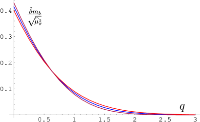
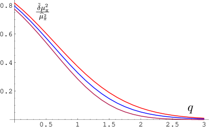
Figure 1: The dimensionless ratios $\tilde{\delta}m_{b}/(\widehat{\mu_{\pi}^{2}})^{\frac{1}{2}}$ and $\tilde{\delta}\mu_{\pi}^{2}/\widehat{\mu_{\pi}^{2}}$ as functions of the cut scale variable $q\!=\!\hat{Q}/(\widehat{\mu_{\pi}^{2}})^{\frac{1}{2}}$ as described in the text. The middle blue curve gives the central value, the average of the biases obtained using the two distribution functions.

3.2 Biases and perturbative corrections

The above bias evaluation was based purely on the nonperturbative primordial distribution. In reality cuts are applied to the observable spectrum resulting from the convolution of the perturbative and the nonperturbative pieces. Perturbative corrections modify the bias. Moreover, the effect of the perturbative corrections depends on their implementation, in particular on the separation scale $\mu$. Indeed, the moments of the combined spectrum are $\mu$-independent at a given cut, as it has to be for an observable. The biases computed with the nonperturbative distribution alone, on the other hand, would depend on the choice of $\mu$ since the distribution function and, in particular $m_{b}$ depend on the normalization scale.

It has been observed [5] that with the prototype Wilsonian perturbative spectrum of Ref. [21] perturbative contributions had little impact on the biases. Having calculated the perturbative spectrum explicitly with the Wilsonian cutoff, in this paper we adopt a more accurate direct approach. Namely, we determine the complete spectrum starting from this Wilsonian perturbative kernel. Simultaneously, we confront the results with the corresponding OPE predictions which include complete expressions for the perturbative moments derived from this spectrum, see Appendix A.1.

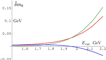
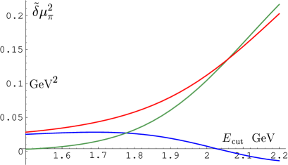
Figure 2: The perturbative effects on the biases $\tilde{\delta}m_{b}$ and $\tilde{\delta}\mu_{\pi}^{2}$. The red curve is the complete bias using the full spectrum. The green curve is the bias calculated without perturbative corrections, and the blue line shows the difference between the two curves.

Again we find that for $\mu\!\sim\!1\,\mbox{GeV}$ the biases are only weakly modified by the perturbative corrections. This is illustrated by Figs. 2, where we have assumed $m_{b}(1\,\mbox{GeV})\!=\!4.6\,\mbox{GeV}$ and $\mu_{\pi}^{2}(1\,\mbox{GeV})\!=\!0.45\,\mbox{GeV}^{2}$. Even so in our analysis we retain the perturbative shifts for the sake of completeness. At the same time, due to their smallish size we just approximate these shifts in $\tilde{\delta}m_{b}$ and in $\tilde{\delta}\mu_{\pi}^{2}$ by functions of only the single variable $q$, obtained at the central values expected for the parameters:

$$\Delta^{\rm pert}f_{s}(q)\mbox{~{}} \simeq \mbox{~{}}0.0103\,q^{3}\!-\!0.0729\,q^{2}\!+\!0.165\,q\!-\!0.111$$

$$\Delta^{\rm pert}g_{s}(q)\mbox{~{}} \simeq \mbox{~{}}-0.0138\,q^{3}\!+\!0.0.0437\,q^{2}\!+\!0.0316\,q\!-\!0.042\qquad$$ (16)

If necessary, these can be calculated anew at the final fitted values; the procedure converges well since the shifts are small.

3.3 Procedure

Let us summarize now the proposed way to obtain the numerical theory predictions for the photon energy moments. The inputs are the (true) values of the heavy quark parameters; they are assumed to be normalized at $\mu\!=\!1\,\mbox{GeV}$. The procedure consists of three steps. First, the ‘biased’, i.e. uncorrected moments are evaluated by adding the nonperturbative and perturbative contributions. The former are given by Eqs. (8), (9). The perturbative ones are described in detail in Appendix A.1; they refine the previously applied Eqs. (5). The first-order integrals $a_{k}$ are given in Eqs. (LABEL:231) and (LABEL:232) with $B_{1}$ defined in Eq. (A.2). The similar BLM pieces of the moments, $b_{k}$, are obtained by integrating Eq. (A.1) (and, for $b_{1}$, additionally subtracting the value of $B_{2}$ given by Eq. (A.22)). Alternatively, one can use the approximate numerical interpolations Eqs. (A.1) and (A.1).

Next with $\widehat{m_{b}}$ and $\widehat{\mu_{\pi}^{2}}$ defined in Eq.(12) we can determine the biases $\tilde{\delta}m_{b}$ and $\tilde{\delta}\mu_{\pi}^{2}$ using Eq. (14):

$$\tilde{\delta}m_{b}=\sqrt{\widehat{\mu_{\pi}^{2}}}\,f_{s}(q)\,,\qquad\tilde{\delta}\mu_{\pi}^{2}=\widehat{\mu_{\pi}^{2}}\,g_{s}(q)$$ (17)

with the dimensionless scaling variable $q=\!\hat{Q}/\sqrt{\widehat{\mu_{\pi}^{2}}}\,$, where $\hat{Q}\!=\!\widehat{m_{b}}\!-\!2E_{\rm cut}$.

Finally, we may apply additional small adjustments accounting for the perturbative impact on the biases. While obtained in a lengthy way using complicated expressions, they can be approximated quite adequately by simple polynomials as in Eqs. (16). To account for these effects one would replace, at the previous step

$$f_{s}(q)\Longrightarrow f_{s}(q)+\Delta^{\rm pert}f_{s}(q),\qquad g_{s}(q)\Longrightarrow g_{s}(q)+\Delta^{\rm pert}g_{s}(q)\;.$$ (18)

The thus corrected photon energy moments can then be confronted with the data.

Here we illustrate the procedure using the central values of the heavy quark parameters [24] very close to those reported by BaBar [2]:

$$m_{b}(1\,\mbox{GeV})\mbox{~{}} = \mbox{~{}}4.61\,\mbox{GeV},\qquad\mu_{\pi}^{2}(1\,\mbox{GeV})=0.41\,\mbox{GeV}^{2}$$ (19)

$$\rho_{D}^{3}(1\,\mbox{GeV})\mbox{~{}} = \mbox{~{}}0.17\,\mbox{GeV}^{3}.$$ (20)

Likewise we use the central number for the chromomagnetic value inferred from the $B^{*}-B$ mass difference, and we fix the one for the $LS$ term to its theoretical expectation:

$$\mu_{G}^{2}(1\,\mbox{GeV})=0.35\,\mbox{GeV}^{2},\qquad\rho_{LS}^{3}=-0.15\,\mbox{GeV}^{3}\;.$$ (21)

For $E_{\rm cut}\!=\!2.0\,\mbox{GeV}$ we have $x\!=\!0.8677$ and for the perturbative contributions we find from Eqs. (LABEL:231), (LABEL:232), (A.20)–(A.22) and (A.26):

$$a_{1}(0.8677;\mbox{$\frac{1}{4.61}$})+\hat{a}_{1}(0.8677)=-0.0511\,, b_{1}(0.8677;\mbox{$\frac{1}{4.61}$})+\hat{b}_{1}(0.8677)=-0.0909$$

$$a_{2}(0.8677;\mbox{$\frac{1}{4.61}$})+\hat{a}_{2}(0.8677)=\mbox{~{}}0.00447\,, b_{2}(0.8677;\mbox{$\frac{1}{4.61}$})+\hat{b}_{2}(0.8677)=0.00538\,;\qquad$$ (22)

using $\alpha_{s}\!=\!0.22$ and $\beta_{0}\!=\!9$ yields

$$\langle E_{\gamma}\rangle^{\rm pert}|_{E_{\gamma}>2.0\,{\rm GeV}}=2.328\,\mbox{GeV},\qquad\langle E_{\gamma}^{2}\!-\!\langle E_{\gamma}\rangle^{2}\rangle^{\rm pert}|_{E_{\gamma}>2.0\,{\rm GeV}}=0.00390\,\mbox{GeV}^{2}.$$ (23)

The nonperturbative power corrections given by Eqs. (8) and (9) are

$$\langle E_{\gamma}\rangle^{\rm power}=-0.00715\,\mbox{GeV},\qquad\langle E_{\gamma}^{2}\!-\!\langle E_{\gamma}\rangle^{2}\rangle^{\rm power}=0.0253\,\mbox{GeV}^{2}.$$ (24)

Adding the perturbative corrections and these power corrections results in

$$\langle E_{\gamma}\rangle|_{2.0\,{\rm GeV}}^{\rm biased}=\,2.321\,\mbox{GeV}\,,\qquad\langle(E_{\gamma}\!-\!\langle E_{\gamma}\rangle)^{2}\rangle|_{2.0\,{\rm GeV}}^{\rm biased}=\,0.0292\,\mbox{GeV}^{2}\;.$$ (25)

The last step is to correct for the biases. For our set of parameters, Eqs. (12) yield $\widehat{m_{b}}\!=\!4.602\,\mbox{GeV}$ or $\widehat{\Lambda}\!=\!0.677\,\mbox{GeV}$ and, using $r_{3}\!=\!0.75$, we obtain $\widehat{\mu_{\pi}^{2}}\!=\!0.330\,\mbox{GeV}^{2}$. At $E_{\rm cut}\!=\!2.0\,\mbox{GeV}$ the value of the effective normalized hardness is then $q\!=\!\hat{Q}/\sqrt{\widehat{\mu_{\pi}^{2}}}\!\simeq\!1.05$ and we have $r\!=\!\widehat{\mu_{\pi}^{2}}/\widehat{\Lambda}^{2}\!\simeq\!0.72$. We take the scaling form Eqs. (17) for the biases parametrized in Eqs. (15), and apply the shifts Eqs. (16) due to the perturbative effects according to Eqs. (18):

$$\tilde{\delta}m_{b}\mbox{~{}} = \mbox{~{}}\sqrt{\widehat{\mu_{\pi}^{2}}}\left(\,f_{s}(q)+\Delta^{\rm pert}f_{s}(q)\right)=0.041\,\mbox{GeV}$$

$$\tilde{\delta}\mu_{\pi}^{2}\mbox{~{}} = \mbox{~{}}\widehat{\mu_{\pi}^{2}}\left(\,g_{s}(q)+\Delta^{\rm pert}g_{s}(q)\right)=0.111\,\mbox{GeV}^{2}\;.$$ (26)

We arrive at the final bias-corrected values of the moments combining Eqs. (25) and (26) according to Eqs. (10):

$$\langle E_{\gamma}\rangle|_{2.0\,{\rm GeV}}\mbox{~{}} = \mbox{~{}}\langle E_{\gamma}\rangle|_{2.0\,{\rm GeV}}^{\rm biased}+\mbox{$\frac{\tilde{\delta}m_{b}}{2}$}=2.342\,\mbox{GeV}$$

$$\langle(E_{\gamma}\!-\!\langle E_{\gamma}\rangle)^{2}\rangle|_{2.0\,{\rm GeV}}\mbox{~{}} = \mbox{~{}}\langle(E_{\gamma}\!-\!\langle E_{\gamma}\rangle)^{2}\rangle|_{2.0\,{\rm GeV}}^{\rm biased}-\mbox{$\frac{\tilde{\delta}\mu_{\pi}^{2}}{12}$}=0.020\,\mbox{GeV}^{2}\;.$$ (27)

If we follow the similar procedure for other cuts, we find, for the biased average photon energy and the variance, the following values for $E_{\rm cut}\!=\!1.8$, $1.9$, $2.0$ and $2.1\,\mbox{GeV}$:

$$\langle E_{\gamma}\rangle|_{1.8\,{\rm GeV}}^{\rm biased}\mbox{~{}} \simeq \mbox{~{}}2.305\,\mbox{GeV}\qquad\qquad\langle(E_{\gamma}\!-\!\langle E_{\gamma}\rangle)^{2}\rangle|_{1.8\,{\rm GeV}}^{\rm biased}\simeq 0.0357\,\mbox{GeV}^{2}$$

$$\langle E_{\gamma}\rangle|_{1.9\,{\rm GeV}}^{\rm biased}\mbox{~{}} \simeq \mbox{~{}}2.313\,\mbox{GeV}\qquad\qquad\langle(E_{\gamma}\!-\!\langle E_{\gamma}\rangle)^{2}\rangle|_{1.9\,{\rm GeV}}^{\rm biased}\simeq 0.0321\,\mbox{GeV}^{2}$$

$$\langle E_{\gamma}\rangle|_{2.0\,{\rm GeV}}^{\rm biased}\mbox{~{}} \simeq \mbox{~{}}2.321\,\mbox{GeV}\qquad\qquad\langle(E_{\gamma}\!-\!\langle E_{\gamma}\rangle)^{2}\rangle|_{2.0\,{\rm GeV}}^{\rm biased}\simeq 0.0293\,\mbox{GeV}^{2}$$

$$\langle E_{\gamma}\rangle|_{2.1\,{\rm GeV}}^{\rm biased}\mbox{~{}} \simeq \mbox{~{}}2.329\,\mbox{GeV}\qquad\qquad\langle(E_{\gamma}\!-\!\langle E_{\gamma}\rangle)^{2}\rangle|_{2.0\,{\rm GeV}}^{\rm biased}\simeq 0.0271\,\mbox{GeV}^{2}\;.$$ (28)

The bias corrections read

$$\tilde{\delta}m_{b}|_{1.8\,{\rm GeV}}\mbox{~{}} \simeq \mbox{~{}}0.015\,\mbox{GeV}\,\qquad\qquad\tilde{\delta}\mu_{\pi}^{2}|_{1.8\,{\rm GeV}}\simeq 0.0574\,\mbox{GeV}^{2}$$

$$\tilde{\delta}m_{b}|_{1.9\,{\rm GeV}}\mbox{~{}} \simeq \mbox{~{}}0.024\,\mbox{GeV}\,\qquad\qquad\tilde{\delta}\mu_{\pi}^{2}|_{1.9\,{\rm GeV}}\simeq 0.0790\,\mbox{GeV}^{2}$$

$$\tilde{\delta}m_{b}|_{2.0\,{\rm GeV}}\mbox{~{}} \simeq \mbox{~{}}0.041\,\mbox{GeV}\,\qquad\qquad\tilde{\delta}\mu_{\pi}^{2}|_{2.0\,{\rm GeV}}\simeq 0.111\,\mbox{GeV}^{2}$$

$$\tilde{\delta}m_{b}|_{2.1\,{\rm GeV}}\mbox{~{}} \simeq \mbox{~{}}0.070\,\mbox{GeV}\,\qquad\qquad\tilde{\delta}\mu_{\pi}^{2}|_{2.1\,{\rm GeV}}\simeq 0.152\,\mbox{GeV}^{2}.\qquad$$ (29)

Then we arrive at the following final, i.e. bias-corrected predictions for the average and variance,

$$\langle E_{\gamma}\rangle|_{1.8\,{\rm GeV}}\mbox{~{}} \simeq \mbox{~{}}2.312\,\mbox{GeV},\qquad\qquad\langle(E_{\gamma}\!-\!\langle E_{\gamma}\rangle)^{2}\rangle|_{1.8\,{\rm GeV}}\simeq 0.0309\,\mbox{GeV}^{2}$$

$$\langle E_{\gamma}\rangle|_{1.9\,{\rm GeV}}\mbox{~{}} \simeq \mbox{~{}}2.325\,\mbox{GeV},\qquad\qquad\langle(E_{\gamma}\!-\!\langle E_{\gamma}\rangle)^{2}\rangle|_{1.9\,{\rm GeV}}\simeq 0.0255\,\mbox{GeV}^{2}$$

$$\langle E_{\gamma}\rangle|_{2.0\,{\rm GeV}}\mbox{~{}} \simeq \mbox{~{}}2.342\,\mbox{GeV},\qquad\qquad\langle(E_{\gamma}\!-\!\langle E_{\gamma}\rangle)^{2}\rangle|_{2.0\,{\rm GeV}}\simeq 0.020\,\mbox{GeV}^{2}$$

$$\langle E_{\gamma}\rangle|_{2.1\,{\rm GeV}}\mbox{~{}} \simeq \mbox{~{}}2.364\,\mbox{GeV},\qquad\qquad\langle(E_{\gamma}\!-\!\langle E_{\gamma}\rangle)^{2}\rangle|_{2.1\,{\rm GeV}}\simeq 0.0145\,\mbox{GeV}^{2}.$$ (30)

These numbers, in principle, can be compared with some published measurements (a more detailed analysis of the BELLE data has also been performed  ):

$$\langle E_{\gamma}\rangle|_{1.8\,{\rm GeV}}\mbox{~{}} \simeq \mbox{~{}}2.292\pm 0.026\pm 0.034\;\,\mbox{GeV}\;\;\;\mbox{\hskip 27.59915pt~{}}\mbox{BELLE }\cite[cite]{[\@@bibref{}{BELLE}{}{}]}$$

$$\langle(E_{\gamma}\!-\!\langle E_{\gamma}\rangle)^{2}\rangle|_{1.8\,{\rm GeV}}\mbox{~{}} \simeq \mbox{~{}}0.0305\pm 0.0074\pm 0.0063\;(\,\mbox{GeV})^{2}\;\;\;\mbox{BELLE }\cite[cite]{[\@@bibref{}{BELLE}{}{}]}$$

$$\langle E_{\gamma}\rangle|_{2.0\,{\rm GeV}}\mbox{~{}} \simeq \mbox{~{}}2.346\pm 0.032\pm 0.011\;\,\mbox{GeV}\;\;\;\mbox{\hskip 33.85875pt~{}}\mbox{CLEO }\cite[cite]{[\@@bibref{}{CLEO}{}{}]}$$

$$\langle(E_{\gamma}\!-\!\langle E_{\gamma}\rangle)^{2}\rangle|_{2.0\,{\rm GeV}}\mbox{~{}} \simeq \mbox{~{}}0.0226\pm 0.0066\pm 0.0020\;(\,\mbox{GeV})^{2}\;\;\;\mbox{\hskip 2.56073pt~{}}\mbox{CLEO }\cite[cite]{[\@@bibref{}{CLEO}{}{}]}$$ (31)

In view of the uncertainties in the experimental numbers and their high correlations we refrain from detailed comparison; yet there appears a clear trend that the bias corrections bring the predictions into close agreement with the data, in particular for the variance.

We want to emphasize the following features in the estimated values for biases:

• The biases increase steeply with the energy cuts.

• While for $E_{\rm cut}\!=\!1.8\,\mbox{GeV}$ they are rather insignificant, for $E_{\rm cut}\!\geq\!2.0\,\mbox{GeV}$ they become comparable to or even larger than the accuracy with which the corresponding parameters have been be extracted from $B\!\to\!X_{c}\,\ell\nu$.

• The uncertainties inherent in the evaluation of biases remain rather small for $m_{b}$, and even for $\mu_{\pi}^{2}$ they are of moderate size.

4 Effect of the four-quark operators at order $\alpha_{s}/m_{b}^{3}$

As noted previously [17, 27, 21], four-quark operators $(\bar{b}\Gamma_{i}s)\,(\bar{s}\Gamma_{i}b)$ do not contribute to $b\!\to\!s\!+\!\gamma$ at tree level, unlike for $b\!\to\!u\,\ell\nu$. Yet hard gluon emission induces Wilson coefficients for them already at order $\alpha_{s}$. Here we give their contributions. Similar short-distance corrections affect, in general, Wilson coefficients of all other operators, including those determining the moments of the light-cone distribution function. The four-quark effects, however are usually numerically enhanced, at least where they are allowed at the tree level.

To order $\alpha_{s}$ the effect is expressed in terms of two expectation values

$$S_{V}\mbox{~{}} = \mbox{~{}}(\delta_{ik}\delta_{lj}\!-\!\mbox{$\frac{1}{3}$}\delta_{ij}\delta_{lk})\frac{1}{2M_{B}}\,\langle B|\bar{b}^{i}\gamma_{\mu}b^{k}\,\bar{s}^{l}\gamma^{\mu}s^{j}|B\rangle$$

$$S_{A}\mbox{~{}} = \mbox{~{}}(\delta_{ik}\delta_{lj}\!-\!\mbox{$\frac{1}{3}$}\delta_{ij}\delta_{lk})\frac{1}{2M_{B}}\,\langle B|\bar{b}^{i}\gamma_{\mu}\gamma_{5}b^{k}\bar{s}^{l}\gamma^{\mu}\gamma_{5}s^{j}|B\rangle\;,$$ (32)

where the $i,j,k,l$ denote color indices, and yields the following contributions to the first three moments:

$$\Delta_{\bar{s}s}\langle(E_{\gamma}\!-\!\langle E_{\gamma}\rangle)^{2}\rangle\mbox{~{}} = \mbox{~{}}\!\!-\frac{\pi\alpha_{s}}{4}\left(\frac{S_{V}}{m_{b}}-\frac{1}{3}\frac{S_{A}}{m_{b}}\right)$$

$$\Delta_{\bar{s}s}\langle E_{\gamma}\rangle\mbox{~{}} = \mbox{~{}}\;\;\;\frac{\pi\alpha_{s}}{2}\left(-\frac{S_{V}}{m_{b}^{2}}+3\frac{S_{A}}{m_{b}^{2}}\right)$$

$$\frac{1}{\Gamma_{B\to X\gamma}}\Delta_{\bar{s}s}\Gamma_{B\to X\gamma}\mbox{~{}} = \mbox{~{}}\;\;\;2\pi\alpha_{s}\left(\frac{S_{V}}{m_{b}^{3}}+\frac{11}{3}\frac{S_{A}}{m_{b}^{3}}\right)\;;$$ (33)

the appropriate value of $\alpha_{s}$ here is about $0.3$. $S_{V,A}$ are related to the non-valence four-quark parameters $\omega_{V,A}$, $\tau_{V,A}$ of Ref. [28] through

$$S_{V}=\mbox{$\frac{8}{9}$}\omega_{V}-\mbox{$\frac{2}{3}$}\tau_{V}\,,\qquad S_{A}=\mbox{$\frac{8}{9}$}\omega_{A}-\mbox{$\frac{2}{3}$}\tau_{A}\;.$$ (34)

It should be noted that the contributions from the four-quark operators are $1/m_{b}^{3}$-suppressed only in the total width. In the higher moments an enhancement arises over naive expectations one might infer considering the fact that the four-quark operators contribute to the spectrum only in the end-point region where $E_{\gamma}\!-\!\frac{m_{b}}{2}\!\sim\!\mu_{\rm hadr}$, and that their overall effect on the width is $1/m_{b}^{3}$. The diagrams with a gluon exchanged between the light quark legs generate additional powers of $\epsilon\!=\!m_{b}\!-\!2E_{\gamma}$ in the denominator in the forward scattering amplitude; this directly affects the higher moments, but not the total rate. Accordingly, we find the corrections to the rate negligible, yet not necessarily so for $\langle E_{\gamma}\rangle$ and, in particular, for the second moment determining $\mu_{\pi}^{2}$. Since contributions from $(\bar{b}\Gamma_{i}s)(\bar{s}\Gamma_{i}b)$ can arise only via non-valence configurations in the $B$ meson (for the KM favored modes), they must be somewhat suppressed; yet the degree of suppression is uncertain.

The impact on the second moment and, therefore the related shift in the apparent value of $\mu_{\pi}^{2}$ could a priori be significant – if the generic non-valence ‘color-straight’ operators (in the terminology of Ref. [28]) are estimated through the vacuum chiral condensate $\langle\bar{s}s\rangle_{0}$ according to

$$\frac{1}{2M_{B}}\,\langle B|\bar{b}^{i}b^{i}\,\bar{s}^{k}s^{k}(0)|B\rangle\sim\frac{1}{2M_{B}}\,\langle B|\bar{b}^{i}b^{i}(0)|B\rangle\,\langle\bar{s}s\rangle_{0}\simeq-(200\,\mbox{MeV})^{3}\;.$$ (35)

A dedicated discussion of the non-factorizable four-fermion expectation values can be found in Ref. [28]. It turns out, though that the value of $S_{V}$ is expected to be particularly suppressed compared to the estimate (35). $S_{V}$, to leading order in $1/N_{c}$, reduces to the color-straight vector operator, non-valence expectation values for which (giving the $s$-quark number density at the origin) are probably small, since the density must vanish identically when integrated over the whole volume. The $1/N_{c}$ color-octet piece of $S_{V}$ contributing to the Darwin expectation value $\rho_{D}^{3}$, is probably larger, yet still suppressed.

A larger value is expected for the spin-dependent axial matrix element $S_{A}$, for which Eq. (35) can be conservatively taken as an upper bound. Yet the coefficient for $S_{A}$ is appreciable only in $\langle E_{\gamma}\rangle$ and in the total width where the effects are $1/m_{b}^{2}$- and $1/m_{b}^{3}$-suppressed, respectively. Therefore we think that the related corrections in $\langle E_{\gamma}\rangle$ are below $10\,\mbox{MeV}$ in $m_{b}$ and safely at the sub-percent level for the total width.

5 Cut-related uncertainties in $\;b\!\to\!c\,\ell\nu$

Lower cuts imposed on the charged lepton energy in $B\!\to\!X_{c}\,\ell\nu$ decays likewise degrade the hardness of the transition. Yet the final state in $b\to c\ell\nu$ exhibits kinematics more complex than in $b\to s+\gamma$, which makes this effect less transparent. Furthermore the dynamics is considerably more complicated as well, since the relevant distribution describing the dependence on the charged lepton energy cut, generally is neither the light-cone distribution nor the temporal distribution describing the effects of the ‘Fermi motion’ in the small velocity (SV) kinematics. There is no reason to expect an analogous distribution to be universal for different moments; the power corrections are probably significant in the realistic settings, and probably vary depending on the moments as well.

Nevertheless there are some common features between $B\!\to\!X_{s}+\gamma$ and $B\!\to\!X_{c}\,\ell\nu$, in particular due to the conceptual similarity of the OPE treatment of both cases. Furthermore the full impact of the degraded hardness might not reveal itself in the few lowest terms in the $1/m_{b}$ and $\alpha_{s}$ expansion that one is, in practice, limited to in the theoretical description.

As argued in Ref. [5], in this situation it is reasonable to adopt a cautious approach and use the bias estimates for $B\!\to\!X_{s}+\gamma$ merely to assess the potential magnitude of additional cut-related uncertainties in the theoretical predictions for the $b\!\to\!c\,\ell\nu$ transitions. Namely, the conventional OPE predictions for a particular moment, with or without the cut, depend on the heavy quark parameters. Assigning a cut-induced ’uncertainty’ to the values of those parameters (even though they have definite values in actual QCD), would result in an additional variation in the theoretical predictions, which can be used as an estimate of the scale of possible cut-related exponential pieces.

To implement this prescription in practice, we need a commensurate definition for the hardness in both transitions and how that scale is degraded by energy cuts. We advocate the following ansatz which is more accurate at low hardness:

$${\cal Q}_{\gamma}\simeq M_{B}\!-\!E_{\rm cut}^{\gamma}\!-\!\sqrt{(E^{\gamma}_{\rm cut})^{2}+M_{K^{*}}^{2}}\qquad\mbox{\sf vs.}\qquad{\cal Q}_{\rm sl}\simeq M_{B}\!-\!E_{\rm cut}^{\ell}\!-\!\sqrt{(E^{\ell}_{\rm cut})^{2}+M_{D^{*}}^{2}}\;;$$ (36)

equating the two yields the prescription

$$E_{\rm cut}^{\gamma}\Longleftrightarrow E_{\rm cut}^{\rm sl}+\frac{M_{D^{*}}^{2}-M_{K^{*}}^{2}}{2(E_{\rm cut}^{\rm sl}\!+\!\sqrt{(E^{\rm sl}_{\rm cut})^{2}\!+\!M_{D^{*}}^{2}})}\;.$$ (37)

for identifying equivalent energies in radiative and semileptonic decays. The resulting dependence is practically linear, Fig. 3.

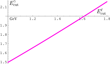
Figure 3: Cuts in $B\!\to\!X_{s}\!+\!\gamma\,$ and in $B\!\to\!X_{c}\,\ell\nu\,$ yielding the same overall hardness ${\cal Q}$

For a given $E_{\rm cut}^{\rm sl}$ we use Eq. (37) to determine the corresponding $E_{\rm cut}^{\gamma}$. This allows us to estimate the size of biases associated with $m_{b}$, $\mu_{\pi}^{2}$, $\rho_{D}^{3}$, … at this hardness. Using the explicit dependence of the semileptonic moments in question on these heavy quark parameters, one can estimate the degree to which the theoretical accuracy deteriorates due to the insufficient energy release. It is interesting to note that Refs. [29] concluded that when the lepton cut is raised to $1.7\,\mbox{GeV}$ theory looses control over $\langle M_{X}^{2}\rangle$. According to Fig. 3 the lepton cut at $1.7\,\mbox{GeV}$ corresponds to the cut on $E_{\gamma}$ at about $2.1\,\mbox{GeV}$ – and this is just the limit where the OPE for $B\!\to\!X_{s}\!+\!\gamma$ totally breaks down, according to the present estimates.

A possible physical motivation behind this procedure has been mentioned in Ref. [5]: the lower cuts both on $E_{\gamma}$ or on $E_{\ell}$ kinematically reduce or even eliminate the contribution of high mass hadronic final states in the decay, thus introducing an effective ‘normalization scale’ $\mu\!\approx\!{\cal Q}$. By virtue of the heavy quark sum rules, the integrals of the inclusive decay probabilities yield the values of the nonperturbative heavy quark parameters, with the upper cutoff on the mass of the produced states playing the role of the normalization point for the operators [27]. For large enough values of the hardness, explicit perturbative corrections account for this scale dependence, yet the possible nonperturbative dependence at limited ${\cal Q}$ is missed. This ansatz can therefore be interpreted as accounting for a certain nonperturbative evolution of the heavy quark parameters at relatively low normalization point $\mu$, provided it is to some extent universal, similar to the universality of the perturbative $\mu$-dependence of a given nonperturbative expectation value at $\mu$ in the perturbative domain.

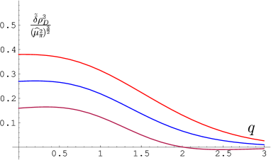
Figure 4: The expected bias for $\rho_{D}^{3}$: the dimensionless ratio $\tilde{\delta}\rho_{D}^{3}/(\widehat{\mu_{\pi}^{2}})^{\frac{3}{2}}$ for the two distribution functions and their average (blue)

For the sake of completeness we illustrate in Fig. 4 the expected size of the similar bias $\tilde{\rho}_{D}^{3}$ in the Darwin expectation value, which following Eqs. (10) is defined (up to a factor $-24$) as the cut-related deficit in the third moment of the photon spectrum. As anticipated, the predictions for the bias itself are less certain, yet we see that the corresponding effect can be significant down to rather low cuts.

6 Conclusions

In the present paper we addressed in detail the theoretical evaluation of the photon energy moments in $B\!\to\!X_{s}\!+\!\gamma$ decays with lower cuts on the photon energy, in terms of the underlying heavy quark parameters. These moments are particularly important in connection to the precision determination of the latter. Two general aspects have to be addressed in calculating the moments – perturbative contributions which act as corrections, and the nonperturbative effects dominating the measured low moments. We have improved the former by computing the perturbative spectrum with the explicit Wilsonian infrared cutoff on the low-energy gluon modes. This has been accomplished analytically including the BLM corrections.

We believe that this approach ensures the most accurate and trustworthy results for the heavy flavor decays with the heavy quark mass in a few GeV range, as it is for the actual beauty hadrons. Extensions of the method including resummation of the Sudakov radiation effects would be required for much heavier quarks, with masses exceeding $20\,\mbox{GeV}$.

Adding to what has been stated in Sect. 2.1, an essential element of the uncertainty in the numerical outcome of Refs. [14] is related to the unphysical, somewhat loose  shape function $S(\omega)$ arrived at in SCET in place of the truly Wilsonian $F(k_{+})$. Refs. [14] suggested that the properties of $S(\omega)$ required for constraining its possible form, may be related to the true Wilson heavy quark expectation values measured, say, in $B\!\to\!X_{c}\,\ell\nu$ decays. Yet in practice such relations suffer from poorly controlled perturbative corrections and seem too crude. It is unclear if their accuracy can realistically be improved. The advantage of employing the heavy quark distribution function $F(k_{+})$ is that its moments are directly related to the extracted expectation values; thus there is no significant uncertainty here.

Accordingly, we view our calculations of the spectrum and its moments as in all respects superior theoretically to the SCET-based evaluations of Refs. [14] and as more accurate numerically. This conclusion is illustrated, for instance, by Fig. 5 showing the perturbative (Wilsonian) photon spectrum (the $O_{7}$ part) in $b\!\to\!s\!+\!\gamma$.

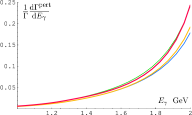
Figure 5: The significance of the higher-order BLM corrections in the Wilsonian perturbative spectrum ($\mu\!=\!1\,\mbox{GeV}$). Blue curve is the first-order spectrum evaluated with $\alpha_{s}\!=\!0.35$. Yellow curve is the usual $\alpha_{s}$ plus $\beta_{0}\alpha_{s}^{2}$ approximation, and the (barely visible) green line is obtained by adding the $\beta_{0}^{2}\alpha_{s}^{3}$ terms. Red curve shows the result of the full BLM resummation which can be performed precisely in the Wilsonian approach.

It suggests that the fraction of events with $E_{\gamma}\!<\!1.8\,\mbox{GeV}$ is not only small, but also reliably predicted, at least in what concerns the perturbative effects.

Doubts have been aired recently that the heavy-to-light transitions may not be treated with the conventional OPE, even abstracting from the complications associated with the high experimental cuts. In particular, the principal OPE results established more than a decade ago, were challenged. These results relate the moments of, say the photon energy spectrum to the local heavy quark expectation values which describe the nonperturbative bound-state dynamics. The OPE ensures universality – i.e. process-independence – of these expectation values as it should be for the characteristics of the initial bound state. Consequently, the same expectation values can be measured, say through the moments of the $B\!\to\!X_{c}\,\ell\nu$ distributions.

We find such agnostic claims unfounded. The recent paper [4] showed that, in spite of the well known peculiarities of the light-like jet processes associated with the collinear bremsstrahlung, the perturbative corrections to the moments of the photon spectrum are calculable in the usual short-distance expansion, without encountering new types of the nonperturbative effects. Our new perturbative calculations implement this idea in practice. We state that the photon moments can be precisely calculated in terms of the analogous expectation values determined from $B\!\to\!X_{c}\,\ell\nu$ moments, as long as the lower experimental cut on $E_{\gamma}$ is placed appropriately.

On the nonperturbative side the so-called bias effects due to significant lower cuts are in the focus of our study. They are missed in the routinely used simplified OPE expressions, yet turn out to be significant in practice. We showed that for actual $B$ decays these biases are affected very little by the perturbative corrections in the adequate Wilsonian approach with the separation scale chosen around the usual $1\,\mbox{GeV}$. This significantly simplifies incorporating the biases in practice.

The main phenomenological message can be expressed rather concisely:

• Imposing a lower cut on the photon energy in $B\!\to\!X_{s}+\gamma$ reduces the hardness ${\cal Q}$ of the transition.

• This impacts the evaluation of the energy moments in ways that are not fully described by the usual OPE expressions, thereby inducing systematic shifts, or biases.

• With the presently available accuracy of the measurements those biases can no longer be ignored.

• While those biases cannot be evaluated in a completely model-independent way yet, different ansätze for the heavy quark distribution functions, when constrained by the OPE, yield a consistent picture:

  • For $E_{\rm cut}^{\gamma}\!\lower 3.01385pt\hbox{$\;\stackrel{{\scriptstyle\textstyle<}}{{\sim}}\;$}\!1.7\,\mbox{GeV}$ they are more or less irrelevant.

  • For $E_{\rm cut}^{\gamma}\!>2.1\!\,\mbox{GeV}$ they are in all likelihood large, yet beyond accurate theoretical control.

  • In the range $1.8\,\mbox{GeV}\!\leq\!E_{\rm cut}^{\gamma}\!\leq\!2$ GeV they are significant, yet can be estimated with reasonable accuracy. Thus they can be corrected for.

• Lower cuts on the lepton energy in $B\!\to\!X_{c}\,\ell\nu$ conceptually have a similar impact on truncated lepton energy and hadronic mass moments. Yet the resulting biases in the values of the moments cannot be evaluated at present. We have suggested a simple prescription to obtain semi-quantitative estimates of the potential uncertainties associated with the high values of $E_{\rm cut}^{\ell}$.

We have presented the generally rather cumbersome theoretical evaluation of the truncated photon moments in a reasonably compact form suitable even for global fits of various data on inclusive $B$ decays. In our opinion, such data analyses must be done by experimentalists who can take care of numerous experimental subtleties. As the numerical application of our analysis, we only note that we find good agreement between the recently published BELLE data on the photon spectrum with the cut as low as $1.8\,\mbox{GeV}$, and the predictions based on the values of $m_{b}$, $\mu_{\pi}^{2}$ and $\rho_{D}^{3}$ extracted by BaBar from $B\!\to\!X_{c}\,\ell\nu$ [2]. The data and theory predictions coincide within $1\sigma$ of only the statistical error, cf. Eqs. (30) and (31), even without invoking other error bars or the uncertainties inherent in the theory calculations.

Acknowledgments: We are grateful to Th. Mannel for discussions and to our experimental colleagues U. Langenegger, V. Luth and in particular to O. Buchmueller for invaluable exchanges. Additional comments on the difference in our treatment with the SCET emerged after informative discussions with M. Neubert at the Belle Workshop and at KEK and his talks there, which are gratefully acknowledged. This work was supported in part by the NSF under grant number PHY-0087419.

Appendices

A.1 Perturbative spectrum with the Wilsonian scale separation

In Ref. [30] it has been described in detail how the required Wilsonian separation of soft and hard gauge field modes can be accomplished. The analysis of the semileptonic data based on this approach [31, 32] proved to be efficient and successful [2]. To order $\alpha_{s}$ it corresponds to a separation based on the energy $\omega\!=\!|\vec{k}\,|$ of the exchanged gluon: only those with $\omega\!>\!\mu$ are included into the Feynman integrals for the Wilson coefficients. While in higher orders the situation becomes considerably more involved, it can be handled for all BLM improvements similar to the first order case with only the relation between $\omega$ and $|\vec{k}\,|$ being modified.

Adopting this separation scheme one computes the usual one-gluon decay probability, yet with the extra factor $\theta(|\vec{k}\,|\!-\!\mu)$. A massless gluon in the decay necessarily has $|\vec{k}\,|\!<\!\frac{m_{b}}{2}$, hence taking $\mu\!>\!\frac{m_{b}}{2}$ would eliminate all bremsstrahlung. In what follows we will always assume $2\mu\!<\!m_{b}$; in practice, with $\mu$ around $1\,\mbox{GeV}$ we have $\frac{\mu}{m_{b}}\!\simeq\!0.22$. The integration over the thus restricted phase space is straightforward and yields

$$\frac{1}{\Gamma^{\rm pert}}\,\frac{{\rm d}\Gamma^{\rm pert}(\xi;\mu)}{{\rm d}\xi}=C_{F}\,\frac{\alpha_{s}}{\pi}\,f_{1}(\xi;\mbox{$\frac{\mu}{m_{b}}$})\,\theta(1\!-\!\xi)+A\,\delta(1\!-\!\xi)+C_{F}\,\frac{\alpha_{s}}{\pi}\,B_{1}\left(\mbox{$\frac{\mu}{m_{b}}$}\right)\delta^{\prime}(1\!-\!\xi)\;,$$ (A.1)

where the second term stands for the tree-level two-body decay modified by virtual corrections. Its strength $A$ is determined by the condition that the normalized spectrum in the l.h.s. integrated over the whole domain from $0\!\leq\!\xi\!\leq\!1$, is unity. The last term with $\delta^{\prime}(1\!-\!\xi)$ can be viewed as the reflection of the fact that the ‘kinetic’ mass $m_{b}(\mu)$ in the presence of perturbative corrections differs from the energy of the quark at rest (a ‘rest energy’ mass). The latter determines the perturbative end-point, in particular the photon energy in the two-body decay:

$$B_{1}(\eta)=\frac{4\,\eta}{3}\!+\!\frac{\eta^{2}}{2}\!-\!\frac{1}{2}\left(\ln{\left[\eta\!+\!\sqrt{1\!+\!\eta^{2}}\right]}\!+\!\eta\left(\sqrt{1+\eta^{2}}\!-\!\eta\right)\right)$$ (A.2)

The one-loop expression for the continuous part of the spectrum is

$$f_{1}(\xi;\eta)=\left\{\begin{array}[]{ll}\frac{2\,\xi^{3}\!-\!3\,\xi^{2}\!-\!6\,\xi\!}{4(1\!-\!\xi)}+\frac{\left(\xi^{2}\!-\!3\right)}{2(1\!-\!\xi)}\ln{(1\!-\!\xi)}&\qquad\xi\leq 1-2\eta\rule[-20.0pt]{0.0pt}{30.0pt}\\ \frac{(1\!-\!2\,\eta)\left(4\,\xi\,\eta^{2}\!-\!2\,\eta^{2}\!+\!4\,\xi^{2}\,\eta\!-\!6\,\xi\,\eta\!-\!\eta\!+\!2\,\xi\!-\!2\right)}{4\,\eta(1\!-\!\xi)}+\frac{\left(\xi^{2}\!-\!3\right)}{2(1\!-\!\xi)}\ln{(2\,\eta)}&\qquad\xi>1-2\eta\end{array}\right.$$ (A.3)

These allow to readily calculate the required moments of the perturbative spectrum:

$$\Phi_{0}(x;\eta)\mbox{~{}} = \mbox{~{}}\int_{x}^{1}\frac{1}{\Gamma^{\rm pert}}\,\frac{{\rm d}\Gamma^{\rm pert}(\xi;\mu)}{{\rm d}\xi}\;{\rm d}\xi\rule[-20.0pt]{0.0pt}{15.0pt}$$

$$= \mbox{~{}}\left\{\begin{array}[]{ll}\mbox{~{}}1-C_{F}\,\frac{\alpha_{s}}{\pi}\,\left[\frac{x\left(-2\,x^{2}\!+\!3\,x\!+\!30\right)}{12}+\frac{\left(-x^{2}\!-\!2\,x\!+\!10\right)}{4}\ln{(1\!-\!x)}\!+\!\frac{1}{2}\ln^{2}{(1\!-\!x)}\right]&\mbox{~{}}\mbox{for}\;x\!\leq\!1\!-\!2\eta\rule[0.0pt]{0.0pt}{20.0pt}\\ \mbox{~{}}1-C_{F}\,\frac{\alpha_{s}}{\pi}\left[\frac{1\!-\!2\,\eta}{12\eta}\left(-6\,\eta\,x^{2}\!-\!12\,\eta^{2}\,x\!+\!6\,\eta\,x\!-\!6\,x\!-\!8\,\eta^{3}\!+\!2\,\eta^{2}\!+\!19\,\eta\!+\!6\right)\right.&\rule[-10.0pt]{0.0pt}{40.0pt}\\ +\left.\frac{4\,\eta^{2}\!-\!8\,\eta\!+\!4\ln{(2\,\eta)}+\!3\!}{4}\ln{(1\!-\!x)}+\frac{-x^{2}\!-\!2\,x\!-\!4\eta^{2}\!+8\,\eta\!+\!7}{4}\ln{(2\,\eta)}-\frac{1}{2}\ln^{2}{(2\,\eta)}\right]&\mbox{~{}}\mbox{for}\;x\!>\!1\!-\!2\eta\\ \end{array}\right.$$

$$C_{F}\mbox{$\frac{\alpha_{s}}{\pi}$}\,a_{1}(x;\eta)\mbox{~{}} = \mbox{~{}}\int_{x}^{1}\frac{1}{\Gamma^{\rm pert}}\,\frac{{\rm d}\Gamma^{\rm pert}(\xi;\mu)}{{\rm d}\xi}(1\!-\!\xi)\,{\rm d}\xi\rule[-20.0pt]{0.0pt}{15.0pt}$$

$$= \mbox{~{}}\left\{\begin{array}[]{ll}\mbox{~{}}C_{F}\,\frac{\alpha_{s}}{\pi}\,\left[\frac{1}{72}\left(48\,\eta^{4}\!-\!64\,\eta^{3}\!+\!72\,\eta^{2}\!-\!72\,\eta\!-\!9\,x^{4}\!+\!22\,x^{3}\!+\!60\,x^{2}\!-\!96\,x\!+\!23\right)\right.\mbox{~{}}&\rule[-10.0pt]{0.0pt}{30.0pt}\\ \left.\mbox{\hskip 25.60747pt~{}}+\frac{(1-x)(x^{2}\!+\!x\!-\!8)}{6}\ln{(1\!-\!x)}-B_{1}(\eta)\right]&\mbox{~{}}\mbox{for}\;x\!\leq\!1\!-\!2\eta\rule[-5.0pt]{0.0pt}{10.0pt}\mbox{~{}}\\ \mbox{~{}}C_{F}\,\frac{\alpha_{s}}{\pi}\left[\frac{(1\!-\!x)(1\!-\!2\,\eta)}{12\,\eta}\left(4\,\eta\,x^{2}\!+\!6\,\eta^{2}\,x\!-\!5\,\eta\,x\!+\!3x\,\!-8\,\eta\!-\!3\right)\right.&\rule[15.0pt]{0.0pt}{10.0pt}\\ \left.\mbox{\hskip 25.60747pt~{}}\;+\frac{(1-x)(x^{2}\!+\!x\!-\!8)}{6}\ln{(2\,\eta)}-B_{1}(\eta)\right]&\mbox{~{}}\mbox{for}\;x\!\geq\!1\!-\!2\eta\mbox{~{}}\rule[10.0pt]{0.0pt}{10.0pt}\\ \end{array}\right.$$ (A.10)

$$C_{F}\mbox{$\frac{\alpha_{s}}{\pi}$}\,a_{2}(x;\eta)\mbox{~{}} = \mbox{~{}}\int_{x}^{1}\frac{1}{\Gamma^{\rm pert}}\,\frac{{\rm d}\Gamma^{\rm pert}(\xi;\mu)}{{\rm d}\xi}(1\!-\!\xi)^{2}\,{\rm d}\xi\rule[-15.0pt]{0.0pt}{25.0pt}$$

$$= \mbox{~{}}\left\{\begin{array}[]{ll}\mbox{~{}}C_{F}\,\frac{\alpha_{s}}{\pi}\,\left[\frac{1}{1440}\left(768\,\eta^{5}\!-\!720\,\eta^{4}\!+\!640\,\eta^{3}\!-\!480\,\eta^{2}\!+\!144\,x^{5}\!-\!495\,x^{4}\!-\!340\,x^{3}\!\right.\right.\mbox{~{}}&\rule[-10.0pt]{0.0pt}{20.0pt}\\ \mbox{\hskip 25.60747pt~{}}\left.\left.\;+1650\,x^{2}\!-\!1020\,x\!+\!61\right)\!+\!\frac{(1\!-\!x)^{2}(3\,x^{2}\!+\!2\,x\!-\!17)}{24}\ln{(1\!-\!x)}\right]&\mbox{~{}}\mbox{ for}\;x\!\leq\!1\!-\!2\eta\mbox{~{}}\\ \mbox{~{}}C_{F}\,\frac{\alpha_{s}}{\pi}\left[\frac{(1\!-\!x)^{2}(1\!-\!2\,\eta)}{24\,\eta}\left(6\,\eta\,x^{2}\!+\!8\,\eta^{2}\,x\!-\!8\,\eta\,x\!+\!4\,x\,\!-\!2\,\eta^{2}\!-\!7\,\eta\!-\!4\right)\right.&\rule[20.0pt]{0.0pt}{10.0pt}\\ \left.\mbox{\hskip 25.60747pt~{}}\;+\frac{(1\!-\!x)^{2}(3\,x^{2}\!+\!2\,x\!-\!17)}{24}\ln{(2\,\eta)}\right]&\mbox{~{}}\mbox{ for}\;x\!\geq\!1\!-\!2\eta\mbox{~{}}\rule[10.0pt]{0.0pt}{10.0pt}\\ \end{array}\right.$$ (A.15)

The usually considered BLM corrections can easily be calculated to arbitrary order with merely technical modifications. The corresponding technique has been reviewed in Refs. [33, 30]. First the one-gluon decay rate must be calculated with a non-vanishing fictitious gluon mass $m_{g}$ reflecting the gluon conversion into the $q\bar{q}$ or $gg$ pairs. This modifies the cutoff condition: $\theta(|\vec{k}\,|\!-\!\mu)$ is replaced by $\theta(\omega\!-\!\mu)=\theta(\vec{k}^{\,2}\!+\!m_{g}^{2}\!-\!\mu^{2})$. The integrals are still easily taken. All the functions additionally depend now on the new dimensionless parameter $\lambda\!\equiv\!\frac{m_{g}^{2}}{m_{b}^{2}}$ (note that in Ref. [30] this ratio was denoted by $\lambda^{2}$). Generalizing Eq. (A.1) we then set

$$\frac{1}{\Gamma^{\rm pert}}\,\frac{{\rm d}\Gamma^{\rm pert}(\xi,m_{g};\mu)}{{\rm d}\xi}=C_{F}\,\frac{\alpha_{s}}{\pi}\,f_{1}(\xi,\lambda;\eta)\,\theta(1\!-\!\xi\!-\!\lambda)+A\,\delta(1\!-\!\xi)+C_{F}\,\frac{\alpha_{s}}{\pi}\,B_{1}\left(\eta;\lambda\right)\delta^{\prime}(1\!-\!\xi)$$ (A.17)

(recall that $\eta\!<\!\frac{1}{2}$ is assumed; otherwise the kinematic constraints are modified), with

$$B_{1}\left(\mbox{$\eta$};\lambda\right)\mbox{~{}} = \mbox{~{}}\frac{4}{3}\sqrt{\eta^{2}\!-\!\lambda}\left(1\!-\!\mbox{$\frac{\lambda}{4\,\eta^{2}}$}\right)\!-\!\frac{\pi\sqrt{\lambda}}{2}\!+\!\sqrt{\lambda}\arcsin{\left(\mbox{$\frac{\sqrt{\lambda}}{\eta}$}\right)}\!+\!\frac{(\eta^{2}\!-\!\lambda)^{\frac{3}{2}}}{2\,\eta}$$

$$- \mbox{~{}}\frac{1}{4}\left(2\!-\!\lambda\right)\sqrt{\lambda\left(4\!-\!\lambda\right)}\left(\arctan{\left[\frac{(\lambda\!-\!2)\sqrt{\eta^{2}\!-\!\lambda}}{\sqrt{\lambda\left(4\!-\!\lambda\right)\left(\eta^{2}\!-\!\lambda+1\right)}}\right]}\!-\!\arctan{\left[\frac{\lambda\sqrt{\eta^{2}\!-\!\lambda}}{\eta\sqrt{\lambda\left(4\!-\!\lambda\right)}}\right]}\right)$$ (A.18)

$$- \mbox{~{}}\frac{1}{8}\lambda\left(4\!-\!\lambda\right)\left(2\,\ln{[\eta\!+\!\sqrt{\eta^{2}\!-\!\lambda}]}\!-\!\ln{\lambda}\right)\!-\!\frac{\lambda^{2}\!-\!4\lambda\!+\!2}{4}\ln{(\sqrt{\eta^{2}\!-\!\lambda\!+\!1}\!+\!\sqrt{\eta^{2}\!-\!\lambda})}$$

$$- \mbox{~{}}\frac{\sqrt{\eta^{2}\!-\!\lambda}}{2}\left(\sqrt{\eta^{2}\!-\!\lambda\!+\!1}\!-\!\eta\right).\qquad$$

To calculate the BLM corrections, we must integrate over the gluon mass. The upper end of the $\mu$-independent lower region of the spectrum now rises depending on $\lambda$: the perturbative spectrum is independent of $\mu$ if $\lambda\!>2\,\eta\,(1\!-\!\xi)\!-\!(1\!-\!\xi)^{2}$:

$$f_{1}\left(\xi;\mbox{$\eta$};\mbox{$\lambda$}\right)\mbox{~{}} = \mbox{~{}}\frac{\xi\,(\xi\!+\!\lambda\!-\!1)}{4(1\!-\!\xi)^{3}(\xi^{2}\!-\!2\,\xi\!+\!\xi\,\lambda\!+\!1)}\left(2\,\xi^{3}\lambda^{2}\!-\!3\,\xi^{2}\lambda^{2}\!+\!2\,\xi\lambda^{2}\!+\!4\,\xi^{4}\,\lambda\!-\!14\,\xi^{3}\lambda\!+\!17\,\xi^{2}\,\lambda\!-\!11\,\xi\lambda\!\right.\rule[-10.0pt]{0.0pt}{30.0pt}$$

  $$+\left.4\,\lambda\!+\!2\,\xi^{5}\!-\!9\,\xi^{4}\!+\!9\,\xi^{3}\!+\!7\,\xi^{2}\!-\!15\,\xi\!+\!6\right)\!+\!\frac{2\,\xi\,\lambda\!-\!2\,\lambda\!+\!\xi^{2}\!-\!3}{2(1\!-\!\xi)}\ln{\left(1\!-\!\xi\!+\!\frac{\xi\,\lambda}{1\!-\!\xi}\right)}$$

$$\mbox{\hskip 280.25964pt~{}}\mbox{at}\;\lambda\!\geq\!2\eta(1\!\!-\!\!\xi)\!\!-\!\!(1\!\!-\!\!\xi)^{2}\rule[-20.0pt]{0.0pt}{30.0pt}\vspace*{-50pt}$$

$$= \mbox{~{}}\frac{(2\,\eta\!-\!\lambda\!-\!1)}{4(1\!-\!\xi)^{2}(2\,\eta\!-\!\lambda)}\left(-2\,\xi^{2}\,\lambda^{2}\!+\!\xi\,\lambda^{2}\!-\!\lambda^{2}\!-\!4\,\xi^{3}\,\lambda\!+\!12\,\xi^{2}\,\lambda\!+\!4\,\eta\,\xi\,\lambda\!-\!9\,\xi\,\lambda\!+\!\lambda\!\right.\rule[-10.0pt]{0.0pt}{30.0pt}$$

$$\mbox{~{}}\left.+8\,\eta\,\xi^{3}\!+\!8\,\eta^{2}\,\xi^{2}\!-\!20\,\eta\,\xi^{2}\!+\!4\,\xi^{2}\!-\!12\,\eta^{2}\,\xi\!+\!10\,\eta\,\xi\!-\!8\,\xi\!+\!4\,\eta^{2}\!+\!2\,\eta\!+\!4\right)\rule[-10.0pt]{0.0pt}{30.0pt}$$

$$\mbox{~{}}+\frac{2\,\xi\,\lambda\!-\!2\,\lambda\!+\!\xi^{2}\!-\!3}{2(1\!-\!\xi)}\ln{\left(2\,\eta-\lambda\right)}\mbox{\hskip 142.26378pt~{}}\mbox{{ at $\lambda\!\leq\!2\eta(1\!\!-\!\!\xi)\!\!-\!\!(1\!\!-\!\!\xi)^{2}$}}$$

The above $\lambda$-dependent functions replace the usual one-loop ones of Eqs. (A.1)-(A.3). Using Eqs. (A.18), (LABEL:241) it is not difficult to obtain the BLM corrections both to the spectrum and to its moments. For instance, for the continuous part of the spectrum, at $\xi\!\leq\!1\!-\!2\eta$ we integrate the upper of the two expressions in Eq. (LABEL:241) over $\lambda$ directly from $\lambda\!=\!0$ to $\lambda\!=\!1\!-\!\xi$. At $\xi\!>\!1\!-\!2\eta$ the integral from $\lambda\!=\!0$ to $\lambda\!=\!(1\!-\!\xi)(\xi\!-\!1\!+\!2\eta)$ uses the lower expression, while the integrand in the integral from $\lambda\!=\!(1\!-\!\xi)(\xi\!-\!1\!+\!2\eta)$ to $\lambda\!=\!1-\!\xi$ is the $\eta$-independent upper expression. The subtraction piece employing $\lambda\!=\!0$, of course is integrated over $\lambda$ from $0$ to $\infty$,  cf. Eq. (A.22).

Representing the spectrum as

$$\frac{1}{\Gamma^{\rm pert}}\,\frac{{\rm d}\Gamma^{\rm pert}(\xi;\mu)}{{\rm d}\xi} \mbox{~{}}=\mbox{~{}} C_{F}\,\frac{\alpha_{s}}{\pi}\,\left[f_{1}(\xi;\mbox{$\frac{\mu}{m_{b}}$})+\beta_{0}\mbox{$\frac{\alpha_{s}}{\pi}$}\,f_{2}(\xi;\mbox{$\frac{\mu}{m_{b}}$})+...\;\right]\,\theta(1\!-\!\xi)+A\,\delta(1\!-\!\xi)+$$ (A.20)

$$\mbox{\hskip 28.45274pt~{}}C_{F}\,\frac{\alpha_{s}}{\pi}\,\left[B_{1}\left(\mbox{$\frac{\mu}{m_{b}}$}\right)+\beta_{0}\mbox{$\frac{\alpha_{s}}{\pi}$}B_{2}\left(\mbox{$\frac{\mu}{m_{b}}$}\right)+...\;\right]\,\delta^{\prime}(1\!-\!\xi)\;,\qquad$$

$f_{1}$ and $B_{1}$ are given in Eqs. (A.3) and (A.2), respectively, while for the second-order BLM parts we obtain:

$$f_{2}(\xi;\eta)\mbox{~{}} = \mbox{~{}}\frac{38\,\xi^{3}\!-\!93\,\xi^{2}\!+\!6\,\xi\!-\!36}{96(1\!-\!\xi)}-\frac{6\,\xi^{4}\!-\!31\,\xi^{3}\!+\!24\,\xi^{2}\!-\!30\,\xi\!+\!18}{48\,\xi(1\!-\!\xi)}\ln{(1\!-\!\xi)}\rule[-15.0pt]{0.0pt}{20.0pt}$$

$$-\frac{3(\xi^{2}\!-\!3)}{16(1\!-\!\xi)}\left(\ln^{2}{(1\!-\!\xi)}\!+\!\frac{2}{3}{\rm Li}_{2}(\xi)\right)\mbox{\hskip 193.19418pt~{}}\xi\!\leq\!1\!-\!2\eta\rule[-30.0pt]{0.0pt}{40.0pt}$$

$$= \mbox{~{}}\frac{6\,\eta\,\xi^{3}\!-\!(128\,\eta^{2}\!-\!16\,\eta)\xi^{2}\!-\!(128\,\eta^{3}\!-\!244\,\eta^{2}\!+\!52\,\eta\!-\!20)\xi+52\,\eta^{3}\!+\!12\,\eta^{2}\!-\!15\,\eta\,-\,20}{96\,\eta\,(1\!-\!\xi)}$$

$$\mbox{~{}}+\frac{(8\,\eta^{2}\!-\!4\,\eta)\,\xi^{2}\!+\!(8\,\eta^{3}\!-\!16\,\eta^{2}\!+\!10\,\eta-2)\,\xi\!-\!4\,\eta^{3}\!-\!3\,\eta\!+\!2}{16\,\eta\,(1\!-\!\xi)}\left(\ln{(1\!-\!\xi)}\!+\!\ln{(2\,\eta\!+\!\xi\!-\!1)}\right)\rule[-10.0pt]{0.0pt}{20.0pt}$$

$$\mbox{~{}}+\frac{2\,\xi^{3}\!-\!3\,\xi^{2}\!-\!6\,\xi}{16\,(1\,-\,\xi)}\ln{(2\,\eta\!+\!\xi\!-\!1)}+\frac{10\,\eta\,\xi^{2}\!-\!2\,(12\,\eta^{2}\!+\!3\,\eta\!+\!3)\,\xi\!+\!24\,\eta^{2}\!-\!24\,\eta\!+\!6}{48\,\eta\,(1\!-\!\xi)}\ln{(2\,\eta)}\rule[-10.0pt]{0.0pt}{20.0pt}$$

$$\mbox{~{}}+\frac{4\,\xi^{3}\,\eta\!+\!2(4\,\eta^{2}\!-\!6\,\eta\!+\!1)\xi^{2}\!-\!2(4\,\eta^{2}\!-\!9\,\eta\!+\!1)\,\xi\!-\!6\,\eta}{16\,\eta\,\xi(1\!-\!\xi)}\ln{(\xi^{2}\!+\!2\,\eta\,\xi\!-\!2\,\xi\!+\!1)}\rule[-10.0pt]{0.0pt}{20.0pt}$$

$$\mbox{~{}}+\frac{\left(\xi^{2}\!-\!3\right)}{8(1\!-\!\xi)}\left\{\vphantom{\frac{\xi\,(2\,\eta\!+\!\xi\!-\!1)}{\xi\!-\!1}}\ln{(1\!-\!\xi)}\ln{(2\,\eta\!+\!\xi\!-\!1)}\!-\!\ln{(1\!-\!\xi)}\ln{(2\,\eta)}\!-\!\ln{(2\,\eta)}\ln{(2\,\eta\!+\!\xi\!-\!1)}\right.\rule[-10.0pt]{0.0pt}{20.0pt}\mbox{~{}}$$

$$\left.\mbox{~{}}-\frac{1}{2}\ln^{2}{\!(1\!-\!\xi)}\!-\!{\rm Li}_{2}(\xi)\!+\!{\rm Li}_{2}\!\left(\!\frac{(1\!-\!\xi)(2\,\eta\!+\!\xi\!-\!1)}{2\,\eta}\right)\!-\!{\rm Li}_{2}\!\left(\!\frac{\xi\,(2\,\eta\!+\!\xi\!-\!1)}{\xi\!-\!1}\right)\right\}\mbox{\hskip 18.49428pt~{}}\xi\!>\!1\!-\!2\eta\mbox{~{}}$$

The BLM correction to the coefficient of the $\delta^{\prime}(1\!-\!\xi)$ can be obtained by numerically integrating over $\lambda$

$$B_{2}\left(\mbox{$\eta$}\right)=\frac{1}{4}\int_{0}^{\infty}\frac{d\lambda}{\lambda}\left(\frac{B_{1}\left(\mbox{$\eta$};\mbox{$0$}\right)}{1+e^{-5/3}\lambda}\!-\!B_{1}\left(\mbox{$\eta$};\mbox{$\lambda$}\right)\right)$$ (A.22)

The complete $\mu$-dependent analytic expressions for the BLM corrections to the moments contain polylog functions at worst, but are somewhat cumbersome, and we do not quote them here. At $\mu\!=\!0$ the order-$\alpha_{s}$ spectrum and its second-order BLM correction reproduce the standard expressions [13]

$$f_{1}(\xi;0) \mbox{~{}}=\mbox{~{}} \frac{2\,\xi^{3}\!-\!3\,\xi^{2}\!-\!6\,\xi\!}{4(1\!-\!\xi)}+\frac{\left(\xi^{2}\!-\!3\right)}{2(1\!-\!\xi)}\ln{(1\!-\!\xi)}$$ (A.23)

$$f_{2}(\xi;0) \mbox{~{}}=\mbox{~{}} \frac{38\,\xi^{3}\!-\!93\,\xi^{2}\!+\!6\,\xi\!-\!36}{96(1\!-\!\xi)}-\frac{6\,\xi^{4}\!-\!31\,\xi^{3}\!+\!24\,\xi^{2}\!-\!30\,\xi\!+\!18}{48\,\xi(1\!-\!\xi)}\ln{(1\!-\!\xi)}$$ (A.24)

$$\mbox{~{}}-\mbox{~{}} \frac{3(\xi^{2}\!-\!3)}{16(1\!-\!\xi)}\left(\ln^{2}{(1\!-\!\xi)}\!+\!\frac{2}{3}{\rm Li}_{2}(\xi)\right)\;.$$

Their moments, $\,a_{k}(x;0)\,$ and $\,b_{k}(x;0)$, respectively are given by

$$\int_{0}^{x}f_{1}(\xi;0)\;{\rm d}\xi \mbox{~{}}=\mbox{~{}} \frac{x\left(-2\,x^{2}\!+\!3\,x\!+\!30\right)}{12}+\frac{\left(-x^{2}\!-\!2\,x\!+\!10\right)}{4}\ln{(1\!-\!x)}\!+\!\frac{1}{2}\ln^{2}{(1\!-\!x)}$$

$$\int_{0}^{x}f_{2}(\xi;0)\;{\rm d}\xi \mbox{~{}}=\mbox{~{}} \frac{-14\,x^{3}\!+\!41\,x^{2}\!+\!120\,x\!-\!48\,\zeta(3)}{96}\!+\!\frac{1}{4}{\rm Li}_{2}\left(x\right)\ln{(1\!-\!x)}$$

$$\mbox{~{}}+\mbox{~{}} \frac{4\,x^{3}\!-\!31\,x^{2}\!-\!44\,x\!-\!8\,\pi^{2}\!+\!156}{96}\ln{(1\!-\!x)}\!+\!\frac{x^{2}\!+\!2\,x\!+\!6}{16}{\rm Li}_{2}\left(x\right)$$

$$\mbox{~{}}+\mbox{~{}} \frac{9\,x^{2}\!+\!18\,x\!-\!40\!+\!24\ln{(x)}}{96}\ln^{2}{(1\!-\!x)}\!-\!\frac{1}{8}\ln^{3}{(1\!-\!x)}\!+\!\frac{1}{2}{\rm Li}_{3}\left(1\!-\!x\right)$$

$$\int_{x}^{1}f_{1}(\xi;0)\;(1\!-\!\xi){\rm d}\xi \mbox{~{}}=\mbox{~{}} \frac{1}{72}\left(-\!9\,x^{4}\!+\!22\,x^{3}\!+\!60\,x^{2}\!-\!96\,x\!+\!23\right)\!+\!\frac{(1\!-\!x)(x^{2}\!+\!x\!-\!8)}{6}\ln{(1\!-\!x)}$$

$$\int_{x}^{1}f_{2}(\xi;0)\;(1\!-\!\xi){\rm d}\xi \mbox{~{}}=\mbox{~{}} \frac{408\,\pi^{2}\!-\!369\,x^{4}\!+\!1360\,x^{3}\!-\!66\,x^{2}\!+\!1380\,x\!-\!2305}{3456}\!+\!\frac{x^{3}\!-\!9\,x\!-\!9}{24}{\rm Li}_{2}\left(x\right)$$

$$\mbox{~{}}-\mbox{~{}} (1\!-\!x)\left(\frac{9\,x^{3}\!-\!61x\,^{2}\!-\!7\,x\!-\!7}{288}\ln{(1\!-\!x)}\!+\!\frac{x^{2}\!+\!x\!-\!8}{16}\ln^{2}{(1\!-\!x)}\right)$$

$$\int_{x}^{1}f_{1}(\xi;0)\;(1\!-\!\xi)^{2}{\rm d}\xi \mbox{~{}}=\mbox{~{}} \frac{1}{1440}\left(144\,x^{5}\!-\!495\,x^{4}\!-\!340\,x^{3}+1650\,x^{2}\!-\!1020\,x\!+\!61\right)$$

$$\mbox{~{}}+\mbox{~{}} \frac{(1\!-\!x)^{2}(3\,x^{2}\!+\!2\,x\!-\!17)}{24}\ln{(1\!-\!x)}$$

$$\int_{x}^{1}f_{2}(\xi;0)\;(1\!-\!\xi)^{2}{\rm d}\xi \mbox{~{}}=\mbox{~{}} \frac{7950\,\pi^{2}\!+\!7272\,x^{5}\!-\!33435x\,^{4}\!+\!35320\,x^{3}\!-\!25995\,x^{2}\!+\!91110\,x\!-\!74272}{86400}$$ (A.25)

$$\mbox{~{}}+\mbox{~{}} \frac{-3x\,^{4}\!+\!4\,x^{3}\!+\!18\,x^{2}\!-\!36\,x\!-\!36}{96}{\rm Li}_{2}\left(x\right)\!-\!\frac{(1\!-\!x)^{2}(3\,x^{2}\!+\!2\,x\!-\!17)}{48}\ln^{2}{(1\!-\!x)}$$

$$\mbox{~{}}+\mbox{~{}} \frac{(1\!-\!x)(72\,x^{4}\!-\!528\,x^{3}\!+\!562\,x^{2}\!-\!473\,x\!+\!1957)}{2880}\ln{(1\!-\!x)}$$

Finally, we provide simple numerical expressions for the first and second moments of the second order BLM correction with $\mu/m_{b}$ fixed at the value $1/4.6$:

$$b_{1}(x;\mbox{$\frac{1}{4.6}$})\!=\!\mbox{\hskip 398.33858pt~{}}$$

$$-B_{2}(\mbox{$\frac{1}{4.6}$})+\int_{x}^{1}\!\!f_{2}(\xi;\mbox{$\frac{1}{4.6}$})\;(1\!-\!\xi){\rm d}\xi=\left\{\begin{array}[]{ll}\!\!-0.032\!-\!0.096\,y\!-\!0.67\,y^{2}\!+\!1.6\,y^{3}\!-\!3.2\,y^{4}&\mbox{for }y\geq 0\rule[-10.0pt]{0.0pt}{10.0pt}\\ \!\!-0.032\!-\!0.11\,y\!-\!0.33\,y^{2}\!-\!0.47\,y^{3}\!-\!0.26\,y^{4}&\mbox{for }y\leq 0\end{array}\right.$$

$$\mbox{\hskip 56.9055pt~{}}y\equiv x-(1-2/4.6)$$

$$b_{2}(x;\mbox{$\frac{1}{4.6}$})\!=\!\int_{x}^{1}\!\!f_{2}(\xi;\mbox{$\frac{1}{4.6}$})\;(1\!-\!\xi)^{2}{\rm d}\xi=\left\{\begin{array}[]{ll}\!\!0.0225\!-\!0.051\,y\!-\!0.066\,y^{2}\!+\!0.040\,y^{3}\!+\!0.24\,y^{4}&\mbox{for }y\geq 0\rule[-10.0pt]{0.0pt}{10.0pt}\\ \!\!0.0225\!-\!0.050\,y\!-\!0.12\,y^{2}\!-\!0.12\,y^{3}\!-\!0.04\,y^{4}&\mbox{for }y\leq 0\end{array}\right.$$

They are sufficiently accurate in the whole relevant domain of $x$ between $0.65$ and $0.93$. The evaluation for different values of $m_{b}$ can easily be recovered from the fact that the above integrals are functions of the ratio $\mu/m_{b}$, and at fixed $m_{b}$ the $\mu$-dependence is well described by Eqs. (7).

A.2 Non-$O_{7}$ perturbative corrections

The non-$O_{7}$ spectrum was given in Ref. [13]. We have interpolated the moments of these contributions for $\frac{m_{c}}{m_{b}}\!=\!\frac{1.18}{4.61}$:

$$100\,\hat{a}_{1}(x)\mbox{~{}} = \mbox{~{}}\mbox{$\frac{C_{2}^{2}}{C_{7}^{2}}$}[0.053\!-\!0.81\,(x\!-\!0.87)+2.93\,(x\!-\!0.87)^{2}]+\mbox{$\frac{C_{2}}{C_{7}}$}[-0.026\!+\!0.25\,(x\!-\!0.87)$$

$$\;\;+0.29\,(x\!-\!0.87)^{2}]+\mbox{$\frac{C_{8}}{C_{7}}$}[0.56\!-\!7.5\,(x\!-\!0.87)+21\,(x\!-\!0.87)^{2}]$$

$$100\,\hat{b}_{1}(x)\mbox{~{}} = \mbox{~{}}\mbox{$\frac{C_{2}^{2}}{C_{7}^{2}}$}[0.064\!-\!0.86\,(x\!-\!0.87)+2.25\,(x\!-\!0.87)^{2}]+\mbox{$\frac{C_{2}}{C_{7}}$}[0.0049\!-\!0.25\,(x\!-\!0.87)$$

$$\;\;+2.18\,(x\!-\!0.87)^{2}]+\mbox{$\frac{C_{8}}{C_{7}}$}[0.72\!-\!8.8\,(x\!-\!0.87)+18\,(x\!-\!0.87)^{2}]$$

$$100\,\hat{a}_{2}(x)\mbox{~{}} = \mbox{~{}}\mbox{$\frac{C_{2}^{2}}{C_{7}^{2}}$}[0.0023\!-\!0.055\,(x\!-\!0.87)+0.38\,(x\!-\!0.87)^{2}]+\mbox{$\frac{C_{2}}{C_{7}}$}[-0.0010\!+\!0.015\,(x\!-\!0.87)$$

$$\;\;-0.0413\,(x\!-\!0.87)^{2}]+\mbox{$\frac{C_{8}}{C_{7}}$}[0.047\!-\!1.1\,(x\!-\!0.87)+6.5\,(x\!-\!0.87)^{2}]$$

$$100\,\hat{b}_{2}(x)\mbox{~{}} = \mbox{~{}}\mbox{$\frac{C_{2}^{2}}{C_{7}^{2}}$}[0.005\!-\!0.12\,(x\!-\!0.87)+0.71\,(x\!-\!0.87)^{2}]+\mbox{$\frac{C_{2}}{C_{7}}$}[0.0007\!-\!0.042\,(x\!-\!0.87)$$ (A.26)

$$\;\;+0.42\,(x\!-\!0.87)^{2}]+\mbox{$\frac{C_{8}}{C_{7}}$}[0.06\!-\!1.2\,(x\!-\!0.87)]+6.75\,(x\!-\!0.87)^{2}.\;$$

Since their effect is small and well below a host of the corrections left out, closer attention would seem superfluous.

A.3 Tables for biases

Here we tabulate the values for biases obtained with the purely nonperturbative distribution functions, as referred to in Sects. 3.1 and 3.3. To make the tables compact, we present biases in the scaling form (14), evaluated near the expected value $r\!=\!0.75$. The two primary entries are the averages of $f_{s}(q)$ (first moment) or of $g_{s}(q)$ (second moment) obtained with the two distribution functions $F_{1}$ and $F_{2}$ in Eqs. (13).

Table 1: The estimated values for the bias corrections around $r\!=\!0.75$

$q$	$f_{s}$	$g_{s}$	$D_{f}$	$D_{g}$	$F_{12}$	$G_{12}$
$0$	$0.413$	$0.800$	$-0.0337$	$0.0920$	$-0.0151$	$0.0209$
$0.5$	$0.208$	$0.577$	$0.00453$	$0.107$	$-0.00312$	$0.0325$
$0.75$	$0.137$	$0.452$	$0.0141$	$0.112$	$0.00222$	$0.0389$
$1.0$	$0.0854$	$0.333$	$0.0179$	$0.112$	$0.00571$	$0.0440$
$1.25$	$0.0507$	$0.231$	$0.0175$	$0.105$	$0.00712$	$0.0460$
$1.5$	$0.0287$	$0.151$	$0.0146$	$0.0915$	$0.00684$	$0.0436$
$1.75$	$0.0156$	$0.0938$	$0.0110$	$0.0743$	$0.00561$	$0.0375$
$2.0$	$0.00829$	$0.0560$	$0.00769$	$0.0566$	$0.00408$	$0.0294$
$2.5$	$0.00225$	$0.0187$	$0.00329$	$0.0288$	$0.00168$	$0.0143$
$3.0$	$0.000606$	$0.00597$	$0.00129$	$0.0132$	$0.000553$	$0.0055$

Their interpolating expressions are given in Eqs. (15). To show and/or to correct for the residual dependence on $r$ the third and the fourth entries, $D_{f}(q)$ and $D_{g}(q)$, respectively, linearly approximate this dependence of $f$ and $g$:

$$f_{s}(q)\longrightarrow f_{s}(q)+D_{f}(q)\,(r\!-\!0.75),\qquad g_{s}(q)\longrightarrow g_{s}(q)+D_{g}(q)\,(r\!-\!0.75)$$ (A.27)

(these dependences are approximate and were derived by varying $r$ by $\pm 0.25$). Finally, the differences between the two ansätze are illustrated by the last two columns, for $\tilde{\delta}m_{b}$ and $\tilde{\delta}\mu_{\pi}^{2}$ respectively:

$$f_{s}^{1,2}(q)=f_{s}(q)\pm F_{12}(q)\,\qquad g_{s}^{1,2}(q)=f_{s}(q)\pm G_{12}(q)\,\qquad$$ (A.28)

where the upper and lower signs refer to the biases for $F_{1}$ and $F_{2}$, respectively.

Table 2: The similar bias corrections for $r$ around $1.0$

$q$	$f_{s}$	$g_{s}$	$D_{f}$	$D_{g}$	$F_{12}$	$G_{12}$
$0$	$0.405$	$0.823$	$-0.0311$	$0.0760$	$-0.0165$	$0.0184$
$0.5$	$0.209$	$0.603$	$0.00290$	$0.0932$	$-0.00454$	$0.0321$
$0.75$	$0.140$	$0.480$	$0.0116$	$0.0988$	$0.00120$	$0.0399$
$1.0$	$0.0899$	$0.361$	$0.0153$	$0.0999$	$0.00522$	$0.0465$
$1.25$	$0.0551$	$0.257$	$0.0153$	$0.0951$	$0.00717$	$0.0501$
$1.5$	$0.0324$	$0.174$	$0.0131$	$0.0845$	$0.00733$	$0.0492$
$1.75$	$0.0184$	$0.112$	$0.0101$	$0.0701$	$0.00633$	$0.0440$
$2.0$	$0.0102$	$0.0702$	$0.00729$	$0.0548$	$0.00487$	$0.0361$
$2.5$	$0.00307$	$0.0259$	$0.00332$	$0.0296$	$0.00225$	$0.0195$
$3.0$	$0.000930$	$0.00927$	$0.00141$	$0.0146$	$0.000840$	$0.0084$

We also give the similar table around a different value of $r=\widehat{\mu_{\pi}^{2}}/\widehat{\Lambda}^{2}=1.0$; in this case $(r\!-\!0.75)$ in Eqs. (A.27) must be replaced by $(r\!-\!1)$.

References

• [1] M. Battaglia et al., Phys.Lett. B556 (2003) 41.
• [2] BABAR Collab.: B. Aubert et al., Phys. Rev. Lett. 93 (2004) 011803.
• [3] M.R. Shepherd (for the CLEO Collaboration), preprint hep-ex/0405045.
• [4] N. Uraltsev, Phys. Lett. B603 (2004) 203.
• [5] I.I. Bigi and N. Uraltsev, Phys. Lett. B579 (2004) 340.
• [6] M. Shifman, in: Boris Ioffe Festschrift “At the Frontier of Particle Physics/Handbook of QCD”, M. Shifman Ed.), World Scientific, Singapore, 2001.
• [7] C. Bauer, Phys. Rev. D57 (1998) 5611; Phys. Rev. D60 (1999) 099907.
• [8] G. Altarelli et al., Nucl. Phys. B208 (1982) 365.
• [9] A. Kagan, M. Neubert, Eur. Phys. J. C7 (1999) 5.
• [10] N. Uraltsev, in Boris Ioffe FestschriftAt the Frontier of Particle Physics -- Handbook of QCD”, Ed. M. Shifman (World Scientific, Singapore, 2001), Vol. 3, p. 1577; hep-ph/0010328.
• [11] M. Battaglia et al, DELPHI 2004-021 CONF 696.
• [12] A.J. Buras, A. Czarnecki, M. Misiak and J. Urban, Nucl. Phys. B631 (2002) 219;
M. Misiak and M. Steinhauser, Nucl. Phys. B683 (2004) 277.
• [13] Z. Ligeti, M. Luke, A. Manohar and M. Wise, Phys. Rev. D60 (1999) 034019.
• [14] M. Neubert, hep-ph/0408208 and hep-ph/0408179.
• [15] T. Mannel and F. J. Tackmann, hep-ph/0408273.
• [16] M. Beneke, Y. Kiyo and D. S. Yang, Nucl. Phys. B692 (2004) 232.
• [17] I.I. Bigi, M. Shifman, N.G. Uraltsev and A. Vainshtein, Int. J. Mod. Phys. A9 (1994) 2467.
• [18] R.D. Dikeman, M. Shifman and N.G. Uraltsev, Int. J. Mod. Phys. A11 (1996) 571.
• [19] F. E. Low, Phys. Rev.  110 (1958) 974;
T. H. Burnett and N. M. Kroll, Phys.  Rev.  Lett.  20, (1968) 86.
• [20] V. N. Gribov, Sov. J. Nucl. Phys.  5 (1967) 280 [Yad. Fiz.  5 (1967) 399].
• [21] I.I. Bigi, N.G. Uraltsev, Int. J. Mod. Phys. A17 (2002) 4709.
• [22] N.G. Uraltsev, Mod. Phys. Lett. A10 (1995) 1803.
• [23] M. Neubert, Phys. Rev. D46 (1992) 2212; Phys. Reports 245 (1994) 259
• [24] O. Buchmuller, private communication.
• [25] P. Koppenburg et al. (Belle Collab.), Phys.Rev.Lett. 93 (2004) 061803.
• [26] S. Chen et al. (CLEO Collab.), Phys. Rev. Lett. 87 (2001) 251807.
• [27] I.I. Bigi, M. Shifman, N.G. Uraltsev and A. Vainshtein, Phys. Rev. D52 (1995) 196.
• [28] D. Pirjol and N. Uraltsev, Phys. Rev. D59 (1999) 034012.
• [29] N. Uraltsev, talk at Workshop on the CKM Unitarity Triangle, IPPP Durham, April 2003, eConf C0304052:WG118,2003, hep-ph/0306290;
talk at Int. Conference “Flavor Physics & CP Violation 2003” , June 3-6 2003, Paris, eConf C030603, JEU05 (2003); hep-ph/0309081.
• [30] D. Benson, I. Bigi, Th. Mannel and N. Uraltsev, Nucl. Phys. B665 (2003) 367.
• [31] P. Gambino and N. Uraltsev, Eur. Phys. J. C34 (2004) 181.
• [32] N.  Uraltsev, hep-ph/0403166, to appear in IJMPA.
• [33] N. Uraltsev, Int. Journ. Mod. Phys. Lett. A17 (2002) 2317.