The QCD analytic running coupling and chiral symmetry breaking

Abstract

We study the dependence on the pion mass of the QCD effective charge by employing the dispersion relations for the Adler $D$ function. This new massive analytic running coupling is compared to the effective coupling saturated by the dynamically generated gluon mass. A qualitative picture of the possible impact of the former coupling on the chiral symmetry breaking is presented.

The basic idea behind the analytic approach to Quantum Field Theory is to supplement the perturbative treatment of the renormalization group (RG) formalism with the nonperturbative information encoded in the corresponding dispersion relations [1]. The latter, being based on the “first principles” of the theory, provide one with the definite analytic properties in the kinematic variable of a physical quantity at hand [2, 3]. In practice the analytization procedure [2] amounts to the restoration of the correct analytic properties for a given quantity $\mbox{\sf A}(q^{2})$ by imposing the Källén–Lehmann representation

$$\Bigl{\{}\mbox{\sf A}(q^{2})\Bigr{\}}_{\mbox{$\!$\scriptsize an}}=\int_{0}^{\infty}\!\frac{\varrho(\sigma)}{\sigma+q^{2}}\,d\sigma.$$ (1)

Here the spectral function $\varrho(\sigma)$ can be defined by the initial (perturbative) expression for $\mbox{\sf A}(q^{2})$:

$$\varrho(\sigma)=\frac{1}{2\pi i}\,\lim_{\varepsilon\to 0_{+}}\Bigl{[}\mbox{\sf A}(-\sigma-i\varepsilon)-\mbox{\sf A}(-\sigma+i\varepsilon)\Bigr{]}.$$ (2)

A distinctive feature of the model for the QCD analytic invariant charge $\alpha_{\mbox{\scriptsize an}}(q^{2})$ [3] is the application of the analytization procedure (1) to the perturbative expansion of the RG $\beta$ function:

$$\frac{d\,\ln a^{(\ell)}_{\mbox{\scriptsize an}}(\mu^{2})}{d\,\ln\mu^{2}}=-\left\{\sum_{j=0}^{\ell-1}\frac{\beta_{j}}{\beta_{0}^{j+1}}\Bigl{[}a^{(\ell)}_{\mbox{\scriptsize s}}(\mu^{2})\Bigr{]}^{j+1}\!\right\}_{\!\!\mbox{\scriptsize an}}\!\!.$$ (3)

Here $\alpha^{(\ell)}_{\mbox{\scriptsize s}}(q^{2})$ denotes the $\ell$-loop perturbative running coupling, $a(q^{2})=\alpha(q^{2})\beta_{0}/(4\pi)$, and $\beta_{j}$ is the $\beta$ function expansion coefficient. At the one-loop level the renormalization group equation (3) can be solved explicitly:

$$\alpha^{(1)}_{\mbox{\scriptsize an}}(q^{2})=\frac{4\pi}{\beta_{0}}\,\frac{z-1}{z\,\ln z},\qquad z=\frac{q^{2}}{\Lambda^{2}},$$ (4)

where $q^{2}>0$ stands for the spacelike momentum. The solution to Eq. (3) can also be represented in the form of the Källén–Lehmann integral

$$\alpha^{(\ell)}_{\mbox{\scriptsize an}}(q^{2})=\frac{4\pi}{\beta_{0}}\int_{0}^{\infty}\frac{\rho^{(\ell)}(\sigma)}{\sigma+z}\,d\sigma,$$ (5)

where the one-loop spectral density is

$$\rho^{(1)}(\sigma)=\left(1+\frac{1}{\sigma}\right)\frac{1}{\ln^{2}\!\sigma+\pi^{2}},$$ (6)

and the explicit expression for the $\ell$-loop $\rho^{(\ell)}(\sigma)$ can be found in Ref. [3].

The model (4) shares all the advantages of the analytic approach: it contains no unphysical singularities at $q^{2}>0$ and possesses good higher loop and scheme stability. Besides, it has proved to be successful in description of hadron dynamics of the both perturbative and intrinsically nonperturbative nature. It is worth noting that the massless analytic effective charge (5) incorporates the ultraviolet asymptotic freedom with the infrared enhancement (i.e., the singular behavior at $q^{2}=0$) in a single expression, see Figure 1.

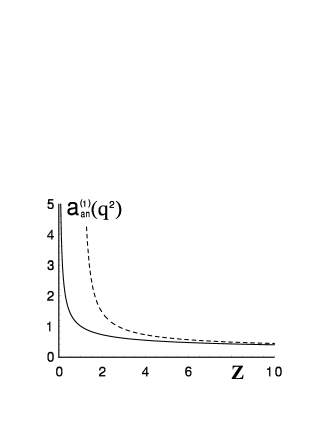
Figure 1: The one-loop perturbative coupling (dashed curve) and the analytic charge (Eq. (4)) (solid curve), $a(q^{2})=\alpha(q^{2})\beta_{0}/(4\pi),\;z=q^{2}/\Lambda^{2}$.

In this talk we will outline how the behavior of the running coupling (5) is affected by the pion mass entering the Adler $D$ function, thus giving rise to an infrared finite value for this coupling. We will also argue that this analytic effective charge may be relevant to the study of chiral symmetry breaking (CSB) through the Schwinger-Dyson equations.

A certain insight into the nonperturbative aspects of the strong interaction can be provided by the Adler $D$ function [4]

$$D(q^{2})=\frac{d\,\Pi(q^{2})}{d\ln q^{2}},$$ (7)

with $\Pi(q^{2})$ being hadronic vacuum polarization function. In particular, Eq. (7) is related to the measurable ratio $R(s)$ of the $e^{+}e^{-}$ annihilation into hadrons through the dispersion relation [4]

$$D(q^{2})=q^{2}\int_{4m_{\pi}^{2}}^{\infty}\frac{R(s)}{(s+q^{2})^{2}}\,ds.$$ (8)

In turn, this equation implies the definite analytic properties in the $q^{2}$ variable for $D(q^{2})$: it is an analytic function in the complex $q^{2}$-plane with the only cut beginning at the two–pion threshold $-\infty<q^{2}\leq-4m_{\pi}^{2}$ along the negative semiaxis of real $q^{2}$.

In the ultraviolet domain the Adler $D$ function is usually computed in the framework of perturbation theory:

$$D(q^{2})=3\sum_{f}Q_{f}^{2}\left[1+d(q^{2})\right],$$ (9)

where $Q_{f}$ is the charge of the $f$-th quark,

$$d(q^{2})\simeq d_{1}\left[\frac{\alpha_{\mbox{\scriptsize s}}(q^{2})}{\pi}\right]+d_{2}\left[\frac{\alpha_{\mbox{\scriptsize s}}(q^{2})}{\pi}\right]^{2}+\ldots,$$ (10)

$d_{1}=1$, $d_{2}\simeq 1.9857-0.1153\,n_{\mbox{\scriptsize f}}$, and $n_{\mbox{\scriptsize f}}$ is the number of active quarks. However, such approximation of Eq. (10) violates the analyticity condition that $D(q^{2})$ must satisfy, due to the spurious singularities of the perturbative running coupling $\alpha_{\mbox{\scriptsize s}}(q^{2})$. Nevertheless, this difficulty, which is an artifact of the perturbative treatment, can be eliminated by imposing the analyticity requirement of the form

$$d(q^{2},m_{\pi}^{2})=\int_{4m_{\pi}^{2}}^{\infty}\frac{\varkappa(\sigma)}{\sigma+q^{2}}\,d\sigma$$ (11)

on the right hand-side of Eq. (10). Therefore, the QCD effective charge itself has to satisfy the integral representation

$$\alpha^{(\ell)}_{\mbox{\scriptsize an}}(q^{2},m_{\pi}^{2})=\frac{4\pi}{\beta_{0}}\!\int_{\chi}^{\infty}\!\frac{\rho^{(\ell)}(\sigma)}{\sigma+z}\,d\sigma,\;\;\chi=\frac{4m_{\pi}^{2}}{\Lambda^{2}},$$ (12)

where $\rho^{(\ell)}(\sigma)$ is the $\ell$-loop spectral density [3, 5].

The behavior of the one-loop massive analytic charge (12) in the spacelike and timelike infrared domains is shown in Figure 2. The value of $\Lambda=(623\pm 81)\,$MeV is found by making use of the experimental data on the inclusive $\tau$ lepton decay [6]. It is worth noting that the nonvanishing pion mass drastically affects the infrared behavior of the analytic coupling in hand: instead of the enhancement in the massless case (5) one has here a finite infrared limiting value of the effective charge (12) (see also Refs. [5, 6] for the details).

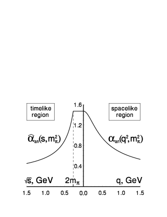
Figure 2: The one–loop massive analytic effective charge (12) in the spacelike and timelike domains. The values of parameters are: $n_{\mbox{\scriptsize f}}=2$ active quarks, $\Lambda=623\,$MeV.

Based on the study of the gauge invariant Schwinger-Dyson equations, Cornwall proposed a long time ago that the self-interactions of gluons give rise to a dynamical gluon mass, while preserving at the same time the local gauge symmetry of the theory [7]. This gluon “mass” is not a directly measurable quantity, but must be related to other physical parameters, such as the glueball spectrum, the energy needed to pop two gluons out of the vacuum, the QCD string tension, or the QCD vacuum energy.

One of the main phenomenological implications of this analysis is that the presence of the gluon mass $m_{g}$ saturates the running of the strong coupling, forcing it to “freeze” in the infrared domain. In particular, the nonperturbative effective coupling obtained in Ref. [7] is given by

$$\alpha_{\mbox{\tiny C}}(q^{2})=\frac{4\pi}{\beta_{0}}\frac{1}{\ln\!\left[z+4M_{g}^{2}(q^{2})/\Lambda^{2}\right]},$$ (13)

where $M_{g}(q^{2})$ is the dynamical gluon mass

$$M^{2}_{g}(q^{2})=m_{g}^{2}\left[\frac{\ln\left(z+4m_{g}^{2}/\Lambda^{2}\right)}{\ln\left(4m_{g}^{2}/\Lambda^{2}\right)}\right]^{-12/11}.$$ (14)

The coupling (13) has the infrared finite limiting value $\alpha_{\mbox{\tiny C}}(0)=4\pi\left[\beta_{0}\ln(4m_{g}^{2}/\Lambda^{2})\right]^{-1}$. For a typical values of $m_{g}=500\,$MeV and $\Lambda=300\,$MeV, one obtains for the case of pure gluodynamics ($n_{\mbox{\scriptsize f}}=0$) an estimation $\alpha_{\mbox{\tiny C}}(0)\simeq 0.5$. An independent analysis [8] yields a maximum allowed value for $\alpha_{\mbox{\tiny C}}(0)$ of about 0.6. The incorporation of fermions into the effective charge [9]

$$\alpha_{\mbox{\scriptsize cp}}(q^{2})=\frac{4\pi}{11\ln(z+\chi_{g})-2n_{\mbox{\scriptsize f}}\ln(z+\chi_{q})/3}$$ (15)

does not change the picture qualitatively (at least for quark masses of the order of $\Lambda$). In equation (15) $\chi_{g}=4m_{g}^{2}/\Lambda^{2}$, $\chi_{q}=4m_{q}^{2}/\Lambda^{2}$, $m_{g}=(500\pm 100)\,$MeV stands for the gluon mass and $m_{q}=350\,$MeV is a light quark constituent mass.

The effective coupling of Eq. (13) was the focal point of extensive scrutiny, and has been demonstrated to furnish a unified description of a wide variety of the low energy QCD data [10].

However, an important unresolved question in this context is the incorporation of the QCD effective charge into the standard Schwinger-Dyson equation governing the dynamics of the quark propagator $S(p)$

$$S^{-1}(p)=S_{0}^{-1}(p)-g^{2}\int\frac{d^{4}k}{(2\pi)^{4}}\gamma_{\mu}\,S\,\Gamma_{\nu}\,\Delta^{\mu\nu}.$$ (16)

Specifically, since QCD is not a fixed point theory, the usual QED-inspired gap equation must be modified, in order to incorporate the running charge and asymptotic freedom. The usual way of accomplishing this eventually boils down to the replacement $1/k^{2}\to\alpha(k^{2})/k^{2}$ in the corresponding kernel of the gap equation, where $\alpha(k^{2})$ is the QCD running coupling. The inclusion of $\alpha(k^{2})$ is essential for arriving at an integral equation for $S(p)$ which is well-behaved in the ultraviolet. However, since the perturbative form of $\alpha(k^{2})$ diverges at low energies as $1/\ln(k^{2}/\Lambda^{2})$ when $k^{2}\to\Lambda^{2}$, some form of the infrared regularization for $\alpha(k^{2})$ is needed, whose details depend on the specific assumptions one is making regarding the nonperturbative hadron dynamics. At this point the issue of the critical coupling makes its appearance. Specifically, as is well-known, there is a critical infrared limiting value of the running coupling, to be denoted by $\alpha_{\mbox{\scriptsize cr}}$, below which there are no nontrivial solutions to the resulting gap equation, i.e., there is no CSB, see Fig. 3.

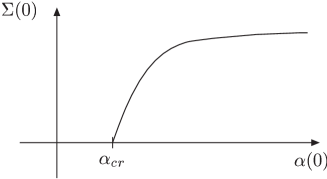
Figure 3: A typical dependence of $\Sigma(0)$ on the limiting value $\alpha(0)$, $\,S^{-1}(p)=A(p)p/+\Sigma(p)$.

The incorporation of the effective charge of Eq. (13) into a gap equation has been studied for the first time in Ref. [11]. There it was concluded that CSB solutions for $\Sigma(p)$ could be obtained only for unnaturally small values of the gluon mass, namely $m_{g}/\Lambda\simeq 0.8$. This is so because the typical value of $\alpha_{\mbox{\scriptsize cr}}$ found in the standard treatment of the gap equation is $\alpha_{\mbox{\scriptsize cr}}\simeq 1.2$, which is what the expression for $\alpha_{\mbox{\tiny C}}(0)$ yields for the above value of $m_{g}/\Lambda$. This issue was further investigated in Ref. [9], where a system of coupled gap and vertex equations was considered. The upshot of this study was that no consistent solutions to the system of integral equations could be found, due to the fact that the allowed values for $\alpha(0)$, dictated by the vertex equation, were significantly lower than $\alpha_{\mbox{\tiny C}}(0)$, i.e., not large enough to trigger chiral symmetry breaking.

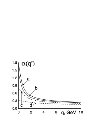
Figure 4: Comparison of the massive analytic running coupling (Eq. (12), solid curves) with the effective charge (15) (dashed curves). The values of parameters are: $n_{\mbox{\scriptsize f}}=2$ active quarks, $\Lambda=704\,$MeV (a), $\Lambda=542\,$MeV (b), gluon mass $m_{g}=400\,$MeV and $\Lambda=350\,$MeV (c), gluon mass $m_{g}=600\,$MeV and $\Lambda=150\,$MeV (d).

In what follows we will suggest a possible resolution of this problem. The basic observation is captured in Figure 4: the effective charge with a gluon mass (dashed curves) and the analytic charge (12) (solid curves) coincide for a large range of momenta, and they only begin to differ appreciably in the deep infrared domain ($k^{2}\lesssim\Lambda^{2}$). In this region the analytic charge (12) rises abruptly, almost doubling its size between $k^{2}=\Lambda^{2}$ and $k^{2}=0$, whereas the running coupling (15) in the same momentum interval remains essentially fixed to a value of about 0.6. A possible picture that seems to emerge from this observation is the following. It may be that the concept of the dynamically generated gluon mass fails to capture all the relevant dynamics in the very deep infrared, where confinement or other nonperturbative effects make their appearance. At that point it may be preferable to switch to a description in terms of the analytic charge (12), which (i) coincides with that of Cornwall in the region where the latter furnishes a successful description of data, and (ii) in addition, because it overcomes the critical value $\alpha_{\mbox{\scriptsize cr}}$, offers the possibility of accounting for CSB at the level of gap equations. It would be interesting to carry out a detailed study of the gap equation, with the analytic charged plugged into, in order to verify if indeed one encounters nontrivial solutions, whose size is phenomenologically relevant, and if a reasonable value of the pion-decay constant $f_{\pi}$ may be obtained.

References

- [1] P.J. Redmond, Phys. Rev. 112, 1404 (1958); N.N. Bogoliubov, A.A. Logunov, and D.V. Shirkov, Sov. Phys. JETP 37, 574 (1960).
- [2] D.V. Shirkov and I.L. Solovtsov, Phys. Rev. Lett. 79, 1209 (1997).
- [3] A.V. Nesterenko, Phys. Rev. D 62, 094028 (2000); Phys. Rev. D 64, 116009 (2001); Int. J. Mod. Phys. A 18, 5475 (2003).
- [4] S.L. Adler, Phys. Rev. D 10, 3714 (1974).
-
[5]
A.V. Nesterenko and J. Papavassiliou,
arXiv:hep-ph/0409220. - [6] A.V. Nesterenko and J. Papavassiliou, in preparation.
- [7] J.M. Cornwall, Phys. Rev. D 26, 1453 (1982).
- [8] J.M. Cornwall and J. Papavassiliou, Phys. Rev. D 40, 3474 (1989).
- [9] J. Papavassiliou and J.M. Cornwall, Phys. Rev. D 44, 1285 (1991).
- [10] A.C. Aguilar, A. Mihara and A.A. Natale, Int. J. Mod. Phys. A 19, 249 (2004).
- [11] B. Haeri and M.B. Haeri, Phys. Rev. D 43, 3732 (1991).