Abstract

The decays $\tilde{\nu}_{e}\to e^{-}\tilde{\chi}_{1}^{+}$, $\tilde{\nu}_{e}^{*}\to e^{+}\tilde{\chi}_{1}^{-}$, when kinematically allowed, constitute a source of 100% polarised charginos. We study the process $e^{+}e^{-}\to\tilde{\nu}_{e}^{*}\tilde{\nu}_{e}\to e^{+}\tilde{\chi}_{1}^{-}\,e^{-}\tilde{\chi}_{1}^{+}$, with subsequent chargino decays $\tilde{\chi}_{1}^{-}\to\bar{\nu}_{\mu}\mu^{-}\tilde{\chi}_{1}^{0}$, $\tilde{\chi}_{1}^{+}\to q\bar{q}^{\prime}\tilde{\chi}_{1}^{0}$ or their charge conjugate $\tilde{\chi}_{1}^{-}\to\bar{q}q^{\prime}\tilde{\chi}_{1}^{0}$, $\tilde{\chi}_{1}^{+}\to\nu_{\mu}\mu^{+}\tilde{\chi}_{1}^{0}$. The kinematics of this process allows the reconstruction of the sneutrino and chargino rest frames, and thus a clean analysis of the angular distributions of the visible final state products in these reference systems. Furthermore, a triple product CP asymmetry can be built in $\tilde{\chi}_{1}^{\pm}$ hadronic decays, involving the chargino spins and the momenta of the quark and antiquark. With a good $c$ tagging efficiency, this CP asymmetry is quite sensitive to the phase of the bino mass term $M_{1}$ and can test CP violation in the neutralino sector.

1 Introduction

An international linear $e^{+}e^{-}$ collider (ILC) offers an ideal environment for the study of supersymmetry (SUSY) [1, 2], if this theory is realised in nature. With adequate choices for the centre of mass (CM) energy and beam polarisations, the various production processes simultaneously present in $e^{+}e^{-}$ annihilation can be disentangled. It is then possible to measure sparticle masses, couplings and mixings [3], allowing for the determination of the Lagrangian parameters. The quantum numbers of the new particles must be investigated as well, in order to confirm that they are the superpartners of the Standard Model (SM) fields. In particular, it is crucial to determine the spins of the SUSY particles. Spin-dependent effects serve not only to deduce the particle spins but may also be used to verify the predictions of the theory, using the input from other experiments. It is also conceivable that spin distributions and asymmetries, if precisely measured, can be used to improve the measurement of some of the mixing parameters of the Lagrangian.

The existence of purely supersymmetric CP violation sources is other of the aspects that require a thorough investigation. At present, all CP violation observed in $K$ and $B$ oscillations and decay (with the possible exception of the time-dependent CP asymmetry in $B_{d}^{0}\to\phi K_{S}$, whose experimental situation is still unclear) can be explained by a single CP-violating phase in the Cabibbo-Kobayashi-Maskawa mixing matrix. However, the CP breaking induced by this phase cannot account for the observed baryon asymmetry in the universe. The most general Lagrangian of the minimal supersymmetric Standard Model (MSSM) contains a large number of CP violation sources, which can potentially yield observable effects at low and high energies. Within the neutralino sector, CP-violating phases can appear in the bino and Higgsino mass terms, $M_{1}$ and $\mu$, respectively. At low energies the phases $\phi_{1}$, $\phi_{\mu}$ of these two parameters generally lead to unacceptably large SUSY contributions to electric dipole moments (EDMs), if they are different from $0,\pi$. Present constraints from EDMs place strong restrictions on the values of $\phi_{1}$ and $\phi_{\mu}$, but do not necessarily require that $M_{1}$ and $\mu$ are real, and cancellations among the different SUSY contributions can occur [4, 5, 6]. This possibility, and the need for further CP violation sources beyond the SM, makes the investigation of CP breaking in the neutralino sector a compelling task to be carried out at a linear collider.

In this paper we focus on the determination of the spin and spin-related properties of sneutrinos and charginos, including CP-violating spin asymmetries in chargino decays. We study sneutrino pair production in $e^{+}e^{-}$ annihilation at a CM energy of 800 GeV, as proposed for an ILC upgrade. We concentrate in the channels

$$e^{+}e^{-} \to\tilde{\nu}_{e}^{*}\tilde{\nu}_{e}\to e^{+}\tilde{\chi}_{1}^{-}\,e^{-}\tilde{\chi}_{1}^{+}\to e^{+}\bar{\nu}_{\mu}\mu^{-}\tilde{\chi}_{1}^{0}\,e^{-}q\bar{q}^{\prime}\tilde{\chi}_{1}^{0}\,,$$

$$e^{+}e^{-} \to\tilde{\nu}_{e}^{*}\tilde{\nu}_{e}\to e^{+}\tilde{\chi}_{1}^{-}\,e^{-}\tilde{\chi}_{1}^{+}\to e^{+}\bar{q}q^{\prime}\tilde{\chi}_{1}^{0}\,e^{-}\nu_{\mu}\mu^{+}\tilde{\chi}_{1}^{0}\,,$$ (1)

with $q=u,c$, $q^{\prime}=d,s$. This process has three advantages for our purposes: (i) the charginos produced are 100% polarised, having positive helicity in the decay $\tilde{\nu}_{e}^{*}\to e^{+}\tilde{\chi}_{1}^{-}$ and negative helicity in $\tilde{\nu}_{e}\to e^{-}\tilde{\chi}_{1}^{+}$; (ii) the kinematics allows the determination of the sneutrino and chargino rest frames, and then the study of angular distributions in these reference systems; (iii) its cross section is large, and backgrounds with 5 energetic final state particles plus large missing energy and momentum are small. Muon sneutrinos are also a source of polarised charginos, but the cross section for $\tilde{\nu}_{\mu}^{*}\tilde{\nu}_{\mu}$ production is much smaller. Beam polarisations $P_{e^{-}}=-0.8$, $P_{e^{+}}=0.6$ can be used to increase the signal cross sections but they do not affect the angular distributions and CP asymmetries studied.

For definiteness, we consider a SUSY scenario like SPS1a in Ref. [7] but with a heavier slepton spectrum (and nonzero phases $\phi_{1}$, $\phi_{\mu}$), so that sneutrino decays to charginos are kinematically allowed. The analysis of $e^{-}$, $e^{+}$ angular distributions in the $\tilde{\nu}_{e}$, $\tilde{\nu}_{e}^{*}$ rest frames provides a strong indication that sneutrinos are scalar particles and charginos have spin $1/2$. The angular distributions of the $\tilde{\chi}_{1}^{-}$ ($\tilde{\chi}_{1}^{+}$) decay products $\mu^{-}$, $\bar{q}$, $q^{\prime}$ ($\mu^{+}$, $q$, $\bar{q}^{\prime}$) with respect to the $\tilde{\chi}_{1}^{-}$ ($\tilde{\chi}_{1}^{+}$) spin can be precisely measured as well. Furthermore, summing $\tilde{\chi}_{1}^{-}$ and $\tilde{\chi}_{1}^{+}$ hadronic decays, a CP asymmetry based on the triple product $\vec{s}_{\pm}\cdot(\vec{p}_{\bar{q}_{1}}\times\vec{p}_{q_{2}})$ can be built, where $\vec{s}_{\pm}$ is the spin direction of the $\tilde{\chi}_{1}^{-}$ or $\tilde{\chi}_{1}^{+}$, and $\vec{p}_{\bar{q}_{1}}$, $\vec{p}_{q_{2}}$ are the three-momenta of the antiquark and quark resulting from its decay, respectively, in the $\tilde{\chi}_{1}^{\pm}$ rest frame. A good $c$ tagging efficiency, as expected for a future linear collider, is essential for the determination of quark angular distributions and the CP asymmetry. For the latter it is necessary to distinguish between the quark and antiquark produced in the decay. This can be done combining $c$ tagging and the knowledge of the final state muon charge.

We note that in chargino pair production $e^{+}e^{-}\to\tilde{\chi}_{1}^{+}\tilde{\chi}_{1}^{-}$ the charginos are polarised as well [8], allowing for the measurement of decay angular distributions and CP-violating asymmetries. However, in this process the momenta of the decaying charginos cannot be determined with kinematical constraints, and thus the analysis of angular distributions is less clean. Moreover, the backgrounds for $\tilde{\chi}_{1}^{+}\tilde{\chi}_{1}^{-}$ in the semileptonic decay channel are huge, being $e^{+}e^{-}\to W^{+}W^{-}\to\ell^{\pm}\nu jj$, $\ell=e,\mu$ the most troublesome, with a cross section (including ISR and beamstrahlung corrections) of approximately 3.5 pb at CM energies of 500 and 800 GeV, for $P_{e^{+}}=0.6$, $P_{e^{-}}=-0.8$. At any rate, in SUSY scenarios where sneutrino decays to charginos are not kinematically allowed, $\tilde{\chi}_{1}^{+}\tilde{\chi}_{1}^{-}$ production seems the best place for the study of chargino spin properties and CP asymmetries in chargino decays.

This paper is organised as follows. In section 2 we discuss sneutrino production and decay, focusing on the features most relevant for our work, and fix the SUSY scenario used. The procedure for the Monte Carlo calculation of the processes and reconstruction of the signals is outlined in section 3. In section 4 we introduce the different distributions analysed and present our numerical results. In section 5 we compare with results obtained from other processes and draw our conclusions.

2 Production and decay of sneutrino pairs

Sneutrino pairs are produced in $e^{+}e^{-}$ collisions through the Feynman diagrams depicted in Fig. 1. Their two-body decays $\tilde{\nu}_{e}\to e^{-}\tilde{\chi}_{1}^{+}$, $\tilde{\nu}_{e}^{*}\to e^{+}\tilde{\chi}_{1}^{-}$ are mediated by the $\tilde{\nu}_{e}e\tilde{\chi}_{1}^{-}$ vertex which, neglecting the electron Yukawa coupling, is given by

$$\mathcal{L}_{\tilde{\nu}_{e}e\tilde{\chi}_{1}^{-}} = -gV_{11}\,\bar{e}\,P_{R}\,\tilde{\chi}_{1}^{-}\;\tilde{\nu}_{e}-gV_{11}^{*}\,\overline{\tilde{\chi}_{1}^{-}}\,P_{L}\,e\;\tilde{\nu}_{e}^{*}\,,$$ (2)

with $V^{\dagger}$ the $2\times 2$ unitary matrix diagonalising the chargino mass matrix by the right (the interactions and notation used can be found in Refs. [9, 10], and follow the conventions of Ref. [11]). By inspection of the Lagrangian it is easily seen that in the decay $\tilde{\nu}_{e}\to e^{-}\tilde{\chi}_{1}^{+}$, mediated by the first term in Eq. (2), the produced electron has negative chirality (and thus negative helicity, neglecting the electron mass) and the chargino has positive chirality. Since sneutrinos are spinless particles, angular momentum conservation in the $\tilde{\nu}_{e}$ rest frame implies that the $\tilde{\chi}_{1}^{+}$ must have negative helicity as well, as depicted schematically in Fig. 2 (a). For $\tilde{\nu}_{e}^{*}\to e^{+}\tilde{\chi}_{1}^{-}$, the positron has negative chirality, and thus positive helicity; therefore, the $\tilde{\chi}_{1}^{-}$ has positive helicity in the $\tilde{\nu}_{e}^{*}$ rest frame, as shown in Fig. 2 (b).

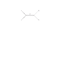
Figure 1: Feynman diagrams for $\tilde{\nu}_{e}^{*}\tilde{\nu}_{e}$ production in $e^{+}e^{-}$ annihilation.

(a)		(b)

Figure 2: Helicity of the charginos produced in $\tilde{\nu}_{e}$ and $\tilde{\nu}_{e}^{*}$ decays.

The decay of $\tilde{\chi}_{1}^{-}$ to light fermions $\bar{f},f^{\prime}$ and a neutralino $\tilde{\chi}_{1}^{0}$ is mediated by the diagrams in Fig. 3, with similar diagrams for $\tilde{\chi}_{1}^{+}$ decay. We study final states in which one of the charginos decays leptonically and the other hadronically. In leptonic decays we restrict ourselves to $\bar{f}f^{\prime}=\bar{\nu}_{\mu}\mu^{-}$ ($f\bar{f}^{\prime}=\nu_{\mu}\mu^{+}$). The reason is that in decays to $e^{\pm}$ and a neutrino, the presence of an additional $e^{+}e^{-}$ pair from sneutrino decays difficults the reconstruction of the final state, while in decays to $\tau^{\pm}$ the momentum of the charged lepton cannot be directly measured. We sum all hadronic decays $\bar{f}f^{\prime}=\bar{u}d,\bar{c}s$ ($f\bar{f}^{\prime}=u\bar{d},c\bar{s}$).

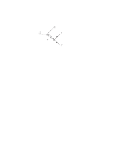
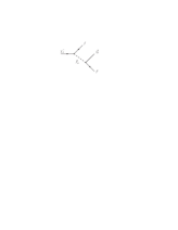
(a)		(b)		(c)

Figure 3: Feynman diagrams for the decay $\tilde{\chi}_{1}^{-}\to\bar{f}f^{\prime}\tilde{\chi}_{1}^{0}$, for light fermions $\bar{f}f^{\prime}=\bar{\nu}_{e}e^{-},\bar{\nu}_{\mu}\mu^{-},\bar{u}d,\bar{c}s$ and negligible $\tilde{f}^{\prime}_{L}-\tilde{f}^{\prime}_{R}$, $\tilde{f}_{L}-\tilde{f}_{R}$ mixing. For $f=\nu_{\ell}$, in diagram (c) $\tilde{f}_{L}^{*}=\tilde{\nu}_{\ell}^{*}$ is exchanged.

We choose a SUSY scenario similar to SPS1a but with a heavier sfermion spectrum and complex phases $\phi_{1}$, $\phi_{\mu}$. The low-energy parameters most important for our analysis are collected in Table 1. For vanishing $\phi_{1}$, $\phi_{\mu}$, they approximately correspond to $m_{1/2}=250$ GeV, $m_{\tilde{E}}=m_{\tilde{L}}=m_{H_{i}}=200$ GeV, $A_{E}=-200$ GeV at the unification scale, and $\tan\beta=10$. We use SPheno [12] to calculate sparticle masses, mixings and some decay widths. Neutralino and chargino masses slightly depend on $\phi_{1}$, $\phi_{\mu}$; for $\phi_{1}=\phi_{\mu}=0$ they are $m_{\tilde{\chi}_{1}^{0}}=99$ GeV, $m_{\tilde{\chi}_{1}^{-}}=178$ GeV, $m_{\tilde{\chi}_{2}^{-}}=401$ GeV. The relevant branching ratios (taking $\phi_{1}=\phi_{\mu}=0$) are $\mathrm{Br}(\tilde{\nu}_{e}\to e^{-}\,\tilde{\chi}_{1}^{+})=0.52$, $\mathrm{Br}(\tilde{\chi}_{1}^{-}\to\bar{\nu}_{\mu}\mu^{-}\tilde{\chi}_{1}^{0})=0.10$, $\mathrm{Br}(\tilde{\chi}_{1}^{-}\to\bar{q}q^{\prime}\tilde{\chi}_{1}^{0})=0.34$, with the same rates for the charge-conjugate processes.

Parameter		Value
$M_{1}$		102.0 $e^{i\phi_{1}}$
$M_{2}$		192.0
$\mu$		377.5 $e^{i\phi_{\mu}}$
$\tan\beta$		10
$m_{\tilde{\nu}_{e}}$		252.4
$m_{\tilde{\mu}_{L}}$		264.5
$m_{\tilde{u}_{L}},m_{\tilde{c}_{L}}$		571.5
$m_{\tilde{d}_{L}},m_{\tilde{s}_{L}}$		577.0

Table 1: Low-energy parameters (at the scale $M_{Z}$) for the SUSY scenario used. The dimensionful parameters are in GeV.

In the scenario selected the three-body decays $\tilde{\chi}_{1}^{-}\to f\bar{f}^{\prime}\tilde{\chi}_{1}^{0}$ are mediated by off-shell intermediate particles. Still, they are dominated by $W$ exchange, diagram (a) in Fig. 3, due to the large sfermion masses. In $\tilde{\chi}_{1}^{-}\to\bar{\nu}_{\mu}\mu^{-}\tilde{\chi}_{1}^{0}$ the second diagram in importance is sneutrino exchange in diagram 3 (c), but its contribution to the partial width is 13 times smaller than the one from $W$ exchange. For hadronic decays, diagrams involving squarks are even more suppressed, and their contribution has a relative magnitude of $2\times 10^{-4}$ with respect to the $W$ diagram. Therefore, many characteristics of this scenario are shared with scenarios with a heavier chargino spectrum, in which the two-body decay $\tilde{\chi}_{1}^{-}\to W^{-}\tilde{\chi}_{1}^{0}$ is possible and diagrams (b) and (c) are negligible both for leptonic and hadronic final states.

For values of $\phi_{1}$, $\phi_{\mu}$ different from $0,\pi$, CP is violated in the neutralino and chargino sectors, leading to large SUSY contributions to EDMs. If the squark spectrum (which does not play any role in our analysis, as seen from the previous discussion) is heavy enough, experimental limits on the neutron and Mercury EDMs can be satisfied. On the other hand, for the selectron and sneutrino masses under consideration, the experimental bound on the electron EDM $d_{e}$ severely constrains the allowed region in the $(\phi_{1},\phi_{\mu})$ plane. Using the expressions for $d_{e}$ in Ref. [13] it is found that, for each $\phi_{1}$ between 0 and $2\pi$, in this scenario there exist two narrow intervals for $\phi_{\mu}$, one with values $\phi_{\mu}\sim 0$ and the other with values $\phi_{\mu}\sim\pi$, in which the neutralino and chargino contributions to $d_{e}$ partially cancel, resulting in a value compatible with the experimental limit $d_{e}^{\mathrm{\,exp}}=(0.079\pm 0.074)\times 10^{-26}~{}e$ cm [14]. For instance, for $\phi_{1}=\pi/2$ the phase $\phi_{\mu}$ can be $\phi_{\mu}\simeq-0.12$ or $\phi_{\mu}\simeq 3.21$. Several representative examples of these pairs of phases allowed by EDM constraints are collected in Table 2. We can see that in principle it is possible to have any phase $\phi_{1}$, though with a strong correlation with $\phi_{\mu}$. If $\phi_{1}$ and $\phi_{\mu}$ are experimentally found to be non-vanishing, a satisfactory explanation will be necessary for this correlation, which apparently would be a “fine tuning” of their values [15].

$\phi_{1}$	$\phi_{\mu}$		$\phi_{1}$	$\phi_{\mu}$
0	0		$\pi$	0
$\pi/8$	-0.0476		$7\pi/8$	-0.0454
$\pi/4$	-0.0876		$3\pi/4$	-0.0845
$3\pi/8$	-0.1136		$5\pi/8$	-0.1114
$\pi/2$	-0.1218

Table 2: Examples of approximate phases $\phi_{1}$, $\phi_{\mu}$ for which the pairs $(\phi_{1},\phi_{\mu})$, $(-\phi_{1},-\phi_{\mu})$ are allowed by EDM constraints.

3 Generation and reconstruction of the signals

The matrix element of the resonant processes in Eq. (1) are calculated using HELAS [16], including all spin correlations and finite width effects. The relevant terms of the Lagrangian can be found in Refs. [9, 10]. We assume a CM energy of 800 GeV, with electron polarisation $P_{e^{-}}=-0.8$ and positron polarisation $P_{e^{+}}=0.6$. Beam polarisation has no effect on the angular distributions and asymmetries studied but increases the signal cross section. The luminosity is taken as 534 fb^-1 per year [17]. In our calculations we take into account the effects of initial state radiation (ISR) [18] and beamstrahlung [19, 20]. For the design luminosity at 800 GeV we use the parameters $\Upsilon=0.09$, $N=1.51$ [17]. The actual expressions for ISR and beamstrahlung used in our calculation are collected in Ref. [9]. We also include a beam energy spread of 1%.

We simulate the calorimeter and tracking resolution of the detector by performing a Gaussian smearing of the energies of electrons ($e$), muons ($\mu$) and jets ($j$), using the specifications in Ref. [21],

$$\frac{\Delta E^{e}}{E^{e}}=\frac{10\%}{\sqrt{E^{e}}}\oplus 1\%\;,\quad\frac{\Delta E^{\mu}}{E^{\mu}}=0.02\%\,E^{\mu}\;,\quad\frac{\Delta E^{j}}{E^{j}}=\frac{50\%}{\sqrt{E^{j}}}\oplus 4\%\;,$$ (3)

where the two terms are added in quadrature and the energies are in GeV. We apply kinematical cuts on transverse momenta, $p_{T}\geq 10$ GeV, and pseudorapidities $|\eta|\leq 2.5$, the latter corresponding to polar angles $10^{\circ}\leq\theta\leq 170^{\circ}$. We also reject events in which the leptons or jets are not isolated, requiring a “lego-plot” separation $\Delta R=\sqrt{\Delta\eta^{2}+\Delta\phi^{2}}\geq 0.4$. For the Monte Carlo integration in 10-body phase space we use RAMBO [22].

For the precise measurement of angular distributions it is crucial to reconstruct accurately the final state. This is more difficult when several particles escape detection, as it happens in our case. Since we are not interested in the mass distributions we use as input all the sparticle masses involved, which we assume measured in other processes [3]. Let us label the electron and positron 4-momenta as $p_{e^{-}}$, $p_{e^{+}}$, respectively, and the momenta of the “visible” chargino decay products (the $\mu^{\pm}$ for the leptonic decay and the quark-antiquark pair in the hadronic decay) as $p_{V^{+}}$, $p_{V^{-}}$. The unknown momenta of the “invisible” chargino decay products (the $\nu\tilde{\chi}_{1}^{0}$ pair in leptonic decays and the neutralino in hadronic decays) are $p_{I^{+}}$, $p_{I^{-}}$ (8 unknowns). From four-momentum conservation and the kinematics of the process we have the relations

$$E_{I^{+}}+E_{I^{-}} =E_{\mathrm{CM}}-E_{e^{-}}-E_{e^{+}}-E_{V^{+}}-E_{V^{-}}\,,$$

$$\vec{p}_{I^{-}}+\vec{p}_{I^{+}} =\vec{p}\!\!\!\!\!\not\,\,\,\,\,,$$

$$(p_{V^{+}}+p_{I^{+}})^{2} =m_{\tilde{\chi}_{1}^{-}}^{2}\,,$$

$$(p_{V^{-}}+p_{I^{-}})^{2} =m_{\tilde{\chi}_{1}^{-}}^{2}\,,$$

$$(p_{e^{-}}+p_{V^{+}}+p_{I^{+}})^{2} =m_{\tilde{\nu}_{e}}^{2}\,,$$

$$(p_{e^{+}}+p_{V^{-}}+p_{I^{-}})^{2} =m_{\tilde{\nu}_{e}}^{2}\,,$$ (4)

where $E_{\mathrm{CM}}$ is the CM energy and $\vec{p}\!\!\!\!\!\not\,\,\,\,$ the missing momentum. These 8 equations are at most quadratic in the unknown momenta $p_{I^{+}}$, $p_{I^{-}}$. With a little algebra, they can be written in the form of 7 linear plus one quadratic equation, which can be solved yielding 2 possible solutions for the unknown momenta (note that in leptonic decays only the sum of the neutrino and neutralino momenta can be determined). In order to select the correct one we use the additional constraint that either $p_{I^{+}}^{2}=m_{\tilde{\chi}_{1}^{0}}^{2}$ or $p_{I^{-}}^{2}=m_{\tilde{\chi}_{1}^{0}}^{2}$ depending on which chargino decays hadronically (this is decided event by event depending on the charge of the muon). With $p_{I^{+}}$, $p_{I^{-}}$ obtained from the reconstruction process, the momenta of the two charginos and the two sneutrinos can be determined, as well as their respective rest frames.

We note that ISR, beamstrahlung, particle width effects and detector resolution degrade the determination of $p_{I^{+}}$, $p_{I^{-}}$, being ISR and beamstrahlung the most troublesome. Detector resolution affects the measurement of charged lepton and jet momenta, while ISR and beamstrahlung modify the beam energies and thus reduce the CM energy, causing also that the CM and laboratory frames do not coincide. Moreover, the last four of Eqs. (4) only hold for strictly on-shell sneutrinos and charginos. Due to these effects, Eqs. (4) sometimes do not have a real solution, i.e. the discriminant of the quadratic equation mentioned above is negative. In such case, we force the system to have a real solution by setting the discriminant to zero, what has the consequence that the solutions do not fulfill Eqs. (4) for the input values $m_{\tilde{\chi}_{1}^{-}}$, $m_{\tilde{\nu}_{e}}$ used but rather for other (sometimes very different) ones.

The determination of the unknown momenta is done as follows. In order to partially take into account the decrease in the CM energy we replace $E_{\mathrm{CM}}$ in Eq. (4) by an “effective” CM energy $E_{\mathrm{CM}}^{\mathrm{eff}}$. We try the reconstruction of the unknown momenta for different energies $E_{\mathrm{CM}}^{\mathrm{eff}}\leq E_{\mathrm{CM}}$ in decreasing order, choosing the one which gives reconstructed sneutrino, chargino and neutralino masses closest to their true values. In case that different effective energies yield equal results for the reconstructed masses, we choose the largest one. If the event does not reasonably fit into the kinematics assumed for the process, it is discarded.

For the analysis of some observables we take advantage of the good $c$ tagging capability that it is expected at a future linear collider. We use a $c$ tagging efficiency of 50% and a mistag rate of 0.2% [23]. The identification of $c$ against $\bar{c}$, when needed, can be indirectly done looking at the charge of the muon produced. In final states with $\mu^{-}$, the chargino decaying hadronically is $\tilde{\chi}_{1}^{+}$, thus the tagged jet corresponds to a $c$ quark and the other one to a $s$ antiquark. By the same argument, for $\mu^{+}$ final states the tagged jet corresponds to a $c$ antiquark and the other one to a $s$ quark.

The backgrounds to the processes in Eq. (1) are rather small. Other SUSY particle production processes leading to a final state of $e^{+}e^{-}\mu^{\pm}jj$ plus large missing energy and momentum are for instance $e^{+}e^{-}\to\tilde{\chi}_{1}^{\pm}\tilde{\chi}_{2}^{\mp}\to\tilde{\chi}_{1}^{\pm}\;Z\tilde{\chi}_{1}^{\mp}$, $e^{+}e^{-}\to\tilde{\chi}_{1}^{\pm}\tilde{\chi}_{2}^{\mp}\to\tilde{\chi}_{1}^{\pm}\;W^{\mp}\tilde{\chi}_{2}^{0}$, $e^{+}e^{-}\to\tilde{\chi}_{2}^{0}\tilde{\chi}_{3,4}^{0}\to\tilde{\chi}_{2}^{0}\,\tilde{\chi}_{1}^{\pm}\tilde{W}^{\mp}$, with subsequent decays $Z\to e^{+}e^{-}$, $\tilde{\chi}_{2}^{0}\to e^{+}e^{-}\tilde{\chi}_{1}^{0}$ and hadronic or leptonic $\tilde{\chi}_{1}^{\pm}$, $W^{\pm}$ decays giving a muon, two jets, a neutrino and a neutralino. The total cross section of the three processes amounts to 0.1 fb. More important is the SM background $e^{+}e^{-}\to e^{+}e^{-}\mu^{-}\bar{\nu}q\bar{q}^{\prime}$ (which includes on-shell $ZW^{+}W^{-}$ production) plus its charge conjugate, with a cross section around 4 fb [24]. All these backgrounds are expected to be considerably reduced by the signal reconstruction process, which requires that the kinematics of the events is compatible with sneutrino pair production. Six fermion production may be further suppressed with a kinematical cut requiring that the invariant mass of the $e^{+}e^{-}$ pair is not consistent with $M_{Z}$.

4 Results

We present our numerical results taking $\phi_{1}=\phi_{\mu}=0$ everywhere except for the study of CP asymmetries. We collect in Table 3 the total cross section for the processes in Eq. (1) (including ISR, beamstrahlung and beam spread corrections), the cross section after “detector” cuts, its value including also reconstruction cuts, and finally requiring one $c$ tag as well. In the latter case, only chargino decays to $\bar{q}q^{\prime}=\bar{c}s$ ($q\bar{q}^{\prime}=c\bar{s}$) contribute in practice.

	Cross section
Total	17.56
Detector	11.05
Reconstruction	9.99
$c$ tagging	2.50

Table 3: Total cross section (in fb) of the processes in Eq. (1) before and after detector and reconstruction cuts, and including also $c$ tagging.

We give our theoretical predictions for angular distributions (calculated with sufficiently high Monte Carlo statistics) together with a possible experimental result for one year of running (with an integrated luminosity of 534 fb^-1). The latter is generated as follows: for each bin $i$ we calculate the expected number of events in one year $\mu_{i}$, then the “observed” number of events $n_{i}$ in each bin is randomly obtained according to a Poisson distribution with mean $\mu_{i}$. This procedure is done independently for each kinematical distribution studied. In order to be not too optimistic in our results, we present samples of possible experimental measurements in which the total number of events is approximately $1\,\sigma$ away from the theoretical expectation.

4.1 Electron angular distributions

Sneutrino decays are predicted to be isotropic in their rest frame, as corresponds to spinless particles. This fact can be experimentally tested in the processes discussed here, with the examination of the $e^{-}$ ($e^{+}$) angular distribution in the $\tilde{\nu}_{e}$ ($\tilde{\nu}_{e}^{*}$) rest frame. We concentrate on the first case, defining $\beta_{e^{-}}$, as the angle between the $e^{-}$ momentum (in $\tilde{\nu}_{e}$ rest frame) and an axis orthogonal to the beam direction arbitrarily chosen. In Fig. 4 we show the dependence of the cross section on this angle. The full line corresponds to the theoretical prediction, which slightly deviates from a flat line due to detector and reconstruction cuts. The points represent a possible experimental result. Despite the small statistical fluctuations, it is clear that the result corresponds to a flat distribution. Performing the analysis for three orthogonal axes shows that the $\tilde{\nu}_{e}$ decay is isotropic, what provides a strong indication that sneutrinos are scalars and thus that charginos have half-integer spin (as implied by total angular momentum conservation).

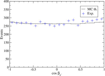
Figure 4: Angular distribution of the $e^{-}$ with respect to an axis orthogonal to the beam direction, in the $\tilde{\nu}_{e}$ rest frame.

4.2 Angular distributions of $\boldsymbol{\tilde{\chi}_{1}^{-}}$ decay products

The reconstruction of the chargino and sneutrino momenta allows for the determination of the chargino spin directions, which are $\vec{s}_{-}=\vec{P}_{\tilde{\chi}_{1}^{-}}$, $\vec{s}_{+}=-\vec{P}_{\tilde{\chi}_{1}^{+}}$ for $\tilde{\chi}_{1}^{-}$, $\tilde{\chi}_{1}^{+}$, respectively, with $\vec{P}_{\tilde{\chi}_{1}^{-}}$, $\vec{P}_{\tilde{\chi}_{1}^{+}}$ the chargino three-momenta in the $\tilde{\nu}_{e}$, $\tilde{\nu}_{e}^{*}$ rest frames. The knowledge of the chargino spin directions then makes it possible a precise study of its polarised differential decay widths. The analytical expressions for these quantities are rather lengthy [25]; however, the angular distribution of a single decay product in the $\tilde{\chi}_{1}^{-}$ rest frame can be cast in a compact form. Let us define $\theta_{\bar{f}}$, $\theta_{f^{\prime}}$, $\theta_{0}$ as the angles between the three-momenta of $\bar{f}=\bar{\nu},\bar{u},\bar{c}$, $f^{\prime}=\mu^{-},d,s$ and $\tilde{\chi}_{1}^{0}$ in the $\tilde{\chi}_{1}^{-}$ rest frame, respectively, and the $\tilde{\chi}_{1}^{-}$ spin (see Fig. 5). Analogous definitions hold for the $\tilde{\chi}_{1}^{+}$ decay products. Integrating all variables except $\theta_{\bar{f}}$, $\theta_{f^{\prime}}$ or $\theta_{0}$, the angular decay distributions read

$$\frac{1}{\Gamma^{(-)}}\frac{d\Gamma^{(-)}}{d\cos\theta_{\bar{f}}} = \frac{1+h_{\bar{f}}\cos\theta_{\bar{f}}}{2}\,,$$

$$\frac{1}{\Gamma^{(-)}}\frac{d\Gamma^{(-)}}{d\cos\theta_{f^{\prime}}} = \frac{1+h_{f^{\prime}}\cos\theta_{f^{\prime}}}{2}\,,$$

$$\frac{1}{\Gamma^{(-)}}\frac{d\Gamma^{(-)}}{d\cos\theta_{0}} = \frac{1+h_{0}^{(-)}\cos\theta_{0}}{2}\,,$$ (5)

with $\Gamma^{(-)}\equiv\Gamma(\tilde{\chi}_{1}^{-}\to\bar{f}f^{\prime}\tilde{\chi}_{1}^{0})$. The $h$ factors are called “spin analysing power” of the corresponding fermion $\bar{f}$, $f^{\prime}$, $\tilde{\chi}_{1}^{0}$, and are constants between $-1$ and $1$ which depend on the type of fermion and the supersymmetric scenario considered. For $\tilde{\chi}_{1}^{+}$ decays the angular distributions $d\Gamma^{(+)}/d\cos\theta_{f,\bar{f^{\prime}},0}$ are given by similar expressions with constants $h_{f}$, $h_{\bar{f}^{\prime}}$, $h_{0}^{(+)}$, which satisfy $h_{f}=-h_{\bar{f}}$, $h_{\bar{f}^{\prime}}=-h_{f^{\prime}}$, $h_{0}^{(+)}=-h_{0}^{(-)}$ if CP is conserved.

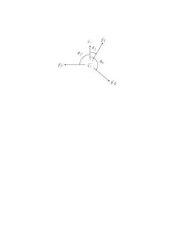
Figure 5: Definition of the polar angles $\theta_{\bar{f}}$, $\theta_{f^{\prime}}$ and $\theta_{0}$ in the decay of $\tilde{\chi}_{1}^{-}$.

The angular distribution of the muon resulting from $\tilde{\chi}_{1}^{-}$ decay is shown in Fig. 6. For $\cos\phi_{\mu^{-}}\simeq-1$ the muon is produced opposite to the $\tilde{\chi}_{1}^{-}$ momentum, then approximately parallel to the $e^{+}$ momentum (up to a Lorentz boost). Then, these events are suppressed by the requirement of lego-plot separation $\Delta R\geq 0.4$. With an accurate modelling of the real detector, all the $\cos\theta_{\mu^{-}}$ range could be eventually included in a fit to experimental data. In our study we restrict ourselves to the ranges where kinematical cuts do not alter the distributions. The fit to the data points (discarding the first three bins) gives $h_{\mu^{-}}=-0.270\pm 0.016$, in good agreement with the theoretical value $h_{\mu^{-}}=-0.252$.

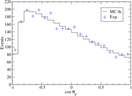
Figure 6: Angular distribution of the $\mu^{-}$ with respect to the $\tilde{\chi}_{1}^{-}$ spin, in the $\tilde{\chi}_{1}^{-}$ rest frame.

The study of quark angular distributions requires $c$ tagging to distinguish between the two quark jets. This reduces the signal by a factor of four, and thus decreases the statistical accuracy of the measurements. The angular distribution of the $s$ quark is presented in Fig. 7. The suppression around $\cos\theta_{s}\simeq-1$ is again caused by the requirement of lego-plot separation. The fit to the data points gives $h_{s}=-0.151\pm 0.020$, to be compared with the real value $h_{s}=-0.149$. The distribution of the $\bar{c}$ antiquark is presented in Fig. 8. In addition to the suppresion at $\cos\theta_{\bar{c}}\simeq-1$, we notice a decrease around $\cos\theta_{\bar{c}}\sim 1$, which is indirectly caused by the depression at $\cos\theta_{s}\simeq-1$. We thus discard the last seven bins for the fit to the distribution and obtain $h_{\bar{c}}=0.387\pm 0.044$, being the real value $h_{\bar{c}}=0.339$.

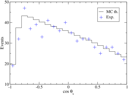
Figure 7: Angular distribution of the $s$ quark with respect to the $\tilde{\chi}_{1}^{-}$ spin, in the $\tilde{\chi}_{1}^{-}$ rest frame.

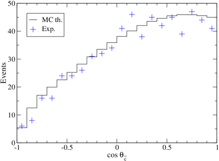
Figure 8: Angular distribution of the $\bar{c}$ antiquark with respect to the $\tilde{\chi}_{1}^{-}$ spin, in the $\tilde{\chi}_{1}^{-}$ rest frame.

As shown by these examples, the “spin analysing power” constants governing the angular distributions of $\tilde{\chi}_{1}^{-}$ are expected to be measured with an accuracy which ranges from 6% for $h_{\mu^{-}}$ to 13% for $h_{s}$. We note that the samples of “experimental measurements” generated have been chosen so that the total number of observed events is around $1\,\sigma$ away from the expected number, thus the difference between the measured and true values of the $h$ constants is due to statistics. The analysis of $\tilde{\chi}_{1}^{+}$ decays can be carried out analogously. However, it is interesting to point out that in CP-conserving scenarios the decays $\tilde{\chi}_{1}^{-}\to\bar{f}f^{\prime}\tilde{\chi}_{1}^{0}$, $\tilde{\chi}_{1}^{+}\to f\bar{f}^{\prime}\tilde{\chi}_{1}^{0}$ can be summed, substituting $\cos\theta_{\mu^{+},c,\bar{s}}\to-\cos\theta_{\mu^{-},\bar{c},s}$, improving the statistics by a factor $\sim\sqrt{2}$. Even in CP-violating scenarios this is likely to be a good approximation, because $h_{\mu^{-}}+h_{\mu^{+}}$, $h_{c}+h_{\bar{c}}$, $h_{s}+h_{\bar{s}}$ are negligible at the tree level, as will be shown in the next subsection, and get nonzero values only through higher order corrections.

4.3 CP violation in chargino decays

The construction of CP-violating observables involves the comparison of $\tilde{\chi}_{1}^{-}$ and $\tilde{\chi}_{1}^{+}$ decays. Under CP, the vectors in Fig. 5 transform to

$$\vec{s}_{-}\to\vec{s}_{+}\,,\quad\vec{p}_{\bar{f}}\to-\vec{p}_{f}\;,\quad\vec{p}_{f^{\prime}}\to-\vec{p}_{\bar{f}^{\prime}}\;,\quad\vec{p}_{\tilde{\chi}_{1}^{0}}\to-\vec{p}_{\tilde{\chi}_{1}^{0}}\;,$$ (6)

defined for the $\chi_{1}^{+}$ decay. Then, if we sum $\tilde{\chi}_{1}^{-}$ and $\tilde{\chi}_{1}^{+}$ decays the products

$$Q_{\mu} = \vec{s}_{\pm}\cdot\vec{p}_{\mu^{\pm}}\,,$$

$$Q_{c} = \vec{s}_{\pm}\cdot\vec{p}_{c(\bar{c})}\,,$$

$$Q_{s} = \vec{s}_{\pm}\cdot\vec{p}_{\bar{s}(s)}$$ (7)

are CP-odd. In hadronic decays an additional product $\vec{s}_{\pm}\cdot\vec{p}_{\tilde{\chi}_{1}^{0}}$ can be measured but it equals $-(Q_{c}+Q_{s})$. Since these products are even under naive T reversal, the CP-violating asymmetries

$$A_{X}=\frac{N(Q_{X}>0)-N(Q_{X}<0)}{N(Q_{X}>0)+N(Q_{X}<0)}\,,$$ (8)

with $X=\mu,c,s$ and $N$ standing for the number of events, are also T-even. Hence, they need the presence of absorptive CP-conserving phases in the amplitudes in order to be nonvanishing. In the processes under consideration these phases are generated at the tree level by intermediate particle widths, but they are extremely small, giving asymmetries $A_{X}\sim 10^{-3}$. At one loop level, these asymmetries can result from the interference between a dominant tree-level and a subleading one-loop diagram with a CP-conserving phase, and are expected to be very small as well.

Neglecting for the moment all particle widths (which are kept in all our numerical computations), the asymmetries $A_{X}$ vanish at the tree level. Using the fact that in this approximation the tree-level partial rates $\Gamma(\tilde{\chi}_{1}^{-}\to\bar{f}f^{\prime}\tilde{\chi}_{1}^{0})$ and $\Gamma(\tilde{\chi}_{1}^{+}\to f\bar{f}^{\prime}\tilde{\chi}_{1}^{0})$ are equal (because partial rate CP asymmetries are also T-even), these asymmetries are

$$A_{X}=\frac{h_{X}+h_{\bar{X}}}{4}\,.$$ (9)

Thus, $h_{\mu^{-}}+h_{\mu^{+}}$, $h_{c}+h_{\bar{c}}$, $h_{s}+h_{\bar{s}}$ vanish at the tree level if particle widths are neglected, and take values $O(10^{-3})$ (much smaller than the precision of the measurement of the individual constants) when particle widths are included.

A CP-odd, T-odd asymmetry can be built from the product

$$Q_{12}=\vec{s}_{\pm}\cdot\left(\vec{p}_{\bar{q}_{1}}\times\vec{p}_{q_{2}}\right)\,,$$ (10)

where $\vec{p}_{\bar{q}_{1}}$ and $\vec{p}_{q_{2}}$ are the momenta of the antiquark and quark resulting from the hadronic $\tilde{\chi}_{1}^{\pm}$ decay, respectively. (A triple product $\vec{s}_{\pm}\cdot(\vec{p}_{X_{1}}\times\vec{p}_{X_{2}})$, with $X_{1}=c,\bar{c}$, $X_{2}=\bar{s},s$ distinguished by quark flavour instead of baryon number, is CP-even.) The quark and antiquark are distinguished using $c$ tagging and looking at the charge of the muon, as explained in section 3. The CP asymmetry

$$A_{12}=\frac{N(Q_{12}>0)-N(Q_{12}<0)}{N(Q_{12}>0)+N(Q_{12}<0)}$$ (11)

can be sizeable already at the tree level, and without the need of interference between different Feynman diagrams. As discussed in section 2, in the SUSY scenario selected the $\tilde{\chi}_{1}^{-}$ decays are strongly dominated by diagram (a) in Fig. 3. A large triple-product CP asymmetry is possible because the polarised decay width for $\tilde{\chi}_{1}^{-}\to W^{-}\tilde{\chi}_{1}^{0}\to\bar{f}f^{\prime}\tilde{\chi}_{1}^{0}$ contains a term proportional to $\epsilon_{\mu\nu\rho\sigma}s_{-}^{\mu}\,P_{\bar{\chi}_{1}^{-}}^{\nu}\,P_{\bar{f}}^{\rho}\,P_{f^{\prime}}^{\sigma}\;m_{\tilde{\chi}_{1}^{0}}\;\mathrm{Im}\,O_{R}^{11}O_{L}^{11*}$, where $O_{L,R}^{11}$ denote the left- and right-handed parts of the (complex) $W\tilde{\chi}_{1}^{0}\tilde{\chi}_{1}^{-}$ coupling, respectively, and the momenta follow obvious notation. In the $\tilde{\chi}_{1}^{-}$ rest frame we have $P_{\bar{\chi}_{1}^{-}}=(\,m_{\tilde{\chi}_{1}^{-}},\vec{0}\,)$, $\vec{P}_{\bar{f}}=\vec{p}_{\bar{f}}$, $\vec{P}_{f^{\prime}}=\vec{p}_{f^{\prime}}$ and this term reduces to a triple product.

The theoretical value of $A_{12}$ as a function of $\phi_{1}$, taking $\phi_{\mu}=0$, is shown in Fig. 9 (a), where we observe that the asymmetry can reach values $O(0.1)$ for large phases $\phi_{1}\simeq 2$. For large $\phi_{\mu}$ values the asymmetry could be large too, as can be seen in Fig. 9 (b). However, for the range $|\phi_{\mu}|\lesssim 0.12$ (modulo $\pi$) allowed by EDM constraints the variation of $A_{12}$ is only between $\pm 0.01$.

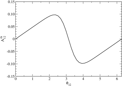
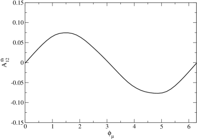
(a)	(b)

Figure 9: Theoretical value of $A_{12}$ as a function of $\phi_{1}$, for $\phi_{\mu}=0$ (a) and as a function of $\phi_{\mu}$, for $\phi_{1}=0$ (b).

We present in Fig. 10 the value of the asymmetry after signal reconstruction, including the corrections from ISR, beamstrahlung, etc. discussed in section 3. The shaded region represents the statistical error for one year of running with an integrated luminosity of 534 fb^-1. The variation of the cross section with $\phi_{1}$ is not relevant. In this plot we have chosen pairs of phases $(\phi_{1},\phi_{\mu})$ allowed by EDM constraints: for each $\phi_{1}$, we take a $\phi_{\mu}$ value, with $|\phi_{\mu}|\lesssim 0.12$, for which the neutralino and chargino contributions to the electron EDM cancel. Then, we calculate the asymmetry for this $(\phi_{1},\phi_{\mu})$ pair. (Several representative examples of these allowed pairs of phases are collected in Table 2.) The maximum differences in the asymmetry between taking $\phi_{\mu}=0$ and taking the $\phi_{\mu}$ values required by EDM constraints are of 10%, found for $\phi_{1}\sim 0,\pi$.

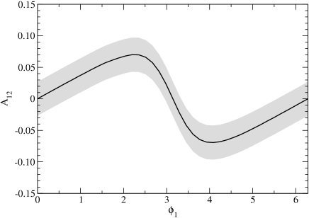
Figure 10: Asymmetry $A_{12}$ as a function of the phase $\phi_{1}$, for $\phi_{\mu}$ values fulfilling EDM constraints, as explained in the text. The shaded region represents the statistical error for one year of running.

5 Conclusions

In this paper we have shown that, in SUSY scenarios where the decays $\tilde{\nu}_{e}\to e^{-}\tilde{\chi}_{1}^{+}$, $\tilde{\nu}_{e}^{*}\to e^{+}\tilde{\chi}_{1}^{-}$ are kinematically allowed, sneutrino pair production provides a copious source of 100% polarised charginos, in which the kinematics of the process allows to reconstruct their four-momenta. The large cross section for the full process $e^{+}e^{-}\to\tilde{\nu}_{e}^{*}\tilde{\nu}_{e}\to e^{+}\tilde{\chi}_{1}^{-}\,e^{-}\tilde{\chi}_{1}^{+}\to e^{+}\bar{\nu}_{\mu}\mu^{-}\tilde{\chi}_{1}^{0}\,e^{-}q\bar{q}^{\prime}\tilde{\chi}_{1}^{0}$ (plus its charge conjugate) and the low backgrounds allow precise measurements of spin-related quantities like angular distributions and triple product CP-violating asymmetries.

The $e^{-}$ distribution in the $\tilde{\nu}_{e}$ rest frame shows that the $\tilde{\nu}_{e}$ decay is isotropic, what is a strong indication that sneutrinos are scalars. Since the spin of electrons is $1/2$, total angular momentum conservation implies that the charginos have half-integer spin, being $1/2$ the most obvious possibility. Angular distributions in $\tilde{\chi}_{1}^{-}$ rest frame allow to measure the values of the “spin analysing power” constants $h_{\mu^{-}}$, $h_{\bar{c}}$, $h_{s}$ controlling the angular distributions of its decay products, with a precision between 6% and 13% for only one year of running. Since the sums $h_{\mu^{-}}+h_{\mu^{+}}$, $h_{c}+h_{\bar{c}}$, $h_{s}+h_{\bar{s}}$ are zero if CP is conserved, and are expected to be small in CP-violating scenarios (even including radiative corrections), the data from $\tilde{\chi}_{1}^{+}$ decays could eventually be included in the analyses, improving the statistical precision.

Despite the fact that CP-violating phases could be detected in CP-conserving quantities [26], the direct observation of supersymmetric CP violation is extremely important. We have shown that in $\tilde{\chi}_{1}^{\pm}$ hadronic decays the CP-violating asymmetry in the product $\vec{s}_{\pm}\cdot(\vec{p}_{\bar{q}_{1}}\times\vec{p}_{q_{2}})$ is very sensitive to the phase of $M_{1}$, and can have values up to $A_{12}=0.07$ for $\phi_{1}\simeq 2$. Such asymmetry could be observed with $2.6\,\sigma$ statistical significance in one year of running. It is worth comparing this sensitivity with the ones obtained in other processes within the same SUSY scenario. In selectron cascade decays $\tilde{e}_{L}\to e\tilde{\chi}_{2}^{0}\to e\tilde{\chi}_{1}^{0}\mu^{+}\mu^{-}$, a CP asymmetry in the triple product $\vec{s}\cdot(\vec{p}_{\mu^{-}}\times\vec{p}_{\mu^{+}})$ can be built, with $\vec{s}$ the $\tilde{\chi}_{2}^{0}$ spin [27]. In $\tilde{\chi}_{1}^{0}\tilde{\chi}_{2}^{0}$ production $e^{+}e^{-}\to\tilde{\chi}_{1}^{0}\tilde{\chi}_{2}^{0}\to\tilde{\chi}_{1}^{0}\tilde{\chi}_{1}^{0}\ell^{+}\ell^{-}$, $\ell=e,\mu$, an analogous asymmetry in the product $\vec{p}_{e^{+}}\cdot(\vec{p}_{\ell^{-}}\times\vec{p}_{\ell^{+}})$ can be defined [10, 28]. The values of these asymmetries as a function of $\phi_{1}$ (including ISR, beamstrahlung, beam spread and detector effects, as well as backgrounds) are shown in Fig. 11 (adapted from Refs. [27, 10], where two years of running are considered instead of one). Comparing Figs. 10, 11 it is apparent that the observation of CP violating effects is much easier in sneutrino cascade decays. For large phases $\phi_{1}\simeq 2$ the statistical significance of the CP asymmetry $A_{12}$ is a factor of two larger than for the asymmetries in selectron cascade decays and neutralino pair production. Therefore, provided a good $c$ tagging efficiency is achieved, sneutrino cascade decays provide a much more sensitive tool to test CP violation in the neutralino sector than neutralino production and decay proceses.

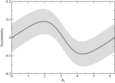
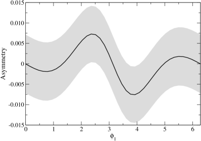
(a)	(b)

Figure 11: Triple product CP-violating asymmetries defined in (a) selectron cascade decays [27]; (b) $\tilde{\chi}_{1}^{0}\tilde{\chi}_{2}^{0}$ production [10], in the same SUSY scenario studied here. The shaded regions represent the statistical error for one year of running.

Acknowledgements

This work has been supported by the European Community’s Human Potential Programme under contract HTRN–CT–2000–00149 Physics at Colliders and by FCT through projects POCTI/FNU/43793/2002, CFIF–Plurianual (2/91) and grant SFRH/ BPD/12603/2003.

References

- [1] H. E. Haber and G. L. Kane, Phys. Rept. 117 (1985) 75
- [2] S. P. Martin, in “Perspectives on supersymmetry”, G. L. Kane (ed.), hep-ph/9709356
- [3] J. A. Aguilar-Saavedra et al. [ECFA/DESY LC Physics Working Group Collaboration], hep-ph/0106315
- [4] T. Ibrahim and P. Nath, Phys. Rev. D 57 (1998) 478 [Erratum-ibid. D 58 (1998) 019901, Erratum-ibid. D 60 (1999) 079903, Erratum-ibid. D 60 (1999) 019901]
- [5] T. Ibrahim and P. Nath, Phys. Rev. D 58 (1998) 111301 [Erratum-ibid. D 60 (1999) 099902]
- [6] M. Brhlik, G. J. Good and G. L. Kane, Phys. Rev. D 59 (1999) 115004
- [7] B. C. Allanach et al., in Proc. of the APS/DPF/DPB Summer Study on the Future of Particle Physics (Snowmass 2001) ed. N. Graf, Eur. Phys. J. C 25, 113 (2002) [eConf C010630, P125 (2001)]
- [8] S. Y. Choi, A. Djouadi, H. K. Dreiner, J. Kalinowski and P. M. Zerwas, Eur. Phys. J. C 7 (1999) 123
- [9] J. A. Aguilar-Saavedra and A. M. Teixeira, Nucl. Phys. B 675, 70 (2003)
- [10] J. A. Aguilar-Saavedra, Nucl. Phys. B 697, 207 (2004)
- [11] J. C. Romão, http://porthos.ist.utl.pt/romao/homepage/publications/mssm- model/mssm-model.ps
- [12] W. Porod, Comput. Phys. Commun. 153, 275 (2003)
- [13] R. Arnowitt, B. Dutta and Y. Santoso, Phys. Rev. D 64 (2001) 113010
- [14] K. Hagiwara et al., Particle Data Group, Phys. Rev. D66 (2002) 010001
- [15] T. Ibrahim and P. Nath, Phys. Rev. D 61 (2000) 093004
- [16] E. Murayama, I. Watanabe and K. Hagiwara, KEK report 91-11, January 1992
- [17] International Linear Collider Technical Review Committee 2003 Report, http://www.slac.stanford.edu/xorg/ilc-trc/2002/2002/report/03rep.htm
- [18] M. Skrzypek and S. Jadach, Z. Phys. C 49 (1991) 577
- [19] M. Peskin, Linear Collider Collaboration Note LCC-0010, January 1999
- [20] K. Yokoya and P. Chen, SLAC-PUB-4935. Presented at IEEE Particle Accelerator Conference, Chicago, Illinois, Mar 20-23, 1989
- [21] G. Alexander et al., TESLA Technical Design Report Part 4, DESY-01-011
- [22] R. Kleiss, W. J. Stirling and S. D. Ellis, Comput. Phys. Commun. 40 (1986) 359
- [23] S. M. Xella Hansen, C. Damerell, D. J. Jackson and R. Hawkings, Prepared for 5th International Linear Collider Workshop (LCWS 2000), Fermilab, Batavia, Illinois, 24-28 Oct 2000
- [24] S. Dittmaier and M. Roth, Nucl. Phys. B 642 (2002) 307
- [25] A. Djouadi, Y. Mambrini and M. Muhlleitner, Eur. Phys. J. C 20 (2001) 563
- [26] See for instance S. Y. Choi, A. Djouadi, M. Guchait, J. Kalinowski, H. S. Song and P. M. Zerwas, Eur. Phys. J. C 14 (2000) 535; S. Y. Choi, J. Kalinowski, G. Moortgat-Pick and P. M. Zerwas, Eur. Phys. J. C 22 (2001) 563 [Addendum-ibid. C 23 (2002) 769]; A. Bartl, S. Hesselbach, K. Hidaka, T. Kernreiter and W. Porod, Phys. Lett. B 573 (2003) 153; Phys. Rev. D 70 (2004) 035003; S. Y. Choi, M. Drees and B. Gaissmaier, Phys. Rev. D 70 (2004)
- [27] J. A. Aguilar-Saavedra, Phys. Lett. B 596 (2004) 247
- [28] See for instance S. Y. Choi, H. S. Song and W. Y. Song, Phys. Rev. D 61 (2000) 075004; A. Bartl, H. Fraas, S. Hesselbach, K. Hohenwarter-Sodek and G. Moortgat-Pick, JHEP 0408 (2004) 038