Measuring the MSSM Lagrangean

Abstract

At the LHC, it will be possible to investigate scenarios for physics beyond the Standard Model in detail. We present precise total and differential cross section predictions, based on Prospino2.0 and SMadGraph. We also show to what degree the structure of the weak–scale supersymmetric Lagrangean can be studied, based on LHC data alone or based on combined LHC and linear collider. Using Sfitter we correctly take into account experimental and theoretical errors. We make the case that a proper treatment of the error propagation is crucial for any analysis of this kind.

1 Introduction

In the near future, we expect the LHC experiments to unravel the mechanism of electroweak symmetry breaking and to search for new physics at the TeV scale. Over many years it has been established that for example supersymmetry can be discovered at the LHC, but also that the supersymmetric partner masses can be measured in cascade decays [1]. Mass measurements at the percent level, which can be supplemented with cross section [2] and branching fraction measurements [3] and with additional constraints like the dark matter relic density [4], will allow us to determine weak–scale Lagrangean parameters. Mass measurements at a future linear collider are typically at least one order of magnitude better than their LHC counterparts. More importantly, the sectors of the MSSM probed by the two machines nicely complement each other. A proper combined analysis [5] covers the entire MSSM spectrum and probes the complete weak–scale Lagrangean. It might even allow for an extrapolation to high scales [5, 6] where the structures of SUSY breaking become visible.

2 Next-to-leading order total cross sections

One basis for the inclusive search for supersymmetry at hadron colliders is precise predictions of all production cross sections. Similar to their Standard Model counterparts, SUSY-QCD cross sections are plagued by large theoretical errors, which can for example be observed in the renormalization and factorization scale variations. The Tevatron searches use next-to-leading order cross section predictions — until now unfortunately only ruling out parts of the SUSY parameter space. The large set of NLO cross sections at hadron colliders shown in Fig. 1 can be computed using the publicly available computer program Prospino2.0 [2]. In addition to squark and gluino production, pair production of neutralinos and charginos, which can decay into trilepton final states, has been included. Recently, we have seen that in split-supersymmetry models these Drell-Yan type processes together with the production of long-lived gluinos are the main SUSY signals at the LHC [7]. This feature is not limited to the extreme case of split supersymmetry. Cascade decays of squarks can already be decoupled for only slightly enhanced squark masses. A small hierarchy between gauginos and scalars appears for example in gravity mediated models with anomaly mediated gaugino masses, where this hierarchy alleviates the problems in the SUSY flavor sector [8].

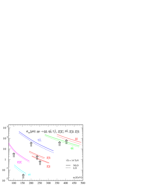
Figure 1: Leading order and NLO production cross sections at the LHC as a function of the average final state mass. The arrows indicate a typical SUGRA scenario.

In this paper we present new results for the associated production of charginos and neutralinos with gluinos [9, 10] and squarks [11]. After including these two classes of production processes, the list of cross sections available in Prospino2.0 is complete. The same way as for all processes shown in Fig. 1 we compute the complete SUSY-QCD corrections to the leading order processes $pp\to\tilde{q}\tilde{\chi}$ and $pp\to\tilde{g}\tilde{\chi}$. The results are available for the Tevatron and for the LHC. A technical complication is the correct subtraction of intermediate particles: the NLO contribution $pp\to\tilde{q}\tilde{\chi}$ includes an intermediate gluino with a subsequent decay $pp\to\tilde{g}\tilde{\chi}\to(q\tilde{q})\tilde{\chi}$, plus intermediate squark pair production $pp\to\tilde{q}^{*}\tilde{q}\to(q\tilde{\chi})\tilde{q}$. Of course, we could regularize this on-shell divergence using a Breit–Wigner propagator, but this would lead to double counting between $\tilde{q}\tilde{\chi}$ production, $\tilde{g}\tilde{\chi}$ production, and $\tilde{q}^{*}\tilde{q}$ production at the NLO level. To avoid any double counting in the combined inclusive SUSY samples, we instead subtract the on-shell squark contribution in the narrow width approximation [2]. This procedure is uniquely defined and allows us to naively add the different processes without having to worry about double counting at all, when including NLO effects to all $(2\to 2)$ production processes. In the top panel of Fig. 2 we see that this prescription leads to a smooth definition of the NLO cross section for the process $pp\to\tilde{q}\tilde{\chi}$ around the threshold $m_{\tilde{q}}=m_{\tilde{g}}$. Exactly the same way we subtract on-shell contributions $\tilde{g}\tilde{q}$ and $\tilde{q}\tilde{\chi}$ from the NLO contributions to $pp\to\tilde{g}\tilde{\chi}$, shown in the lower panel of Fig. 2. A small effect in the NLO cross section survives: above the threshold $m_{\tilde{g}}=m_{\tilde{q}}$ the NLO corrections decrease, because here the possibly on-shell intermediate state is actually on-shell and is therefore subtracted. Below threshold, these channels are still off-shell, but give a sizeable contribution to the cross section. Owed to the smaller collider energies, these thresholds are even smoother at the Tevatron.

Figure 2: Leading order and NLO production cross sections for the associated production of neutralinos with a gluino or a squark. The MSSM parameters are fixed to the SPS1a data point, and the squark mass or gluinos mass are varied independently in the graphs. The central parameters are $m_{\tilde{q}}=559$ GeV and $m_{\tilde{g}}=609$ GeV. The two lightest neutralino masses are 96 and 179 GeV.

3 Hard jet radiation in association with SUSY-QCD

Figure 3: The transverse momentum spectrum of the harder jet for squark and gluino production at the LHC, in association with two hard jets. The phase space for the jets is limited to $p_{T}>50$ GeV.

A large fraction of the weakly interacting SUSY partner spectrum appears as intermediate states in cascade decays of squarks and gluinos at the LHC. Because of the possibly large number of squarks and gluinos produced, the masses of these intermediate particles can be reconstructed from measured edges and thresholds in the decay cascades [1]. However, most of these edges and thresholds involve jets, and it is crucial to know which of the jets in the event come from: (i) the correct position in the cascade, (ii) another decay step in the cascade, or (iii) additional jet radiation in the event. As long as the mass differences between gluino, squarks and neutralinos are large, the cascade jets are required to be very hard. Simulating the additional jet with Pythia and Herwig implicitely assumes that all additional jets are fairly soft — therefore it is not surprising that they do not enter the analysis as candidates for cascade jets after the appropriate $p_{T}$ cuts.

A typical SUSY analysis might require three or more hard jets with a staggered $p_{T}$ cut of 150, 100, 50 GeV. We use SMadGraph [13] to compute the rate and the $p_{T}$ distributions for additional hard jets from the matrix element $pp\to\tilde{q}\tilde{g}+X$. We focus on two additional hard jets and limit their phase space to $p_{T}>50$ GeV, to allow them to enter the SUSY cascade analysis. Softer jets will increase the jet activity but will not appear as a candidate for a cascade jet. The suppression of the rate per additional hard jet of this kind is of the order of 1/2…2/3, so two additional jets reduce the total cross section for $\tilde{q}\tilde{g}$ to around 1/3 of the leading order cross section $pp\to\tilde{q}\tilde{g}$. This large factor is not unexpected, even though the NLO $K$ factor for this process at the LHC is well under control [2].

In Fig. 3 we show the $p_{T}$ spectrum of the harder of these two jets. It peaks around 100 GeV and decreases only very slowly. This means that we cannot apply a $p_{T}$ cut on jets to remove all jet radiation from the event sample. Instead, we will have to find ways to deal with this new combinatorical error from additional matrix element jets. While this jet radiation is not likely to become a problem for the discovery of SUSY or the discovery of cascade decays, it will soften the edges and thresholds and make it harder to fit the masses which appear inside the cascade. In particular at the LHC, all systematical and theoretical errors have to be taken into account to quantify the precision with which we can measure the SUSY particle masses and extract the weak-scale parameters in the MSSM Lagrangean — which we will discuss in the next section.

4 Extracting the MSSM Lagrangean

From a theorist’s point of view the measurement of masses, cross sections and branching fractions is only secondary. The relevant parameters we need to study the structure of weak-scale supersymmetry and possibly learn something about SUSY breaking are the parameters in the Lagrangean. The neutralino and chargino sector is a straightforward example: the two mass matrices are determined by the weak gaugino mass parameters $M_{1,2}$, the Higgsino mass parameter $\mu$, and by $\tan\beta$ (plus the Standard Model gauge sector). These four parameters can be extracted out of six mass measurements, but some of the mass measurements can also be traded for total cross section or asymmetry measurements at a future linear collider. Masses at a linear collider are the most precisely measured observables. Cross section measurements at the LHC are typically much weaker even than mass measurements at the LHC because of the large theoretical and systematical errors and are therefore not likely to be helpful for the parameter extraction..

As a simple starting point we assume gravity mediated supersymmetry breaking and fit the four model parameters listed in Tab. 1 to different sets of mass measurements. We use SuSpect [17] to compute the weak-scale MSSM parameters. The experimental errors on the mass measurements [18] represent cascade reconstruction at the LHC [1] and threshold scans at a linear collider [14]). The resulting absolute error on the high-scale model parameters is $\Delta^{(1)}$. Even though we assume a smeared set of measurements and the starting point of the fit is far away from the SPS1a scenario, the best fit values always agree with the ‘true’ values. Therefore, we omit the central values in the table. The theoretical error on the prediction of weak-scale masses from high-scale SUSY breaking can be estimated comparing different implementations of the renormalization group evolution [15] or comparing the two-loop results which we use with three-loop beta function running [16]. We use a relative error of $1\%$ for weakly interacting particles and $3\%$ for strongly interacting particles. The situation is more involved for the light Higgs mass, which can be computed using weak-scale input parameters. Here, the theoretical error consists of errors in the input parameters, dominantly the top mass uncertainty, and of unknown higher order effects. We assume a conservative error of 3 GeV altogether. When we add the theory errors and the experimental errors in squares they yield an error $\Delta^{(2)}$ on the extracted model parameters. We have checked that including theoretical errors not as Gaussian but without any preference for the known value, i.e. using a box shape, does not have a significant impact on our results.

As a cross check for the theoretical errors $\Delta^{(2)}$ we start with a mass spectrum from SuSpect, but fit the parameters using the SoftSusy renormalization group evolution [19]. The results are also shown in Tab. 1. We see that the central values of $m_{0},m_{1/2}$ and $\tan\beta$ lie within the error bands $\Delta^{(2)}$ obtained from the consistent SuSpect fit. Moreover, the errors of the consistent fit and the error on this combination of different implementations agree well. The central values for $A_{0}$ are in agreement with the error for the SuSpect fit, but they are sufficiently far away from the central value to illustrate that we cannot really determine $A_{0}$ from the set of masses, given our assumed theoretical errors.

If we step back and have a look at the parts of the spectrum we can observe at the LHC and at a linear collider we see that the linear collider misses the gluino and most of the squarks, while the LHC leaves wide open spaces in the neutralino and chargino spectrum. Considering gaugino mass unification as one of the most important predictions of gravity mediated SUSY we could say that a fit to the SUGRA parameters for either the LHC alone or a linear collider alone assumes SUGRA to then get out SUGRA. In contrast, combining the two sets of collider data nicely covers the entire MSSM spectrum and does allow us to actually test the SUGRA hypothesis.

However, it would be clearly preferable if we were able to measure weak-scale MSSM parameters, first confirm that some new physics looks like supersymmetry, and then extrapolate this established parameter set to some SUSY breaking scale. Even though there should be enough measurements, the extraction of the weak-scale Lagrangean is technically challenging: fitting a complex parameter space can become sensitive on the starting values, because of domain walls which the fit procedure cannot cross. It is not guaranteed that the best fit is always the global minimum. A method which is more likely to find the global minimum is a grid over the entire parameter space. However, if the parameter space is too big the resolution might not be sufficient to make sure the result is the best local minimum. Accounting for these respective shortcomings, Sfitter uses a combination of $\chi^{2}$ minimizations based on a grid and on a fit. In a subspace of the MSSM parameter space we use a grid and compute an appropriate subset of measurements (for example the neutralino–chargino sector). Starting from this minimum we fit first the remaining parameters to all measurements, and then the entire parameter set to make sure we find the correct local minimum. Recently proposed approaches like genetic algorithms or adaptive scanning methods [20] should allow us to further improve the coverage of the MSSM parameter space.

SPS1a	LHC			LC			LHC+LC
	$\Delta^{(1)}$	$\Delta^{(2)}$	SoftSusy	$\Delta^{(1)}$	$\Delta^{(2)}$	SoftSusy	$\Delta^{(1)}$	$\Delta^{(2)}$	SoftSusy
$m_{0}$	4.0	4.6	98 $\pm$ 4.6	0.09	0.70	99 $\pm$ 0.7	0.08	0.68	99 $\pm$0.8
$m_{1/2}$	1.8	2.8	253 $\pm$ 2.9	0.13	0.72	251 $\pm$ 0.7	0.11	0.67	251 $\pm$0.8
$\tan\beta$	1.3	3.4	11.6$\pm$ 3.4	0.14	0.49	10.1$\pm$ 0.5	0.14	0.49	10.1$\pm$0.6
$A_{0}$	31.8	50.5	14.7$\pm$ 14.2	4.43	13.9	-45 $\pm$ 16	4.23	13.1	-43 $\pm$ 17

Table 1: Fit results from Sfitter. For the consistent running the central values of the fit are omitted, because they match the SPS1a input within the given errors. The input values are 100 GeV, 250 GeV, 10 and -100 GeV for $m_{0},m_{1/2},\tan\beta$ and $A_{0}$. The experimental error alone leads to the quoted absolute error $\Delta^{(1)}$. After including a theoretical error on the masses, the error on the fitted values increases to $\Delta^{(2)}$. The last column assumes a spectrum created with SuSpect and a fit based on SoftSusy.

Results for the fit of the weak-scale MSSM Lagrangean we presented in Refs. [5, 21]. Details on the corresponding Fittino parameter determination are also available [22]. The main features for the SPS1a parameter point are: all three gaugino masses are covered by a combined LHC and linear collider analysis. The squark sector is determined by the LHC, a linear collider will likely be limited to the light stop. The slepton masses are well measured at the linear collider, while the LHC only sees a subset in the lepton invariant mass edge in cascade decays. The (heavy) Higgsinos are challenging for the linear collider and for the LHC, but their masses could be replaced by cross section measurements at the linear collider. The determination of the three heavy-flavor trilinear coupling parameters poses a serious problem: $A_{\tau}$ can be measured at a linear collider through a combination of stau mass and cross section measurements. $A_{b}$ might not be measured at either of the colliders, and for $A_{t}$ it is crucial to control the theoretical uncertainties of the light Higgs mass and the correlations with $\tan\beta$ and $\mu$. At the moment, the most important missing pieces are the stop sector at the LHC [23] and a direct measurement of $\tan\beta$ at either collider. For large values of $\tan\beta$ a measurement of $\tan\beta$ might be possible in the production of heavy Higgs bosons at the LHC, where the production rate is proportional to $\tan^{2}\beta$ [24]. These questions will be investigated when we extend our study beyond the low $\tan\beta$ parameter point SPS1a, at which point we will have to combine the SUSY-Higgs sector with the SUSY particle production.

5 Outlook

As part of the preparation for LHC data and its interpretation, there has been considerable progress in the collider phenomenology of new physics in general and of supersymmetry in particular. Beyond the discovery of supersymmetry we will for example be able to measure particle masses from the kinematics of cascade decays at the LHC. These measurements (combined with cross section and branching fraction measurements) can be used to determine a large fraction of weak-scale Lagrangean parameters. For all these measurements it is indispensable to reliably predict total and differential production cross sections. The proper tools Prospino2.0 and SMadGraph are (or will soon be) publicly available.

Moreover, we might well be able to use weak-scale measurements to extrapolate Lagrangean parameters to higher scales and probe supersymmetry breaking patterns. For this purpose, additional precision measurements from a future linear collider are particularly useful. It is absolutely crucial that we treat theoretical and experimental errors correctly in these renormalization group analyses. Using Sfitter (and Fittino) we show the promise of these approaches and also their limitation for example in the case of LHC data without any linear collider measurements.

I would like to thank David Rainwater, Tim Stelzer, Dirk Zerwas, Remi Lafaye and my coauthors on the Prospino publications. Without their collaboration the results presented in this article would simply not exist. Moreover, I am grateful to the DESY theory group for their kind hospitality while I wrote this contribution.

References

- [1] H. Bachacou, I. Hinchliffe and F. E. Paige, Phys. Rev. D 62, 015009 (2000); B. C. Allanach, C. G. Lester, M. A. Parker and B. R. Webber, JHEP 0009, 004 (2000).
- [2] see e.g. W. Beenakker, R. Höpker, M. Spira and P. M. Zerwas, Nucl. Phys. B 492, 51 (1997); W. Beenakker, M. Klasen, M. Krämer, T. Plehn, M. Spira and P. M. Zerwas, Phys. Rev. Lett. 83, 3780 (1999); Prospino2.0, http://pheno.physics.wisc.edu/plehn
- [3] M. Mühlleitner, A. Djouadi and Y. Mambrini, arXiv:hep-ph/0311167.
- [4] G. Polesello and D. R. Tovey, JHEP 0405, 071 (2004); for a recent review see also: G. Bertone, D. Hooper and J. Silk, arXiv:hep-ph/0404175.
- [5] R. Lafaye, T. Plehn and D. Zerwas, arXiv:hep-ph/0404282; http://sfitter.web.cern.ch; see also http://www-flc.desy.de/fittino
- [6] G. A. Blair, W. Porod and P. M. Zerwas, Eur. Phys. J. C 27, 263 (2003); B. C. Allanach, G. A. Blair, S. Kraml, H. U. Martyn, G. Polesello, W. Porod and P. M. Zerwas, arXiv:hep-ph/0403133.
- [7] W. Kilian, T. Plehn, P. Richardson and E. Schmidt, arXiv:hep-ph/0408088.
- [8] J. D. Wells, arXiv:hep-ph/0306127.
- [9] M. Spira, arXiv:hep-ph/0211145.
- [10] E. L. Berger, M. Klasen and T. M. P. Tait, Phys. Rev. D 62, 095014 (2000); erratum: Phys. Rev. D 67, 099901 (2003).
- [11] T. Plehn, talk at Tevatron University 2/14/2002, FNAL, U.S.
- [12] E. L. Berger, T. Han, J. Jiang and T. Plehn, arXiv:hep-ph/0312286.
- [13] G.-C. Cho, K. Hagiwara, J. Kanzaki, T. Plehn, D. Rainwater and T. Stelzer, in preparation.
- [14] J. A. Aguilar-Saavedra et al. [ECFA/DESY LC Physics Working Group Collaboration], arXiv:hep-ph/0106315.
- [15] B. C. Allanach, S. Kraml and W. Porod, JHEP 0303, 016 (2003).
- [16] I. Jack, D. R. T. Jones and A. F. Kord, arXiv:hep-ph/0408128.
- [17] A. Djouadi, J. L. Kneur and G. Moultaka, arXiv:hep-ph/0211331.
- [18] G. Weiglein et al., [LHC-LC study group report, in preparation], see also http://www.ippp.dur.ac.uk/georg/lhclc
- [19] B. C. Allanach, Comput. Phys. Commun. 143, 305 (2002).
- [20] B. C. Allanach, D. Grellscheid and F. Quevedo, JHEP 0407, 069 (2004); O. Brein, arXiv:hep-ph/0407340.
- [21] R. Lafaye, talk at ICHEP 2004, Bejing, China
- [22] P. Bechtle, preprint DESY-THESIS-2004-040
- [23] J. Hisano, K. Kawagoe and M. M. Nojiri, Phys. Rev. D 68, 035007 (2003).
- [24] B. C. Allanach et al. [Beyond the Standard Model Working Group Collaboration], arXiv:hep-ph/0402295; T. Plehn, Phys. Rev. D 67, 014018 (2003).