Application of chiral quark models to high-energy processes

Abstract

We discuss the predictions of chiral quark models for basic pion properties entering high-energy processes: generalized parton distributions (GPD’s) and unintegrated parton distributions (UPD’s). We stress the role of the QCD evolution, necessary to compare the predictions to data.

This is a very brief account of the talk based on Refs. [1, 2, 3, 4], where the reader is referred to for the details and references. We discuss the use of low-energy chiral quark models to compute low-energy matrix elements of hadronic operators appearing in high-energy processes, in particular we evaluate the generalized and unintegrated parton distributions (GPD’s and UPD’s) of the pion in the Nambu–Jona-Lasinio model and the Spectral Quark Model [4]. We carry on the QCD evolution, necessary when comparing the model predictions to data obtained at much higher scales.

The twist-2 GPD of the pion is defined as

$$H(x,\xi,-{\bf{\Delta}}_{\perp}^{2})=\int\frac{dz^{-}}{4\pi}e^{ixp^{+}z^{-}}\langle\pi^{+}(p^{\prime})|\bar{q}(0,-\frac{z^{-}}{2},0){\gamma^{+}}q(0,\frac{z^{-}}{2},0)|\pi^{+}(p)\rangle,$$

where the quark operator $q(z^{+},z^{-},z_{\perp})$ is on the light cone $z^{2}=0$ and the link operators $P\exp(ig\int_{0}^{z}dx^{\mu}A_{\mu})$ are implicitly present to ensure the gauge invariance (as usual we work in the light cone gauge $A_{+}=0$). A similar definition holds for the gluon distribution. In chiral quark models the evaluation of $H$ at the leading-$N_{c}$ (one-loop) level is straightforward. For the NJL model with the Pauli-Villars regularization we get

$$H_{\rm NJL}(x,0,-{\bf\Delta}_{\perp}^{2})=$$

$$\left[1+\frac{N_{c}M^{2}(1-x)|{\bf\Delta}_{\perp}|}{4\pi^{2}f_{\pi}^{2}s_{i}}\sum_{i}c_{i}\log\left(\frac{s_{i}+(1-x)|{\bf\Delta}_{\perp}|}{s_{i}-(1-x)|{\bf\Delta}_{\perp}|}\right)\right]\theta(x)\theta(1-x),$$

$$s_{i}=\sqrt{(1-x)^{2}{\bf\Delta}_{\perp}^{2}+4M^{2}+4\Lambda_{i}^{2}},$$

where $M$ is the constituent quark mass, $\Lambda_{i}$ are the PV regulators, and $c_{i}$ are suitable constants. For the simplest twice-subtracted case, explored below, one has, for any regulated function $f$, the operational definition

$$\sum_{i}c_{i}f(\Lambda_{i}^{2})=f(0)-f(\Lambda^{2})+\Lambda^{2}df(\Lambda^{2})/d\Lambda^{2}.$$

We use $M=280$ MeV and $\Lambda=871$ MeV, which yields the pion decay constant $f_{\pi}=93$ MeV. In the SQM the result is

$$H_{\rm SQM}(x,0,-{\bf\Delta}_{\perp}^{2})=\frac{m_{\rho}^{2}(m_{\rho}^{2}-(1-x)^{2}{\bf\Delta}_{\perp}^{2})}{(m_{\rho}^{2}+(1-x)^{2}{\bf\Delta}_{\perp}^{2})^{2}}\theta(x)\theta(1-x),$$

where $m_{\rho}$ is the mass of the $\rho$ meson. We check that the pion electromagnetic form factor is

$$F_{\rm SQM}(t)=\int_{0}^{1}dxH_{\rm SQM}(x,0,t)={\frac{m_{\rho}^{2}}{m_{\rho}^{2}+t}},$$

which is the built-in vector-meson dominance principle. For both models $F(0)=1$ and $H_{\rm SQM}(x,0,0)=\theta(x)\theta(1-x)$.

Our next goal is to compare the results to the data from transverse lattices [5]. We pass to the impact-parameter space via the Fourier-Bessel transformation, as well as carry the LO DGLAP perturbative QCD evolution from the low model scale $Q_{0}$=313 MeV [6] up to the scale of the data.

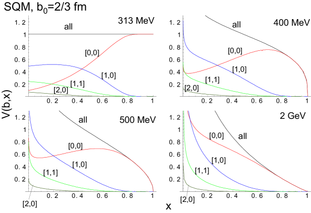
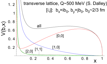
Figure 1: GPD of the pion in the impact-parameter space plotted as a function of the Bjorken $x$. Top: model for four momentum scales, from 313 MeV up to 2 GeV. Bottom: transverse lattice [5]. Numbers in brackets label the plaquette [1]. The qualitative agreement to the data is achieved at the scale of about 500 MeV.

The results are shown in Fig. 1. We note that while the results at $Q_{0}$ are completely different off the lattice data, when evolved to the scale of 500 MeV, corresponding to the lattice calculations, acquire a great resemblance to the data.

In the second part of this talk we discuss the leading-twist UPD’s of the pion, defined as

$$q(x,{k_{\perp}}) = \int\frac{dy^{-}d^{2}y_{\perp}}{16\pi^{3}}e^{-ixp^{+}y^{-}+i{k_{\perp}}\cdot y_{\perp}}\langle p\mid\bar{\psi}(0,y^{-},y_{\perp})\gamma^{+}\psi(0)\mid p\rangle,$$

and similarly for the gluon. An elementary one-quark-loop calculation in the NJL model with the PV regularization gives for $q$ and its Fourier-Bessel transform the result

$$q_{\rm NJL}(x,{k_{\perp}},Q_{0}) = \frac{\Lambda^{4}M^{2}N_{c}}{4f_{\pi}^{2}\pi^{3}\left({k_{\perp}^{2}}+M^{2}\right)\left({k_{\perp}^{2}}+\Lambda^{2}+M^{2}\right)^{2}}\theta(x)\theta(1-x)$$

$$F^{\rm NP}_{\rm NJL}({b}) = \frac{M^{2}N_{c}}{4f_{\pi}^{2}\pi^{2}}\left(2K_{0}({b}M)-2K_{0}({b}\sqrt{\Lambda^{2}+M^{2}})-\frac{{b}\Lambda^{2}K_{1}({b}\sqrt{\Lambda^{2}+M^{2}})}{\sqrt{\Lambda^{2}+M^{2}}}\right).$$

In SQM we find

$$q_{\rm SQM}(x,{k_{\perp}},Q_{0}) = \frac{6m_{\rho}^{3}}{\pi({k_{\perp}^{2}}+m_{\rho}^{2}/4)^{5/2}}\theta(x)\theta(1-x),$$

$$F^{\rm NP}_{\rm SQM}({b}) = \left(1+\frac{{b}m_{\rho}}{2}\right)\exp\left(-\frac{m_{\rho}{b}}{2}\right)$$

(the meaning of $b$ different here, it is the transverse coordinate conjugated to $k_{\perp}$). The above results are at the low model scale $Q_{0}$. Next, we evolve these UPD’s from $Q_{0}$ to high scales with the Kwieciński equations [2], obtained in the CCFM framework. The results are displayed in Fig. 2.

One may show several qualitative and quantitative results concerning UPD’s. At large $b$ they fall off exponentially and at large $k_{\perp}$ they fall off as a power law. Spreading with increasing $Q^{2}$ occurs, with $\langle k_{\perp}^{2}\rangle\sim Q^{2}\alpha_{S}(Q^{2})$. Also, asymptotic formulas at limiting cases may be explicitly given [2] which may be useful in checking numerical calculations of CCFM-type cascades [7].

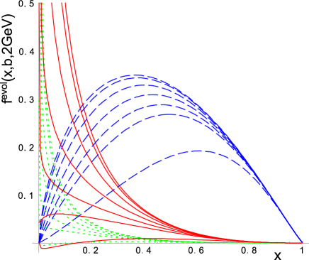
Figure 2: Valence quarks (dashed lines), sea quarks (dotted lines), and gluons (solid lines), for the transverse coordinate $b=0,1,2,3,4,5,$ and $10$ fm (bottom to top). Evolution with the Kwieciński equations from the model scale $Q_{0}$=313 MeV up to $Q=2$ GeV has been made.

Our basic conclusion is that chiral quark models may be used to provide GPD’s and UPD’s (also the pion distribution amplitude [3] not presented here) at the low model scale, $Q_{0}$. Upon evolution to higher scales, the agreement with the data (experimental or lattice) is very reasonable.

References

• [1] W. Broniowski and E. Ruiz Arriola, Phys. Lett. B 574, 57 (2003) [arXiv:hep-ph/0307198].
• [2] E. Ruiz Arriola and W. Broniowski, Phys. Rev. D 70, 034012 (2004) [arXiv:hep-ph/0404008].
• [3] E. Ruiz Arriola and W. Broniowski, Phys. Rev. D 66, 094016 (2002) [arXiv:hep-ph/0207266].
• [4] E. Ruiz Arriola and W. Broniowski, Phys. Rev. D 67, 074021 (2003) [arXiv:hep-ph/0301202].
• [5] S. Dalley, Phys. Lett. B 570, 191 (2003) [arXiv:hep-ph/0306121].
• [6] E. Ruiz Arriola, lectures given at 42nd Cracow School of Theoretical Physics, Flavor Dynamics, Zakopane, Poland, 31 May - 9 Jun 2002, Acta Phys. Polon. B 33 (2002) 4443.
• [7] H. Jung, Comput. Phys. Commun.  143, 100 (2002) [arXiv:hep-ph/0109102].