Universal phase between strong and EM interactions

It is shown that the experimental data of $\psi^{\prime}$ and $\psi^{\prime\prime}$ are consistent with a $-90^{\circ}$ phase between the strong and eletromagnetic decay amplitudes. The $e^{+}e^{-}\rightarrow\rho\pi$ measured at $\psi^{\prime\prime}$ is also consistent with the branching ratio predicted by Rosner’s scenario on $\rho\pi$ puzzle in charmonium physics. This scenario leads to a possible large charmless branching ratio in $\psi^{\prime\prime}$ decays.

1 Motivations

It has been known from experimental data that in two-body $J/\psi$ decays, the relative phase between the strong decay amplitude $a_{3g}$ and electromagnetic (EM) decay amplitude $a_{\gamma}$ is orthogonal for the decay modes $1^{+}0^{-}$ ($90^{\circ}$) [1], $1^{-}0^{-}$ $(106\pm 10)^{\circ}$ [2], $0^{-}0^{-}$ $(89.6\pm 9.9)^{\circ}$ [3], $1^{-}1^{-}$ $(138\pm 37)^{\circ}$ [4] and $N\overline{N}$ $(89\pm 15)^{\circ}$ [5].

It was argued [6] that this large phase follows from the orthogonality of three-gluon and one-photon virtual processes. The question arises: is this phase universal for quarkonium decays? How about $\psi^{\prime}$, $\psi^{\prime\prime}$ and $\Upsilon(nS)$ decays?

2 The phase between strong and EM amplitudes in $\psi^{\prime}$ decays

Recently, more $\psi^{\prime}$ data has been available. Most of the branching ratios are measured in $e^{+}e^{-}$ colliding experiments. For these experiments, there are three diagrams [7, 8] which contribute to the processes as shown in Fig. (3,3,3).

Figure 1: strong decay

Figure 2: EM decay

Figure 3: continuum

Until recently, the diagram in Fig. (3) has been neglected in the analysis of $\psi^{\prime}$ decays. But it leads to a continuum cross section and more important, it interferes with the amplitude of Fig. (3). So it affects the measured branching ratios significantly and alters the determination of the phase [8].

For the $e^{+}e^{-}\rightarrow 1^{-}0^{-}$ processes, the amplitudes depend on the three diagrams in the way [9]:

$$\begin{array}[]{ccl}A_{\omega\pi^{0}}&=&3(a_{\gamma}+a_{c})~{}~{},\\ A_{\rho\pi}&=&a_{3g}+a_{\gamma}+a_{c}~{}~{},\\ A_{K^{*+}K^{-}}&=&a_{3g}+\epsilon+a_{\gamma}+a_{c}~{}~{},\\ A_{K^{*0}\overline{K^{0}}}&=&a_{3g}+\epsilon-2(a_{\gamma}+a_{c})~{}~{}.\end{array}$$ (1)

where $\epsilon$ is the SU(3) symmetry breaking parameter. They can then be expressed as

$$\begin{array}[]{ccl}A_{\omega\pi^{0}}&=&[1+B(s)]\cdot{\cal F}_{\omega\pi^{0}}(s)~{}~{},\\ A_{\rho\pi}&=&[({\cal C}e^{i\phi}+1)B(s)+1]\cdot{\cal F}_{\omega\pi^{0}}(s)/3~{}~{},\\ A_{K^{*+}K^{-}}&=&[({\cal C}{\cal R}e^{i\phi}+1)B(s)+1]\cdot{\cal F}_{\omega\pi^{0}}(s)/3~{}~{},\\ A_{K^{*0}\overline{K^{0}}}&=&[({\cal C}{\cal R}e^{i\phi}-2)B(s)-2]\cdot{\cal F}_{\omega\pi^{0}}(s)/3~{}~{}.\\ \end{array}$$ (2)

where ${\cal R}=|(a_{3g}+\epsilon)/a_{3g}|$, $C=|a_{3g}/a_{\gamma}|$, and B(s) ≡3sΓee/αs-M2+iMΓt  . On top of the resonance, $B(s)=-i3B_{ee}/\alpha$ with phase of $-90^{\circ}$. If $\phi$ which is the phase between $a_{3g}$ and $a_{\gamma}$ is $-90^{\circ}$, then the relative phase between $a_{3g}$ and $a_{c}$ is $180^{\circ}$ for $\rho\pi$ and $K^{*+}K^{-}$, but $0^{\circ}$ for $K^{*0}\overline{K^{0}}$. The interference pattern due to this phase explains the small signal of $\rho\pi$ and $K^{*+}K^{-}$ but large signal of $K^{*0}\overline{K^{0}}$ observed by BES and CLEOc at $\psi^{\prime}$ [10, 11]. We suggest that in $\psi^{\prime}\rightarrow VP$ decays, the strong and EM amplitudes are still orthogonal and the sign of the phase must be negative [12].

For $\psi^{\prime}\rightarrow PP$ decays, the calculation [13] compared with the BES measurement of $B(\psi^{\prime}\rightarrow K^{0}_{S}K^{0}_{L})$ [14], leads to the conclusion that the phase between strong and EM amplitudes is either $(-82\pm 29)^{\circ}$ or $(121\pm 27)^{\circ}$.

3 $\psi^{\prime\prime}\rightarrow\rho\pi$ and Rosner’s scenario on $\rho\pi$ puzzle

As we turn to such phase in $\psi^{\prime\prime}$ decays, we get an extra prize which is the solution of the long-lasting $\rho\pi$ puzzle in charmonium decays. First we must digress to Rosner’s scenario.

While $\rho\pi$ has the largest branching ratio among the hadronic final states in $J/\psi$ decays, the same mode was not found in $\psi^{\prime}$ decays for a long time (recently, BES and CLEOc report its branching ratio at the order of $10^{-5}$ [10, 11]). Rosner proposed that this is due to the mixing between $\psi(2^{3}S_{1})$ and $\psi(1^{3}D_{1})$ states [15]:

$$\langle\rho\pi|\psi^{\prime}\rangle=\langle\rho\pi|2^{3}S_{1}\rangle\cos\theta-\langle\rho\pi|1^{3}D_{1}\rangle\sin\theta~{},$$

$$\langle\rho\pi|\psi^{\prime\prime}\rangle=\langle\rho\pi|2^{3}S_{1}\rangle\sin\theta+\langle\rho\pi|1^{3}D_{1}\rangle\cos\theta~{},$$

where $\theta=12^{\circ}$ is the mixing angle [15]. The missing of $\rho\pi$ in $\psi^{\prime}$ decay is due to the cancellation of the two terms in $\langle\rho\pi|\psi^{\prime}\rangle$. This scenario is simple, and it predicts with little uncertainty that ${\cal B}_{\psi^{\prime\prime}\rightarrow\rho\pi}=(6.8\pm 2.3)\times 10^{-4}~{}~{},$ or

$$\sigma^{Born}_{e^{+}e^{-}\rightarrow\psi^{\prime\prime}\rightarrow\rho\pi}=(7.9\pm 2.7)\mbox{pb}$$ (3)

with BES latest result on ${\cal B}(J/\psi\rightarrow\rho\pi)$ [16].

On the other hand, using CLEOc measurement of $e^{+}e^{-}\rightarrow\rho\pi$ at 3.67GeV [11], scaled to 3.77GeV according to $1/s^{2}$, we obtain

$$\sigma^{Born}_{e^{+}e^{-}\rightarrow\gamma^{*}\rightarrow\rho\pi}(3.770GeV)=(7.5\pm 1.8)\mbox{pb}.$$ (4)

The Born cross sections in Eqs.(3) and (4) are comparable. The question arises: how do they interfere?

As a matter of fact, MARK-III measured this cross section at $\psi^{\prime\prime}$ peak, and gave [17]

$$\sigma_{e^{+}e^{-}\rightarrow\rho\pi}(3.770GeV)<6.3\mbox{pb},$$ (5)

which is already smaller than the continuum cross section in Eq.(4). We expect BES and CLEOc to bring this value further down. This means [18]:

• There must be destructive interference between resonance and continum, i.e. the phase between the strong and EM amplitudes is again $-90^{\circ}$.

• ${\cal B}(\psi^{\prime\prime}\rightarrow\rho\pi)\approx(6\sim 7)\times 10^{-4}$, i.e. Rosner’s scenario gives correct prediction!

If we scan $\psi^{\prime\prime}$, we shall find the cross sections of $e^{+}e^{-}\rightarrow\rho\pi$ and $e^{+}e^{-}\rightarrow K^{*0}\overline{K^{0}}+c.c.$ versus energy like the curves in Fig.(4). In the figure, the hatched area is due to an unknown phase between the $2^{3}S_{1}$ and $1^{3}D_{1}$ matrix elements [18]. The $K^{*+}K^{-}+c.c.$ cross section is similar to $\rho\pi$.

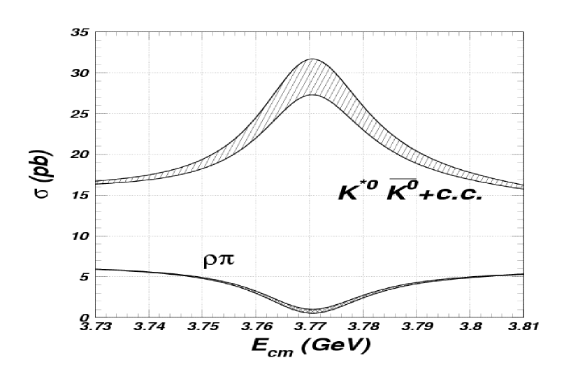
Figure 4: The $e^{+}e^{-}\rightarrow\rho\pi$ and $e^{+}e^{-}\rightarrow K^{*0}\overline{K^{0}}+c.c.$ cross sections around $\psi^{\prime\prime}$ peak, assuming Rosner’s scenario and $-90^{\circ}$ phase between strong and EM amplitudes. Hatched area is due to an unknown phase between the $2^{3}S_{1}$ and $1^{3}D_{1}$ matrix elements.

4 The phase in $\Upsilon$ decays

CLEO observed $K^{*}K$ but not $\rho\pi$ in $\Upsilon$ decays [19]. It can be due to the same interference pattern. We suppose the $K^{*}K$ signal in CLEO observation is mainly $K^{*0}\overline{K^{0}}$, not $K^{*+}K^{-}$.

5 Rosner’s scenario and enhanced modes in $\psi^{\prime}$ decays

Recently BES found modes which are enhanced in $\psi^{\prime}$ decays relative to $J/\psi$. One of them is $K^{0}_{S}K^{0}_{L}$: ${\cal B}(J/\psi\rightarrow K^{0}_{S}K^{0}_{L})=(1.82\pm 0.04\pm 0.13)\times 10^{-4}$ and ${\cal B}(\psi(2S)\rightarrow K^{0}_{S}K^{0}_{L})=(5.24\pm 0.47\pm 0.48)\times 10^{-5}$ with $Q_{h}=(28.8\pm 3.7)\%$ versus 12% rule. If such enhancement is due to the mixing of $2^{3}S_{1}$ and $1^{3}D_{1}$ states, then we expect [20] $(1.2\pm 0.7)\times 10^{-6}\leq{\cal B}(\psi(3770)\rightarrow K^{0}_{S}K^{0}_{L})\leq(3.8\pm 1.1)\times~{}10^{-5}$. Here the range is due to an unknown phase between $\langle K^{0}_{S}K^{0}_{L}|2^{3}S_{1}\rangle$ and $\langle K^{0}_{S}K^{0}_{L}|1^{3}D_{1}\rangle$. If this phase is 0, then the prediction is at the upper bound.

Currently BES gives an upper limit [21] ${\cal B}(\psi^{\prime\prime}\rightarrow K^{0}_{S}K^{0}_{L})<2.1\times 10^{-4}$. We expect CLEOc to give the branching ratio.

6 $\psi^{\prime\prime}$ decays to charmless final states

It has been noticed that there is hadronic excess in $\psi^{\prime}$ decays which has no parallel in $\Upsilon$ physics [1, 22]:

$$Q_{1}=\frac{{\cal B}(\psi^{\prime}\rightarrow ggg+\gamma gg)}{{\cal B}(J/\psi\rightarrow ggg+\gamma gg)}=(26.0\pm 3.5)\%~{}~{}$$ (6)

versus 12% rule. It indicates that most of the $\psi^{\prime}$ partial widths via gluons go to the final states which are enhanced in $\psi^{\prime}$ decays. Now we do not know what these final states are. The question arises: what is their branching ratio in $\psi^{\prime\prime}$ decays? There has been experimental indication that $\psi^{\prime\prime}$ has a substantial charmless branching ratio, although it comes with large uncertainties. This was addressed again recently [23]. So let us estimate the possible combined branching ratio of these final states in $\psi^{\prime\prime}$ decays.

We define the suppression and enhancement factor [23]

$$Q(f)\equiv\frac{\Gamma(\psi^{\prime}\rightarrow f)}{\Gamma(J/\psi\rightarrow f)}\frac{\Gamma(J/\psi\rightarrow e^{+}e^{-})}{\Gamma(\psi^{\prime}\rightarrow e^{+}e^{-})}~{}.$$ (7)

$Q(f)<1$ means the final state $f$ is suppressed in $\psi^{\prime}$ decays relative to $J/\psi$; $Q(f)>1$ means it is enhanced; $Q(f)=1$ means it observes the 12% rule.

In the $2S-1D$ mixing scheme, for any final state, its partial width in $\psi^{\prime\prime}$ decay can be related to its partial widths in $J/\psi$ and $\psi^{\prime}$ decay with an unknown parameter which is the relative phase between the matrix elements $\langle f|2^{3}S_{1}\rangle$ and $\langle f|1^{3}D_{1}\rangle$. This unknown phase constrains the predicted $\Gamma(\psi^{\prime\prime}\rightarrow f)$ in a finite range. We calculate $R_{\Gamma}\equiv\Gamma(\psi^{\prime\prime}\rightarrow f)/\Gamma(J/\psi\rightarrow f)$ as a function of $Q(f)$ and plot it in Fig. (5). In the figure the solid contour corresponds to the solution with no extra phase between $\langle f|2^{3}S_{1}\rangle$ and $\langle f|1^{3}D_{1}\rangle$; dashed contour corresponds to the solution with a relative negative sign between $\langle f|2^{3}S_{1}\rangle$ and $\langle f|1^{3}D_{1}\rangle$; the hatched area corresponds to the solution with other non-zero phase between $\langle f|2^{3}S_{1}\rangle$ and $\langle f|1^{3}D_{1}\rangle$. From Fig. (5) we see that those final states with large $Q(f)$ may contribute a combined large branching ratio in $\psi^{\prime\prime}$ decays.

Figure 5: $R_{\Gamma}$ as a function of $Q(f)$. The solid contour corresponds to no extra phase between the matrix elements $\langle f|2^{3}S_{1}\rangle$ and $\langle f|1^{3}D_{1}\rangle$; dashed contour corresponds to a relative negative sign between the matrix elements; the hatched area corresponds to other non-zero phase between the marix elements.

The decays of $J/\psi$ and $\psi^{\prime}$ are classified into gluonic decays ($ggg$), electromagnetic decays ($\gamma^{*}$), radiatve decays into light hadrons ($\gamma gg$), and OZI allowed decays into lower mass charmonium states. By subtracting the second to fourth classes, we obtain ${\cal B}(J/\psi\rightarrow ggg)\approx(69.2\pm 0.6)\%$ and ${\cal B}(\psi^{\prime}\rightarrow ggg)\approx(18.0\pm 2.4)\%$. Among these final states, we know that VP and VT final states have $Q(f)<1$, and $N\bar{N}$ have $Q(f)\approx 1$. Together they consist 5.4% of $J/\psi$ decays and $1.8\times 10^{-3}$ of $\psi^{\prime}$ decays. We subtract their branching ratios from the total branching ratio of gluonic decays of $J/\psi$ and $\psi^{\prime}$. The remaining 63.8% of $J/\psi$ decay and 17.8% of $\psi^{\prime}$ decay which go to final states through $ggg$ either have $Q(f)>1$ or $Q(f)$ unknown. On the average these final states have $Q(rem)\approx 2.19$. For this $Q$ value, the maximum $R_{\Gamma}$ is 51.6. So the maximum partial width of these final states in $\psi^{\prime\prime}$ is $\Gamma_{tot}(J/\psi)\times 63.8\%\times 51.6$ which is 3.0MeV, or 13% of the total $\psi^{\prime\prime}$ decay.

The above maximum value of $R_{\Gamma}$ comes if there is no extra phase between $\langle f|2^{3}S_{1}\rangle$ and $\langle f|1^{3}D_{1}\rangle$. There are reasons to assume that this is the case: (1) in the matrix element of $\langle\rho\pi|\psi^{\prime}\rangle$, there is almost complete cancellation between the contributions from $2^{3}S_{1}$ and $1^{3}D_{1}$ matrix elements, so the phase between them must close to 0; (2) if the phase between the strong and EM ampitudes is universal, then there is no extra phase between $2^{3}S_{1}$ and $1^{3}D_{1}$ matrix elements due to strong interactions, since there is no extra phase between the two matrix elements due to EM interactions, as in the calculations of leptonic decays. So we suppose that the partial widths of these final states are at the maximum values calculated here.

The calculations here take the averaged $Q(f)$ so serve as a rough estimation. The exact charmless partial width should be the sum of individual final states which in general have different values of $Q(f)$. But at present, experiments do not provide enough informationm to conduct such calculation. Nevertheless, the calculation here shows that a large charmless branching ratio in $\psi^{\prime\prime}$ decays, e.g. more than 10%, is not a surprise. It is well explained in the $2S-1D$ mixing scenario. Measuring the charmless branching ratio of $\psi^{\prime\prime}$ decays, both inclusive and exclusive, should be a primary physics goal for BES and CLEOc.

7 Summary

The $\psi^{\prime}\rightarrow 1^{-}0^{-}$ and $0^{-}0^{-}$ data collected in $e^{+}e^{-}$ experiments are consistent with a $-90^{\circ}$ phase between strong and electromagnetic interactions. This phase also holds in OZI suppressed decays of $\psi^{\prime\prime}$. This is from the measured $\rho\pi$ cross sections at $\psi^{\prime\prime}$ and 3.67GeV. At the same time these measurements give ${\cal B}(\psi^{\prime\prime}\rightarrow\rho\pi)$ which agrees with the prediction by Rosner in his scenario explaining the $\rho\pi$ puzzle. This scenario would be further supported if the large charmless branching ratio in $\psi^{\prime\prime}$ decays is confirmed by experiments.

References

[1]
M. Suzuki, Phys. Rev. D 63, 054021 (2001).
[2]
R. M. Bautrusatis et al., Phys. Rev. D 32, 2883 (1985);
D. Coffman et al., Phys. Rev. D 38, 2695 (1988);
L. Köpke and N. Wermes, Phys. Rep. 174, 67 (1989);
J. Jousset et al.,
Phys. Rev. D 41, 1389 (1990);
G. López Castro et al., in CAM-94, Cancum, Mexico,
edited by A. Zepeda, AIP Conf. Proc. 342 (AIP, New York, 1995), p.441;
A. Bramon, R. Escribano and M. D. Scadron, Phys. Lett. B 403,
339 (1997);
M. Suzuki, Phys. Rev. D 58, 111504 (1998);
N. N. Achasov and V. V. Gubin, Phys. Rev. D 61, 117504 (2000).
[3] L. Köpke and N. Wermes in Ref [2];
G. López Castro et al. in Ref [2];
M. Suzuki, Phys. Rev. D 60, 051501 (1999).
[5]
A. Antonelli, Phys. Lett. B 301, 317 (1993);
G. López Castro et al. in Ref [2];
R. Baldini, C. Bini and E. Luppi, Phys. Lett. B 404, 362 (1997).
FENICE Collaboration, R. Baldini, et al.
Phys. Lett. B 444, 111 (1998);
[6] J. M. Gérard and J. Weyers,
Phys. Lett. B 462, 324 (1999).
[7] S. Rudaz, Phys. Rev. D 14, 298 (1976);
[8]P. Wang, C. Z. Yuan, X. H. Mo and D. H. Zhang,
Phys. Lett. B 593, 89 (2004).
[9]H. E. Haber and J. Perrier, Phys. Rev. D 32, 2961 (1985).
[10]BES Collaboration, Y. S. Zhu, hep-ph/0407037, hep-ph/0408047.
[11]CLEO Collaboration, N. E. Adam et al., hep-ex/0407028.
[12] P. Wang, C. Z. Yuan, X. H. Mo,
Phys. Rev. D 69, 057502 (2004).
[13]C. Z. Yuan, P. Wang, X. H. Mo,
Phys. Lett. B 567, 73 (2003).
[14]BES Collaboration, J. Z. Bai et al.,
Phys. Rev. Lett. 92, 052001 (2004).
[15]J. L. Rosner, Phys. Rev. D 64 094002 (2001).
[16]BES Collaboration, M. Ablikim et al.,
Phys. Rev. D 70 012005 (2004).
[17] Yanong Zhu, Ph. D. thesis
California Institute of Technology, 1988,
Caltech Report No. CALT-68-1513;
W. A. Majid, Ph. D. thesis)
University of Illinois, 1993, UMI-94-11071-mc.
[18]P. Wang, C. Z. Yuan and X. H. Mo,
Phys. Lett. B 574, 41 (2003).
[19]CLEO Collaboration,
S. A. Dytman et al., hep-ex/0307035.
[20]P. Wang, C. Z. Yuan and X. H. Mo,
Phys. Rev. D 70 077505 (2004).
[21]BES Collaboration, M. Ablikim et al.,
Phys. Rev. D 70 077101 (2004).
[22] Y. F. Gu and X. H. Li, Phys. Rev. D 63 114019 (2001).