Recently, two of us (AD, DL) proposed a method for extracting the CP phase $\gamma$ from measurements of $B_{d}^{0}(t)\rightarrow D^{(*)+}D^{(*)-}$ and $B_{d}^{0}\rightarrow D_{s}^{(*)+}D^{(*)-}$ decays [1]. The technique is quite straightforward. Consider the pseudoscalar-pseudoscalar (PP) decay $B_{d}^{0}\rightarrow D^{+}D^{-}$. The amplitude for this decay receives several contributions, described by tree, exchange, ${\bar{b}}\rightarrow{\bar{d}}$ penguin and color-suppressed electroweak penguin diagrams [2]:

$$A^{D} = (T+E+P_{c})\,V_{cb}^{*}V_{cd}+P_{u}\,V_{ub}^{*}V_{ud}+(P_{t}+P_{\scriptscriptstyle EW}^{C})\,V_{tb}^{*}V_{td}$$ (1)

$$= (T+E+P_{c}-P_{t}-P_{\scriptscriptstyle EW}^{C})\,V_{cb}^{*}V_{cd}+(P_{u}-P_{t}-P_{\scriptscriptstyle EW}^{C})\,V_{ub}^{*}V_{ud}$$

$$\equiv {\cal A}_{ct}\ e^{i\delta^{ct}}+{\cal A}_{ut}\ e^{i\gamma}e^{i\delta^{ut}}~{}.$$

Here, ${\cal A}_{ct}\equiv|(T+E+P_{c}-P_{t}-P_{\scriptscriptstyle EW}^{C})V_{cb}^{*}V_{cd}|$, ${\cal A}_{ut}\equiv|(P_{u}-P_{t}-P_{\scriptscriptstyle EW}^{C})V_{ub}^{*}V_{ud}|$, $P_{i}$ is the ${\bar{b}}\rightarrow{\bar{d}}$ penguin amplitude with an internal $i$-quark, and we have explicitly written out the strong phases $\delta^{ct}$ and $\delta^{ut}$, as well as the weak phase $\gamma$. The second line is obtained by using the unitarity of the CKM matrix, $V_{ub}^{*}V_{ud}+V_{cb}^{*}V_{cd}+V_{tb}^{*}V_{td}=0$, to eliminate the $V_{tb}^{*}V_{td}$ term. The amplitude ${\bar{A}}^{D}$ for the decay ${\bar{B}}_{d}^{0}\rightarrow D^{+}D^{-}$ can be obtained from the above by changing the signs of the weak phases.

There are three observables which can be obtained from a time-dependent measurement of this decay: $B$ (the branching ratio), $a_{dir}$ (the direct CP asymmetry) and $a_{indir}$ (the indirect CP asymmetry). In terms of the above parameters, these can be written

$$B \equiv \frac{1}{2}\left(|A^{D}|^{2}+|{\bar{A}}^{D}|^{2}\right)={\cal A}_{ct}^{2}+{\cal A}_{ut}^{2}+2{\cal A}_{ct}{\cal A}_{ut}\cos\delta\cos\gamma~{},$$

$$a_{dir} \equiv \frac{1}{2}\left(|A^{D}|^{2}-|{\bar{A}}^{D}|^{2}\right)=-2{\cal A}_{ct}{\cal A}_{ut}\sin\delta\sin\gamma~{},$$ (2)

$$a_{indir} \equiv {\rm Im}\left(e^{-2i\beta}{A^{D}}^{*}{\bar{A}}^{D}\right)$$

$$= -{\cal A}_{ct}^{2}\sin 2\beta-2{\cal A}_{ct}{\cal A}_{ut}\cos\delta\sin(2\beta+\gamma)-{\cal A}_{ut}^{2}\sin(2\beta+2\gamma)~{},$$

where ${\delta}\equiv{\delta}^{ut}-{\delta}^{ct}$. Here, $\beta$ is the phase of $B_{d}^{0}$–${\bar{B}}_{d}^{0}$ mixing, which has been measured in the CP asymmetry in $B_{d}^{0}(t)\rightarrow J/\psi K_{\scriptscriptstyle S}$ [3]. However, these observables still depend on four unknown theoretical parameters: the two magnitudes ${\cal A}_{ct}$ and ${\cal A}_{ut}$, one relative strong phase ${\delta}$, and the weak phase $\gamma$. We therefore have three observables, but four theoretical unknowns. Thus, in order to obtain weak phase information, it is necessary to add some theoretical input [4].

This input comes from the decay $B_{d}^{0}\rightarrow D_{s}^{+}D^{-}$, which receives tree, ${\bar{b}}\rightarrow{\bar{s}}$ penguin and color-suppressed electroweak penguin contributions [2]:

$$A^{D_{s}} = (T^{\prime}+P^{\prime}_{c})\,V_{cb}^{*}V_{cs}+P^{\prime}_{u}\,V_{ub}^{*}V_{us}+(P^{\prime}_{t}+P_{\scriptscriptstyle EW}^{\prime C})\,V_{tb}^{*}V_{ts}$$ (3)

$$= (T^{\prime}+P^{\prime}_{c}-P^{\prime}_{t}-P_{\scriptscriptstyle EW}^{\prime C})\,V_{cb}^{*}V_{cs}+(P^{\prime}_{u}-P^{\prime}_{t}-P_{\scriptscriptstyle EW}^{\prime C})\,V_{ub}^{*}V_{us}$$

$$\approx (T^{\prime}+P^{\prime}_{c}-P^{\prime}_{t}-P_{\scriptscriptstyle EW}^{\prime C})\,V_{cb}^{*}V_{cs}\equiv{\cal A}_{ct}^{\prime}e^{i\delta^{\prime ct}}~{}.$$

(The primes on the amplitudes indicate a ${\bar{b}}\rightarrow{\bar{s}}$ transition.) Here, the last line arises from the fact that $\left|{V_{ub}^{*}V_{us}/V_{cb}^{*}V_{cs}}\right|\simeq 2\%$, so that the piece proportional to $V_{ub}^{*}V_{us}$ is negligible. The measurement of the total rate for $B_{d}^{0}\rightarrow D_{s}^{+}D^{-}$ therefore yields ${\cal A}_{ct}^{\prime}$.

We now make the SU(3) flavour assumption that

$$\Delta\equiv{\sin\theta_{c}\,{\cal A}_{ct}^{\prime}\over{\cal A}_{ct}}={\sin\theta_{c}|(T^{\prime}+P^{\prime}_{c}-P^{\prime}_{t}-P_{\scriptscriptstyle EW}^{\prime C})V_{cb}^{*}V_{cs}|\over|(T+E+P_{c}-P_{t}-P_{\scriptscriptstyle EW}^{C})V_{cb}^{*}V_{cd}|}=1~{},$$ (4)

where $\sin\theta_{c}$ is the Cabibbo angle. With this assumption, the knowledge of ${\cal A}_{ct}^{\prime}$ can be used to give us ${\cal A}_{ct}$. This in turn means that the three observables in $B_{d}^{0}\rightarrow D^{+}D^{-}$ depend on only three theoretical unknowns: ${\cal A}_{ut}$, $\delta$, and $\gamma$. We can therefore now solve for $\gamma$ (up to discrete ambiguities).

The explicit solution for $\gamma$ is as follows. We introduce a fourth (non-independent) observable, $a_{\scriptscriptstyle R}$:

$$a_{\scriptscriptstyle R} \equiv {\rm Re}\left(e^{-2i\beta}{A^{D}}^{*}{\bar{A}}^{D}\right)=B^{2}-a_{dir}^{2}-a_{indir}^{2}$$ (5)

$$= {\cal A}_{ct}^{2}\cos 2\beta+2{\cal A}_{ct}{\cal A}_{ut}\cos\delta\cos(2\beta+\gamma)+{\cal A}_{ut}^{2}\cos(2\beta+2\gamma)~{}.$$

One can obtain $a_{\scriptscriptstyle R}$ from measurements of $B$, $a_{dir}$ and $a_{indir}$, up to a sign ambiguity. One can then easily obtain

$${\cal A}_{ct}^{2}={a_{\scriptscriptstyle R}\cos(2\beta+2\gamma)-a_{indir}\sin(2\beta+2\gamma)-B\over\cos 2\gamma-1}~{}.$$ (6)

Given the knowledge of $2\beta$, the assumption in Eq. (4) therefore allows us to obtain $\gamma$.

The leading-order theoretical error in this technique is given simply by the SU(3)-breaking ratio of decay constants $f_{D_{s}}/f_{D}$ [1]. (There are other errors, such as the neglect of the $E$ amplitude in ${\cal A}_{ct}$, but these are expected to be smaller.) This ratio has been computed quite precisely on the lattice: $f_{D_{s}}/f_{D}=1.20\pm 0.06\pm 0.06$ [5]. With this value, the theoretical error in this method is rather small, so that $\gamma$ can be extracted from measurements of $B_{d}^{0}(t)\rightarrow D^{+}D^{-}$ and $B_{d}^{0}\rightarrow D_{s}^{+}D^{-}$.

Unfortunately, at present data on $B_{d}^{0}(t)\rightarrow D^{+}D^{-}$ is unavailable, so we cannot apply the above method to this decay. However, the vector-vector (VV) decays $B_{d}^{0}(t)\rightarrow D^{*+}D^{*-}$ and $B_{d}^{0}\rightarrow D_{s}^{*+}D^{*-}$ have been measured. The method can be applied in a similar way to these decays, but with some additional complexity as described below. The main theoretical error is given by $f_{D^{*}_{s}}/f_{D^{*}}$.

A modification of this method can be used when the final state is not self-conjugate, as is the case for vector-pseudoscalar (VP) final states [6]. Consider the decay $B_{d}^{0}\rightarrow D^{*+}D^{-}$. Following Eq. (1), its amplitude can be written

$$A(B_{d}^{0}\rightarrow D^{*+}D^{-})={\cal A}_{ct}\ e^{i\delta^{ct}}+{\cal A}_{ut}\ e^{i\gamma}e^{i\delta^{ut}}~{}.$$ (7)

(Although we use the same symbols, the amplitudes and strong phases are not the same as those for $B_{d}^{0}\rightarrow D^{+}D^{-}$.) Now consider the decay of a ${\bar{B}}_{d}^{0}$ meson to the same final state, ${\bar{B}}_{d}^{0}\rightarrow D^{*+}D^{-}$. The amplitude for this decay is not simply related to that for $B_{d}^{0}\rightarrow D^{*+}D^{-}$ since the hadronization is different: in $B_{d}^{0}\rightarrow D^{*+}D^{-}$, the spectator quark is part of the $D^{-}$, while in ${\bar{B}}_{d}^{0}\rightarrow D^{*+}D^{-}$ it is contained in the $D^{*+}$. We therefore write

$$A({\bar{B}}_{d}^{0}\rightarrow D^{*+}D^{-})={\tilde{\cal A}}_{ct}\ e^{i{\tilde{\delta}}^{ct}}+\tilde{{\cal A}}_{ut}\ e^{-i\gamma}e^{i{\tilde{\delta}}^{ut}}~{}.$$ (8)

The measurement of $B_{d}^{0}(t)\rightarrow D^{*+}D^{-}$ still yields three observables, $B$, $a_{dir}$ and $a_{indir}$, but now they take more complicated forms. The three observables for the $D^{*+}D^{-}$ final state are:

$$B = \frac{1}{2}\left[{\cal A}_{ut}^{2}+{\cal A}_{ct}^{2}+2{\cal A}_{ut}{\cal A}_{ct}\cos(\gamma+\delta)+{\tilde{{\cal A}}_{ut}}^{2}+{{\tilde{\cal A}}_{ct}}^{2}+2\tilde{{\cal A}}_{ut}{\tilde{\cal A}}_{ct}\cos(\gamma-{\tilde{\delta}})\right]~{},$$

$$a_{dir} = \frac{1}{2}\left[{\cal A}_{ut}^{2}+{\cal A}_{ct}^{2}+2{\cal A}_{ut}{\cal A}_{ct}\cos(\gamma+\delta)-{\tilde{{\cal A}}_{ut}}^{2}-{{\tilde{\cal A}}_{ct}}^{2}-2\tilde{{\cal A}}_{ut}{\tilde{\cal A}}_{ct}\cos(\gamma-{\tilde{\delta}})\right]~{},$$

$$a_{indir} = {\cal A}_{ut}\tilde{{\cal A}}_{ut}\sin(-2\beta-2\gamma-\delta+{\tilde{\delta}}-\Delta)+{\cal A}_{ut}{\tilde{\cal A}}_{ct}\sin(-2\beta-\gamma-\delta-\Delta)$$ (9)

$$\hskip 28.45274pt+{\cal A}_{ct}\tilde{{\cal A}}_{ut}\sin(-2\beta-\gamma+{\tilde{\delta}}-\Delta)+{\cal A}_{ct}{\tilde{\cal A}}_{ct}\sin(-2\beta-\Delta)~{},$$

where ${\delta}\equiv{\delta}^{ut}-{\delta}^{ct}$, ${\tilde{\delta}}\equiv{\tilde{\delta}}^{ut}-{\tilde{\delta}}^{ct}$, and $\Delta\equiv\delta_{ct}-{\tilde{\delta}}_{ct}$.

For the $D^{+}D^{*-}$ final state, the observables are

$${\tilde{B}} = \frac{1}{2}\left[{\tilde{{\cal A}}_{ut}}^{2}+{{\tilde{\cal A}}_{ct}}^{2}+2\tilde{{\cal A}}_{ut}{\tilde{\cal A}}_{ct}\cos(\gamma+{\tilde{\delta}})+{\cal A}_{ut}^{2}+{\cal A}_{ct}^{2}+2{\cal A}_{ut}{\cal A}_{ct}\cos(\gamma-\delta)\right]~{},$$

$${\tilde{a}}_{dir} = \frac{1}{2}\left[{\tilde{{\cal A}}_{ut}}^{2}+{{\tilde{\cal A}}_{ct}}^{2}+2\tilde{{\cal A}}_{ut}{\tilde{\cal A}}_{ct}\cos(\gamma+{\tilde{\delta}})-{\cal A}_{ut}^{2}-{\cal A}_{ct}^{2}-2{\cal A}_{ut}{\cal A}_{ct}\cos(\gamma-\delta)\right]~{},$$

$${\tilde{a}}_{indir} = {\cal A}_{ut}\tilde{{\cal A}}_{ut}\sin(-2\beta-2\gamma+\delta-{\tilde{\delta}}+\Delta)+{\cal A}_{ut}{\tilde{\cal A}}_{ct}\sin(-2\beta-\gamma+\delta+\Delta)$$ (10)

$$\hskip 28.45274pt+{\cal A}_{ct}\tilde{{\cal A}}_{ut}\sin(-2\beta-\gamma-{\tilde{\delta}}+\Delta)+{\cal A}_{ct}{\tilde{\cal A}}_{ct}\sin(-2\beta+\Delta)~{}.$$

Considering that $\beta$ has been experimentally determined, the 6 observables are written in terms of 8 theoretical unknowns: ${\cal A}_{ut}$, ${\cal A}_{ct}$, $\tilde{{\cal A}}_{ut}$, ${\tilde{\cal A}}_{ct}$, $\gamma$, $\delta$, ${\tilde{\delta}}$ and $\Delta$. We therefore need 2 assumptions to extract information. These come from using the decays $B_{d}^{0}\rightarrow D_{s}^{*+}D^{-}$ and $B_{d}^{0}\rightarrow D_{s}^{+}D^{*-}$. The measurements of the branching ratios for these decays allow us to extract ${\cal A}^{\prime}_{ct}$ and ${\tilde{\cal A}}^{\prime}_{ct}$, respectively. With motivation similar to that for the PP mode above, we assume that

$${\sin\theta_{c}\,{\cal A}^{\prime}_{ct}\over{\cal A}_{ct}}=1~{},~{}~{}{\sin\theta_{c}\,{\tilde{\cal A}}^{\prime}_{ct}\over{\tilde{\cal A}}_{ct}}=1~{}.$$ (11)

With these assumptions, the measurements of the branching ratios for $B_{d}^{0}\rightarrow D_{s}^{*+}D^{-}$ and $B_{d}^{0}\rightarrow D_{s}^{+}D^{*-}$ give us ${\cal A}_{ct}$ and ${\tilde{\cal A}}_{ct}$. We now have 6 observables and 6 theoretical unknowns, thus we can solve for $\gamma$ (up to discrete ambiguities). The main theoretical error is the deviation from unity of $f_{D_{s}^{*}}/f_{D^{*}}$ and $f_{D_{s}}/f_{D}$ in the first and second assumption above, respectively.

In this Letter we extract $\gamma$ via this method, using BaBar and Belle data on the VV and VP modes [7]–[13]. We determine the value of $\gamma$ to be in one of the ranges $[19.4^{\circ}-80.6^{\circ}](+0^{\circ}\mbox{ or }180^{\circ})$, $[120^{\circ}-147^{\circ}](+0^{\circ}\mbox{ or }180^{\circ})$, or $[160^{\circ}-174^{\circ}](+0^{\circ}\mbox{ or }180^{\circ})$ at 68% confidence level (C.L.), where the $(+0^{\circ}\mbox{ or }180^{\circ})$ represents an additional ambiguity for each range. The first of these ranges, $[19.4^{\circ}-80.6^{\circ}]$, is the range that is favored by other, external information on the Unitarity Triangle (assuming the standard model) [14, 15, 16]. As we will see, the constraints on $\gamma$ come principally from the data on VV modes; at present, the VP decays add only a small amount. Note also that if we consider a larger C.L. (e.g. 90%), the constraints on $\gamma$ disappear. Thus, even though we obtain limits on $\gamma$ at 68% C.L., our main purpose here is to demonstate the feasibility of the method. With more data, the constraints on $\gamma$ will be correspondingly stronger. Eventually this method can be used to obtain a precision determination of $\gamma$.

We begin with the analysis of vector-vector decays. In order to extract $\gamma$, however, we must make additional assumptions. VV final states come in three transversity states, $0$, $\|$, and $\perp$. The amplitudes $0$ and $\|$ are CP-even, while $\perp$ is CP-odd. The data shows that the $D^{*}{\bar{D}}^{*}$ final state is almost entirely CP-even, i.e. the $\perp$ amplitude is negligible [11]. Unfortunately, at present experiments cannot distinguish between the $0$ and $\|$ amplitudes. This has the following effect. For a single transversity $\sigma$, the three observables in $B_{d}^{0}(t)\rightarrow D^{*+}D^{*-}$ can be written similarly to Eq. (S0.Ex3):

$$B_{\sigma} = {\cal A}_{ct,\sigma}^{2}+{\cal A}_{ut,\sigma}^{2}+2\,{\cal A}_{ct,\sigma}\,{\cal A}_{ut,\sigma}\cos\delta_{\sigma}\cos\gamma~{},$$

$$a_{dir}^{\sigma} = -2\,{\cal A}_{ct,\sigma}\,{\cal A}_{ut,\sigma}\sin\delta_{\sigma}\sin\gamma~{},$$ (12)

$$a_{indir}^{\sigma} = -{\cal A}_{ct,\sigma}^{2}\sin 2\beta-2\,{\cal A}_{ct,\sigma}\,{\cal A}_{ut,\sigma}\cos\delta_{\sigma}\sin(2\beta+\gamma)-{\cal A}_{ut,\sigma}^{2}\sin(2\beta+2\gamma)~{},$$

where ${\delta_{\sigma}\equiv{\delta}^{ut}_{\sigma}-{\delta}^{ct}_{\sigma}}$. However, for all three observables, what is measured is the sum of the helicities $0$ and $\|$:

$$B \!=\! \sum_{\sigma=0,\|}\left[{\cal A}_{ct,\sigma}^{2}+{\cal A}_{ut,\sigma}^{2}+2\,{\cal A}_{ct,\sigma}\,{\cal A}_{ut,\sigma}\cos\delta_{\sigma}\cos\gamma\right],$$

$$a_{dir} \!=\! \sum_{\sigma=0,\|}\left[-2{\cal A}_{ct,\sigma}\,{\cal A}_{ut,\sigma}\sin\delta_{\sigma}\sin\gamma\right]~{},$$ (13)

$$a_{indir} \!=\! \sum_{\sigma=0,\|}\left[-{\cal A}_{ct,\sigma}^{2}\sin 2\beta-2\,{\cal A}_{ct,\sigma}\,{\cal A}_{ut,\sigma}\cos\delta_{\sigma}\sin(2\beta+\gamma)-{\cal A}_{ut,\sigma}^{2}\sin(2\beta+2\gamma)\right].$$

Because the parameters ${\cal A}_{ct}$, ${\cal A}_{ut}$ and ${\delta}$ are different for the two helicities $0$ and $\|$, there are too many theoretical unknowns to apply the method.

We would like to cast the expressions for the observables in Eq. (S0.Ex17) in the same form as those in Eq. (S0.Ex3). In order to do this, we must relate the parameters for the $0$ and $\|$ helicities. Specifically, we assume that the strong phases are equal: $\delta_{0}=\delta_{\|}\equiv\delta$. We also assume that the amplitudes are proportional to one another (with the same proportionality constant, $c$): ${\cal A}_{ct,0}=c{\cal A}_{ct,\|}$, ${\cal A}_{ut,0}=c{\cal A}_{ut,\|}$. That is, our assumptions are:

$${{\cal A}_{ct,0}\over{\cal A}_{ct,\|}}={{\cal A}_{ut,0}\over{\cal A}_{ut,\|}}~{},~{}~{}~{}\delta_{0}=\delta_{\|}~{}.$$ (14)

With these definitions, the observables in Eq. (S0.Ex17) take exactly the same form as Eq. (S0.Ex3), and the method for extracting $\gamma$ can be applied.

In fact, these assumptions are theoretically reasonable. The amplititudes for $B_{d}^{0}\rightarrow D^{*}\bar{D}^{*}$ and ${\bar{B}}_{d}^{0}\rightarrow\bar{D}^{*}{D}^{*}$ are given by

$$A_{VV,\sigma}={\cal A}_{ct,\sigma}e^{i{\delta}^{ct}_{\sigma}}+{\cal A}_{ut,\sigma}e^{i{\delta}^{ut}_{\sigma}}e^{i\gamma}~{}~{},~{}~{}~{}~{}{\bar{A}}_{VV,\sigma}={\cal A}_{ct,\sigma}e^{i{\delta}^{ct}_{\sigma}}+{\cal A}_{ut,\sigma}e^{i{\delta}^{ut}_{\sigma}}e^{-i\gamma}~{},$$ (15)

with $\sigma=0,\|,\perp$ being the three transversity states. We now define the ratios of amplitudes:

$$k_{ct}\equiv{{\cal A}_{ct,0}\over{\cal A}_{ct,\|}}e^{i({\delta}^{ct}_{0}-{\delta}^{ct}_{\|})}~{}~{},~{}~{}~{}~{}k_{ut}\equiv{{\cal A}_{ut,0}\over{\cal A}_{ut,\|}}e^{i({\delta}^{ut}_{0}-{\delta}^{ut}_{\|})}~{}.$$ (16)

Our assumptions are equivalent to $k_{ct}=k_{ut}$, i.e. both amplitudes and phases are equal. Below, we investigate the extent to which these relations hold true.

We note that, in general, we can write any amplitude in terms of factorizable and nonfactorizable pieces:

$${\cal A}_{ct,\sigma}={\cal A}_{ct,\sigma}^{F}e^{i{\delta}^{ct,F}_{\sigma}}\left[1+r_{\sigma}e^{i\rho_{\sigma}}\right]~{}~{},~{}~{}~{}~{}{\cal A}_{ut,\sigma}={\cal A}_{ut,\sigma}^{F}e^{i{\delta}^{ut,F}_{\sigma}}\left[1+s_{\sigma}e^{i\lambda_{\sigma}}\right]~{},$$ (17)

where we denote the factorizable contributions by an index ‘$F$’. The quantities $r_{\sigma}$, $\rho_{\sigma}$, $s_{\sigma}$ and $\lambda_{\sigma}$ parametrize the ratios of nonfactorizable and factorizable amplitudes.

Consider first only the factorizable contributions. In this case, the ratios of factorizable amplitudes are

$$k_{ct}^{F}\equiv{{\cal A}_{ct,0}^{F}\over{\cal A}_{ct,\|}^{F}}e^{i({\delta}^{ct,F}_{0}-{\delta}^{ct,F}_{\|})}~{}~{},~{}~{}~{}~{}k_{ut}^{F}\equiv{{\cal A}_{ut,0}^{F}\over{\cal A}_{ut,\|}^{F}}e^{i({\delta}^{ut,F}_{0}-{\delta}^{ut,F}_{\|})}~{}.$$ (18)

The factorizable amplitude for the decay ${\bar{B}}_{d}^{0}\rightarrow\bar{D}^{*}D^{*}$ is given by [17]

$$A[B_{d}^{0}\rightarrow D^{*}\bar{D}^{*}]^{\sigma}=\frac{G_{F}}{\sqrt{2}}XP_{D^{*}}^{\sigma},$$ (19)

where $X=X_{1}+X_{2}$, and

$$X_{1} = V_{cb}V_{cd}^{*}\left[a_{2}+a_{4}^{t}+a_{10}^{t}-a_{4}^{c}-a_{10}^{c}\right]~{},$$

$$X_{2} = V_{ub}V_{ud}^{*}\left[a_{4}^{t}+a_{10}^{t}-a_{4}^{u}-a_{10}^{u}\right]~{},$$

$$P_{D^{*}}^{\sigma} = \left[m_{D^{*}}f_{D^{*}}\varepsilon^{*\mu}_{D^{*}}\left\langle D^{*}\right|\bar{c}\gamma_{\mu}(1-\gamma_{5})b\left|{\bar{B}}_{d}^{0}\right\rangle\right]^{\sigma}~{}.$$ (20)

In the above, $a_{j}=c_{j}+c_{j-1}/N_{c}$, where the $c_{j}$ are Wilson coefficients. From Eqs. (19) and (S0.Ex19), we can read off the individual factorizable amplitudes:

$${\cal A}_{ct,\sigma}^{F}e^{i{\delta}^{ct,F}_{\sigma}}=\frac{G_{F}}{\sqrt{2}}X_{1}P_{D^{*}}^{\sigma}~{}~{},~{}~{}~{}~{}{\cal A}_{ut,\sigma}^{F}e^{i{\delta}^{ut,F}_{\sigma}}=\frac{G_{F}}{\sqrt{2}}X_{2}P_{D^{*}}^{\sigma}~{}.$$ (21)

However, note that the strong phases come from $a_{4,10}^{u,c}$, and appear only in the factors $X_{1,2}$ in Eq. (S0.Ex19). These factors are independent of transversity. That is, the relative strong phases between the factorizable $ct$ and $ut$ amplitudes are independent of the polarization state, leading to ${\rm Arg}(k^{F}_{ct})={\rm Arg}(k_{ut}^{F})$. Furthermore, the expressions in Eq. (21) above lead to

$$\left|k^{F}_{ct}\right|=\left|k^{F}_{ut}\right|=\frac{P_{D^{*}}^{0}}{P_{D^{*}}^{\|}}~{}.$$ (22)

Thus, we have $k^{F}_{ct}=k_{ut}^{F}$, i.e. the factorizable contributions satisfy our assumptions.

We now consider the nonfactorizable contributions. If these pieces are independent of polarization (at least for the $\sigma=0,\|$ states), then in Eq. (17) we will have

$$r_{0}=r_{\|}\equiv r~{}~{},~{}~{}s_{0}=s_{\|}\equiv s~{}~{},~{}~{}\rho_{0}=\rho_{\|}\equiv\rho~{}~{},~{}~{}\lambda_{0}=\lambda_{\|}\equiv\lambda~{}.$$ (23)

This leads to $k_{ct}=k_{ut}$, so that our assumptions will be satisfied. Our assumptions are therefore invalid only to the extent that the nonfactorizable pieces are transversity-dependent.

In the heavy-quark limit with $m_{b,c}\rightarrow\infty$, there is only one universal form factor resulting from the spin symmetry of the theory. This implies that the (factorizable) $P_{D^{*}}^{\sigma}$’s in Eq. (21) are proportional for different polarization states. In other words, the various transversity amplitudes are related to one another. It is likely that these relations remain true in the presence of nonfactorizable corrections. This then implies Eq. (23). We therefore expect deviations from Eq. (23) to be suppressed by $O(1/m_{c,b})$. In all, the net correction to our assumptions is $O(1/m_{c,b})$ times the ratio of nonfactorizable and factorizable effects. We expect this to be small, so that the assumptions in Eq. (14) are justified.

Finally, we note that our assumptions can be tested. In the presence of nonfactorizable effects of the form in Eq. (23), Eq. (19) can be rewritten as

$$A[B_{d}^{0}\rightarrow D^{*}\bar{D}^{*}]^{\sigma}=\frac{G_{F}}{\sqrt{2}}X_{T}P_{D^{*}}^{\sigma},$$ (24)

where $X_{T}=X_{1T}+X_{2T}$, and

$$X_{1T} = V_{cb}V_{cd}^{*}\left[a_{2}+a_{4}^{t}+a_{10}^{t}-a_{4}^{c}-a_{10}^{c}\right]\left[1+re^{i\rho}\right]~{},$$

$$X_{2} = V_{ub}V_{ud}^{*}\left[a_{4}^{t}+a_{10}^{t}-a_{4}^{u}-a_{10}^{u}\right]\left[1+se^{i\lambda}\right]~{},$$

$$P_{D^{*}}^{\sigma} = \left[m_{D^{*}}f_{D^{*}}\varepsilon^{*\mu}_{D^{*}}\left\langle D^{*}\right|\bar{c}\gamma_{\mu}(1-\gamma_{5})b\left|{\bar{B}}_{d}^{0}\right\rangle\right]^{\sigma}~{}.$$ (25)

As $X_{T}$ is common to both $\sigma=0,\|$ states we find the relative phase between these transversity amplitudes is 0 or $\pi$. This prediction can be checked through an angular analysis of $B\rightarrow D^{*}{\bar{D}}^{*}$ decays. Note also that the assumptions in Eq. (14) are not in fact required in the original method of Ref. [1]. Eventually it will be possible to experimentally separate out the $0$ and the $\|$ components, making such assumptions unnecessary.

With the assumptions of Eq. (14), we can determine the value of $\gamma$ from the VV decays, using the method above. We use the measurements of the $B\rightarrow D^{(*)}\kern 1.99997pt\overline{\kern-1.99997ptD}{}^{(*)}$ and $B\rightarrow D^{(*)}_{\scriptscriptstyle S}\kern 1.99997pt\overline{\kern-1.99997ptD}{}^{(*)}$ branching fractions, measurements of the $B\rightarrow D^{(*)}\kern 1.99997pt\overline{\kern-1.99997ptD}{}^{(*)}$ CP asymmetries, and the world-average values of $\sin 2\beta$ ($0.736\pm 0.049$) [3] and $\sin^{2}\theta_{c}$ ($0.0482\pm 0.0010$) [18]. We take $2\beta$ to lie in the first quadrant.

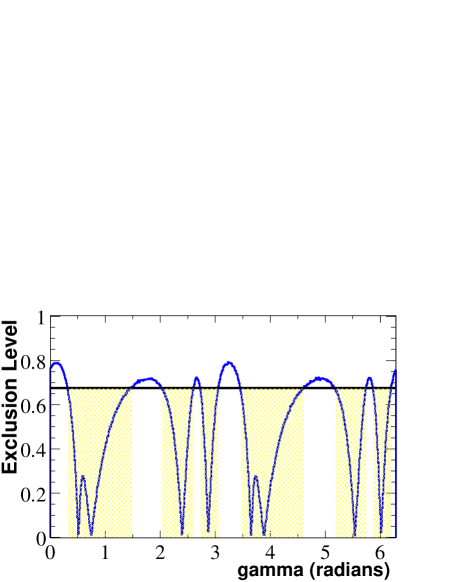
Figure 1: The measured exclusion level, as a function of $\gamma$, from a fit to the vector-vector modes ($D^{*+}D^{*-}$ and $D_{s}^{*+}D^{*-}$). The exclusion level is defined in the text. From the fit, $\gamma$ is favored to lie in one of the ranges $[0.31-1.50](+0\mbox{ or }\pi)$, $[2.02-2.62](+0\mbox{ or }\pi)$, or $[2.72-3.05](+0\mbox{ or }\pi)$ radians at 68% confidence level.

We use a toy Monte Carlo (MC) method to determine the confidence intervals for $\gamma$. We consider 500 values for $\gamma$, evenly spaced between 0 and $2\pi$. For each value of $\gamma$ considered, we generate 25000 toy MC experiments, with inputs that span the range of the experimental errors of each quantity. For each experiment, we generate random values of each of the experimental inputs according to Gaussian distributions, with means and sigmas according to the measured central value and total errors on each experimental quantity. We make the assumption that the ratio $f_{D_{s}^{*}}/f_{D^{*}}$ is equal to $f_{D_{s}}/f_{D}=1.20\pm 0.06\pm 0.06$ [5]. An additional theory error of 10% is included to take into account the assumptions of Eq. (14), as well as smaller errors such as the neglect of the exchange diagram, subdominant SU(3)-breaking terms, etc. We then calculate the resulting values of ${\cal A}_{ct}$, $a_{\rm dir}$, $a_{\rm indir}$, and $B$, given the generated random values (based on the experimental values). Inputting the quantities $a_{\rm dir}$, $a_{\rm indir}$, and $B$, along with $\beta$ and the value of $\gamma$ that is being considered, into Eq. (6), we obtain a residual value for each experiment, equal to the difference of the left- and right-hand sides of the equation. One thus obtains an ensemble of residual values from the 25000 experiments. A likelihood, as a function of $\gamma$, can be obtained from $\chi^{2}(\gamma)$, where $\chi^{2}\equiv(\mu/\sigma)^{2}$, in which $\mu$ is the mean of the above ensemble of residual values and $\sigma$ is the usual square root of the variance. The value of $\chi(\gamma)$ is then considered to represent a likelihood which is equal to that of a value $\chi$ standard devations of a Gaussian distribution from the most likely value(s) of $\gamma$. We define the “exclusion level,” as a function of the value of $\gamma$, as follows: the value of $\gamma$ is excluded from a range at a given C.L. if the exclusion level in that range of $\gamma$ values is greater than the given C.L.

Fig. 1 shows the resulting measured confidence as a function of $\gamma$. We see that $\gamma$ is favored to lie in one of the ranges $[0.31-1.50](+0\mbox{ or }\pi)$, $[2.02-2.62](+0\mbox{ or }\pi)$, or $[2.72-3.05](+0\mbox{ or }\pi)$ radians at 68% C.L. This corresponds to $[18.0^{\circ}-85.7^{\circ}](+0^{\circ}\mbox{ or }$ $180^{\circ})$, $[116^{\circ}-150^{\circ}](+0^{\circ}\mbox{ or }180^{\circ})$, or $[156^{\circ}-175^{\circ}](+0^{\circ}\mbox{ or }180^{\circ})$. Fig. 2 shows a check on the confidence distribution to ensure that it accurately describes the level of uncertainty on the measured value of $\gamma$.

Figure 2: A “pull distribution” check on the measured confidence levels for the $\gamma$ fit. Values of $\gamma$, as well as the other theoretical parameters $\mathcal{A}_{ct}$, $\mathcal{A}_{ut}$, $\delta$, and $\beta$, are generated and used to produce values of the experimental inputs to the fit. The fit is then performed, and ((measured value of $\gamma$) $-$ (generated value of $\gamma$))/(measured uncertainty on $\gamma$) is plotted. The result is consistent with a Gaussian distribution with $\sigma=1$, implying that uncertainty on the measured value of $\gamma$ is accurately described by the confidence distribution.

We now turn to the VP decays $B_{d}^{0}(t)\rightarrow D^{*\pm}D^{\mp}$, $B_{d}^{0}\rightarrow D_{s}^{*+}D^{-}$, and $B_{d}^{0}\rightarrow D_{s}^{+}D^{*-}$. The advantage of the VP method is that no additional assumptions of the type described in Eq. (14) are needed. The disadvantage is that, as we will see, the data are such that no information on the most likely regions of $\gamma$ can be obtained from the VP modes.

In order to implement the VP method, we proceed as follows. We first use the expressions for $B$, $a_{dir}$, ${\tilde{B}}$ and ${\tilde{a}}_{dir}$ in Eqs. (S0.Ex9) and (S0.Ex12) to analytically solve for the theoretical unknowns ${\cal A}_{ut}$, $\tilde{{\cal A}}_{ut}$, $\delta$, and $\delta^{\prime}$, up to a four-fold ambiguity. We then have the two remaining equations for $a_{indir}$ and ${\tilde{a}}_{indir}$ and two theoretical unknowns, $\gamma$ and $\Delta$. We now consider 200 values for each of $\gamma$ and $\Delta$, each evenly spaced between 0 and $2\pi$. For each of the $200\times 200$ possible combinations of values of $\gamma$ and $\Delta$, we generate 5000 toy MC experiments, with inputs that span the range of the experimental errors of each quantity.

Similar to the toy Monte Carlo $\gamma$ determination for the VV mode, we generate random values of each of the experimental inputs according to Gaussian distributions, with means and sigmas according to the measured central value and total errors on each experimental quantity. Making the assumption that $f_{D_{s}^{*}}/f_{D^{*}}$ is equal to $f_{D_{s}}/f_{D}=1.20\pm 0.06\pm 0.06$ [5], we again obtain a confidence distribution as a function of $\gamma$. The result is shown in Fig. 3. As can been seen in this figure, present data on VP decays alone do not lead to useful constraints on $\gamma$.

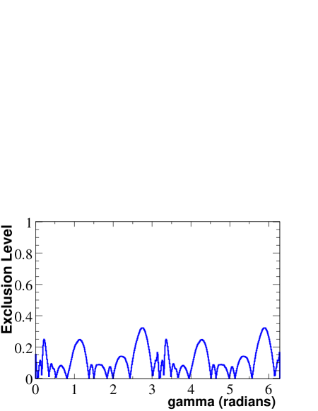
Figure 3: The measured exclusion level, as a function of $\gamma$, from a fit to the vector-pseudoscalar modes $D^{*\pm}D^{\mp}$, $D_{s}^{*+}D^{-}$, and $D_{s}^{+}D^{*-}$. Unlike the vector-vector modes, with present data we do not obtain useful information on the likely regions of $\gamma$ from these modes alone.

Finally, we can combine information from the VV and VP modes. The result is shown in Fig. 4. From the combined fit, we see that $\gamma$ is favored to lie in one of the ranges $[0.34-1.41](+0\mbox{ or }\pi)$, $[2.09-2.57](+0\mbox{ or }\pi)$, or $[2.79-3.04](+0\mbox{ or }\pi)$ radians at 68% confidence level. This corresponds to $[19.4^{\circ}-80.6^{\circ}](+0^{\circ}\mbox{ or }180^{\circ})$, $[120^{\circ}-147^{\circ}](+0^{\circ}\mbox{ or }180^{\circ})$, or $[160^{\circ}-174^{\circ}](+0^{\circ}\mbox{ or }180^{\circ})$. Comparing Figs. 1 and 4, we see that the favored ranges of $\gamma$ are slightly more constrained with the VP data. Thus, although the VP data does not by itself constrain $\gamma$, its inclusion in the combined fit does have an effect.

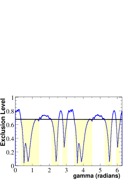
Figure 4: The measured exclusion level, as a function of $\gamma$, from the combined information from vector-vector and vector-pseudoscalar modes. The combined information implies that $\gamma$ is favored to lie in one of the ranges $[0.34-1.41](+0\mbox{ or }\pi)$, $[2.09-2.57](+0\mbox{ or }\pi)$, or $[2.79-3.04](+0\mbox{ or }\pi)$ radians at 68% confidence level.

To summarize, we have presented the extraction of $\gamma$ using measurements of $B_{d}^{0}(t)\rightarrow D^{(*)+}D^{(*)-}$ and $B_{d}^{0}\rightarrow D_{s}^{(*)+}D^{(*)-}$ decays [1]. We find that $\gamma$ is favored to lie in one of the ranges $[19.4^{\circ}-80.6^{\circ}](+0^{\circ}\mbox{ or }180^{\circ})$, $[120^{\circ}-147^{\circ}](+0^{\circ}\mbox{ or }180^{\circ})$, or $[160^{\circ}-174^{\circ}](+0^{\circ}\mbox{ or }180^{\circ})$ at 68% confidence level (the $(+0^{\circ}\mbox{ or }180^{\circ})$ represents an additional ambiguity for each range). The first of these ranges is that favored by fits to the Unitarity Triangle, assuming the standard model. The ranges come principally from data on vector-vector decays, although the vector-pseudoscalar decays do improve the constraints slightly. Note that, if we consider a larger confidence level, there are no constraints on $\gamma$ at present. However, this study demonstrates the feasibility of the method – with more data, we will be able to obtain strong constraints on $\gamma$.

Acknowledgements: We thank Andreas Kronfeld for helpful communications regarding the lattice values of $f_{D_{s}}/f_{D}$ and $f_{D_{s}^{*}}/f_{D^{*}}$. J.A. is partially supported by DOE contract DE-FG01-04ER04-02. The work of A.D. and D.L. is financially supported by NSERC of Canada.

References

• [1] A. Datta and D. London, Phys. Lett. B 584, 81 (2004).
• [2] M. Gronau, O.F. Hernández, D. London and J.L. Rosner, Phys. Rev. D 50, 4529 (1994), Phys. Rev. D 52, 6356 (1995), Phys. Rev. D 52, 6374 (1995).
• [3] Heavy Flavor Averaging Group, world charmonium avg. (Winter 2004), http://www.slac.stanford.edu/xorg/hfag/triangle/winter2004/index.shtml.
• [4] This is always the case when one attempts to obtain weak phase information from a decay involving a ${\bar{b}}\rightarrow{\bar{d}}$ penguin, see D. London, N. Sinha and R. Sinha, Phys. Rev. D 60, 074020 (1999).
• [5] J. Simone, invited talk at Lattice 2004, Fermilab, June 2004:
http://lqcd.fnal.gov/lattice04/presentations/paper252.pdf
• [6] A similar method is described in A. Datta and D. London, Phys. Lett. B 533, 65 (2002). However, there is a mistake in that method, due to the fact that the hadronization is different for the decays $B_{d}^{0}(t)\rightarrow K^{*}{\bar{K}}$ and $B_{d}^{0}(t)\rightarrow K{\bar{K}}^{*}$.
• [7] BaBar Collaboration, B. Aubert et al., Phys. Rev. Lett. 89, 061801 (2002).
• [8] Belle Collaboration, K. Abe et al., Phys. Rev. Lett. 89, 122001 (2002).
• [9] BaBar Collaboration, B. Aubert et al., Phys. Rev. Lett. 90, 221801 (2003).
• [10] Belle Collaboration, K. Abe et al., hep-ph/0408051, submitted to ICHEP 2004, Beijing, August 2004.
• [11] BaBar Collaboration, B. Aubert et al., Phys. Rev. Lett. 91, 131801 (2003).
• [12] CLEO Collaboration, D. Gibaut et al., Phys. Rev. D 53, 4734 (1996).
• [13] BaBar Collaboration, B. Aubert et al., Phys. Rev. D 67, 092003 (Rap. Comm.) (2003).
• [14] A. Höcker et al., Eur. Phys. J. C 21, 225 (2001).
• [15] M. Bona et al., hep-ph/0408079, submitted to ICHEP 2004, Beijing, August 2004.
• [16] G.P. Dubois-Felsmann et al., hep-ph/0308262, submitted to Lepton-Photon 2003, Fermilab, August 2003.
• [17] J.L. Rosner, Phys. Rev. D42, 3732 (1990); Z. Luo and J.L. Rosner, Phys. Rev. D64, 094001 (2001). See also A. Abd El-Hady, A. Datta and J.P. Vary, Phys. Rev. D58, 014007 (1998); A. Abd El-Hady, A. Datta, K.S. Gupta and J.P. Vary, Phys. Rev. D55, 6780 (1997).
• [18] S. Eidelman et al., Phys. Lett. B 592, 1 (2004).