Perturbative QCD Potential and String Tension

The leading non-perturbative contribution to the static QCD potential at $r\ll\Lambda_{\rm QCD}^{-1}$ is known to be ${\cal O}(r^{2})$ in operator-product expansion. It indicates that a “Coulomb+linear” potential at $r\hbox{ \raise 3.0pt\hbox to0.0pt{$<$}\raise-3.0pt\hbox{$\sim$} }\Lambda_{\rm QCD}^{-1}$ is included in the perturbative QCD prediction of the potential. It was shown that this is indeed the case, and the “Coulomb+linear” potential has been systematically computed up to next-to-next-to-leading logarithmic order, in terms of the Lambda parameter in the $\overline{\rm MS}$ scheme ($\Lambda_{\overline{\rm MS}}$). We review the present status of the perturbative prediction for the QCD potential, which takes into account the theoretical breakthrough that took place around 1998.

1 Introduction

In this article we review the present status of perturbative QCD predictions for the QCD potential, in the distance region relevant to the bottomonium and charmonium states, $0.5~{}{\rm GeV}^{-1}(0.1~{}{\rm fm})\hbox{ \raise 3.0pt\hbox to0.0pt{$<$}\raise-3.0pt\hbox{$\sim$} }r\hbox{ \raise 3.0pt\hbox to0.0pt{$<$}\raise-3.0pt\hbox{$\sim$} }5~{}{\rm GeV}^{-1}(1~{}{\rm fm})$. We take into account the theoretical breakthrough that took place around 1998 [1], which improved the accuracy of perturbative prediction dramatically.

For a quite long time, the perturbative QCD predictions of the QCD potential $V_{\rm QCD}(r)$ were not successful in the above distance region. In fact, the perturbative series turned out to be very poorly convergent at $r\hbox{ \raise 3.0pt\hbox to0.0pt{$>$}\raise-3.0pt\hbox{$\sim$} }0.5~{}{\rm GeV}^{-1}$; uncertainty of the series is so large that one could hardly obtain meaningful predictions. Even if one tries to improve the perturbation series by certain resummation prescription (such as renormalization group improvement), scheme dependence of the result was also very large [2]; hence, one could neither obtain accurate prediction of the potential in this distance region. It was later pointed out that the large uncertainty of the perturbative QCD prediction can be understood as caused by the leading-order [${\cal O}(\Lambda_{\rm QCD})$] infrared (IR) renormalon contained in $V_{\rm QCD}(r)$ [3].

On the other hand, empirically it has been known that phenomenological potentials and lattice computations of $V_{\rm QCD}(r)$ are both approximated well by the sum of a Coulomb potential and a linear potential in the above range $0.5~{}{\rm GeV}^{-1}\hbox{ \raise 3.0pt\hbox to0.0pt{$<$}\raise-3.0pt\hbox{$\sim$} }r\hbox{ \raise 3.0pt\hbox to0.0pt{$<$}\raise-3.0pt\hbox{$\sim$} }5~{}{\rm GeV}^{-1}$. (See e.g. [4]). The linear behavior of $V_{\rm QCD}(r)$ at large distances $r\gg\Lambda_{\rm QCD}^{-1}$ (verified numerically by lattice computations) is consistent with the quark confinement picture. For this reason, and given the very poor predictability of perturbative QCD, it was often said that, while the “Coulomb” part of $V_{\rm QCD}(r)$ (with logarithmic correction at short-distances) is contained in the perturbative QCD prediction, the linear part is purely non-perturbative and absent in the perturbative QCD prediction even at $r\hbox{ \raise 3.0pt\hbox to0.0pt{$<$}\raise-3.0pt\hbox{$\sim$} }\Lambda_{\rm QCD}^{-1}$, and that the linear potential needs to be added to the perturbative prediciton to obtain the full QCD potential. See Fig. 1.

\psfrag{r}{\raise 1.0pt\hbox{$r~{}~{}[{\rm GeV}^{-1}]$}}\psfrag{Potential}{ Potential~{}~{}~{}~{}[GeV]}\psfrag{Coulomb Pot.}{Coulomb Pot.}\psfrag{Phenomenological Pot.}{\color[rgb]{0,0,1}{Phenomenological Pot.}}\psfrag{breakdown}{\color[rgb]{.8,0,0}{\small breakdown of pert.\ prediction}}\includegraphics[width=213.39566pt]{Vc-Vpheno4.eps}

Figure 1: Status of theoretical predictions for the QCD potential before the discovery of renormalon cancellation. One could hardly see sign of convergence of perturbative series at $r\hbox{ \raise 3.0pt\hbox to0.0pt{$>$}\raise-3.0pt\hbox{$\sim$} }0.5~{}{\rm GeV}^{-1}$.

Nevertheless, to the best of our knowledge, there was no firm theoretical basis for this argument.

Several years ago, the perturbative prediction of the QCD potential became much more accurate in this region. There were two important developments: (1) The complete ${\cal O}(\alpha_{S}^{3})$ corrections to the QCD potential have been computed [5]; also the relation between the quark pole mass and the $\overline{\rm MS}$ mass has been computed up to ${\cal O}(\alpha_{S}^{3})$ [6]. (2) A renormalon cancellation was discovered [1] in the total energy of a static $Q\bar{Q}$ pair, $E_{\rm tot}(r)\equiv 2m_{\rm pole}+V_{\rm QCD}(r)$. Consequently, convergence of the perturbative series of $E_{\rm tot}(r)$ improves drastically, if it is expressed in terms of the quark $\overline{\rm MS}$ mass instead of the pole mass.

Physically, improvement of convergence stems from decoupling of IR gluons from the color-singlet $Q\bar{Q}$ system. Intuitively, IR gluons, whose wavelengths are larger than $r$, cannot see the color charge of $Q$ or $\bar{Q}$ but only see the total charge of this system. Therefore, in the computation of the total energy of the $Q\bar{Q}$ system, we expect that contributions of IR gluons should decouple. This is naturally realized, if we use a quark mass, which is renormalized to include contributions of only UV gluons, such as the $\overline{\rm MS}$ mass; in this case, there is a cancellation of IR contributions between the self-energies of $Q/\bar{Q}$ and the potential energy. If we use a mass, which includes also contributions of IR gluons, such as the pole mass, then the decoupling of IR gluons is not realized. Generally, convergence of a perturbative expansion is worse when there are more contributions from IR gluons, and vice versa.

Let us demonstrate the improvement of accuracy of the perturbative prediction for the total energy $E_{\rm tot}(r)$ up to ${\cal O}(\alpha_{S}^{3})$, when the cancellation of ${\cal O}(\Lambda_{\rm QCD})$ renormalons is incorporated. As an example, we take the bottomonium case: We choose the $\overline{\rm MS}$ mass of the $b$-quark, renormalized at the $b$-quark $\overline{\rm MS}$ mass, as $\overline{m}_{b}\equiv m_{b}^{\overline{\rm MS}}(m_{b}^{\overline{\rm MS}})=4.190$ GeV; in internal loops, four flavors of light quarks are included with $\overline{m}_{u}=\overline{m}_{d}=\overline{m}_{s}=0$ and $\overline{m}_{c}=1.243$ GeV. (See the formula for $E_{{\rm tot}}^{b\bar{b}}(r)$ in [7].) In Fig. 2, we fix $r=2.5~{}{\rm GeV}^{-1}$ (midst in the distance range of our interest) and examine the renormalization-scale ($\mu$) dependences of $E_{{\rm tot}}(r)$.

\psfrag{mu}{$\mu$~{}[GeV]}\psfrag{Etot}{\hskip 5.69054pt$E_{\rm tot}(r)$~{}~{}[GeV]}\psfrag{r = 2.5}{$r=2.5$~{}GeV${}^{-1}$}\psfrag{Pole-mass scheme}{\raise 0.0pt\hbox{Pole-mass scheme}}\psfrag{MSbar-mass scheme}{$\overline{\rm MS}$-mass scheme}\includegraphics[width=170.71652pt]{mu-dep.eps}

Figure 2: Scale dependences of $E_{{\rm tot}}^{b\bar{b}}(r)$ up to ${\cal O}(\alpha_{S}^{3})$ at $r=2.5~{}{\rm GeV}^{-1}$, in the pole-mass and $\overline{\rm MS}$-mass schemes. A horizontal line at $8$ GeV is plotted as a guide.

We see that $E_{{\rm tot}}(r)$ is much less scale dependent when we use the $\overline{\rm MS}$ mass than when we use the pole mass. Hence, the perturbative prediction of $E_{{\rm tot}}(r)$ is much more stable in the former scheme.

We also compare the convergence behaviors of the perturbative series of $E_{\rm tot}$ for the same $r$ and when $\mu$ is fixed to the value, at which $E_{\rm tot}$ becomes least sensitive to variation of $\mu$ (minimal-sensitivity scale). Convergence of the perturbation series turns out to be close to optimal for this scale choice: at $r=2.5~{}{\rm GeV}^{-1}$, the minimal-sensitivity scale is $\mu=0.90$ GeV. We find

$$E_{{\rm tot}}^{b\bar{b}}(r) = 10.408-0.275-0.362-0.784~{}~{}{\rm GeV}~{}~{}\mbox{(Pole-mass scheme)}$$ (1)

$$= ~{}\,8.380+1.560-0.116-0.022~{}~{}{\rm GeV}~{}~{}\mbox{($\overline{\rm MS}$-mass scheme)}.$$ (2)

The four numbers represent the ${\cal O}(\alpha_{S}^{0})$, ${\cal O}(\alpha_{S}^{1})$, ${\cal O}(\alpha_{S}^{2})$ and ${\cal O}(\alpha_{S}^{3})$ terms of the series expansion in each scheme. The ${\cal O}(\alpha_{S}^{0})$ terms represent merely the twice of the pole mass and of the $\overline{\rm MS}$ mass, respectively. As can be seen, if we use the pole mass, the series is not converging beyond ${\cal O}(\alpha_{S}^{1})$. On the other hand, in the $\overline{\rm MS}$-mass scheme, the series is converging. One may also verify that, when the series is converging ($\overline{\rm MS}$-mass scheme), $\mu$-dependence of $E_{\rm tot}(r)$ decreases as we include more terms of the perturbative series, whereas when the series is diverging (pole-mass scheme), $\mu$-dependence does not decrease with increasing order. (See e.g. [8].)

We observe qualitatively the same features at different $r$ and for different number of light quark flavors $n_{l}$, or when we change values of the masses $\overline{m}_{b}$, $\overline{m}_{c}$. Generally, at smaller $r$, $E_{\rm tot}(r)$ becomes less $\mu$-dependent and more convergent, due to asymptotic freedom. See [7, 9] for details.

The aim of this paper is to review the properties of $E_{\rm tot}(r)$, given the much more accurate prediction as compared to several years ago. In Sec. 2 we examine $E_{\rm tot}(r)$ up to ${\cal O}(\alpha_{S}^{3})$. Sec. 3 provides a classification of perturbative and non-perturbative contributions to $E_{\rm tot}(r)$ in terms of operator-product-expansion (OPE). We present our main result, that the perturbative prediction of the leading short-distance contribution to $E_{\rm tot}(r)$ is given as a “Coulomb+linear” potential, in Sec. 4. Conclusions are given in Sec. 5.

2 Pert. prediction of $E_{\rm tot}(r)$ up to ${\cal O}(\alpha_{S}^{3})$

Let us first review comparisons of the perturbative predictions of $E_{\rm tot}(r)$ up to ${\cal O}(\alpha_{S}^{3})$ with phenomenological potentials and with lattice computations of the QCD potential.

In Fig. 3, $E_{\rm tot}(r)$ is compared with typical phenomenological potentials.

\psfrag{XXX}{\footnotesize$r~{}[{\rm GeV}^{-1}]$}\psfrag{YYY}{\footnotesize Energy~{}~{}~{}$[{\rm GeV}]$}\psfrag{PowerLaw}{\footnotesize Power--law potential}\psfrag{Log}{\footnotesize Log potential}\psfrag{Cornell}{\footnotesize Cornell potential}\psfrag{1161}{\footnotesize$\alpha_{s}(M_{Z})=0.1161$}\psfrag{1181}{\footnotesize$\alpha_{s}(M_{Z})=0.1181$}\psfrag{1201}{\footnotesize$\alpha_{s}(M_{Z})=0.1201$}\psfrag{u1s}{\footnotesize$\Upsilon(1S)$}\psfrag{u2s}{\footnotesize$\Upsilon(2S)$}\psfrag{u3s}{\footnotesize$\Upsilon(3S)$}\psfrag{u4s}{\footnotesize$\Upsilon(4S)$}\psfrag{j1s}{\footnotesize$J/\psi$}\psfrag{j2s}{\footnotesize$\psi(2S)$}\includegraphics[width=256.0748pt]{figpot.eps}

Figure 3: $E_{\rm tot}(r)$ and typical phenomenological potentials. Constants are added to make all curves coincide at $r=1~{}{\rm GeV}^{-1}$. Arrows at the bottom show the r.m.s. radii of the heavy quarkonium states. The figure is taken from [7].

Since the latter are determined from the heavy quarkonium spectra, realistic values for the input parameters of $E_{\rm tot}(r)$, as given in the previous section, have been chosen. The scale $\mu=\mu(r)$ is fixed by either $\partial E_{\rm tot}/\partial\mu=0$ (minimum sensitivity scale) or $|E_{\rm tot}^{(3)}|=\mbox{minimum}$, but both prescriptions lead to almost same values of $E_{\rm tot}(r)$. See [10, 7, 9] for details. We see that $E_{\rm tot}(r)$ corresponding to the present values of the strong coupling constant (dashed lines) agree well with the phenomenological potentials within estimated perturbative uncertainties (indicated by error bars). We also note that the agreement is lost quickly if we take $\alpha_{S}(M_{Z})$ outside of the present world-average values, so that the agreement is unlikely to be accidental.

In fact, by now several works have confirmed agreements of the perturbative predictions of the QCD potential with phenomenological potentials or with lattice computations [10, 11, 7, 12, 13, 9]. Although details depend on how the renormalon in the QCD potential is cancelled, qualitatively the same conclusions were drawn: i.e. perturbative predictions become accurate and agree with phenomenological potentials/lattice results up to much larger $r$ than before. In particular, in the differences between the perturbative predictions and phenomenological potentials/lattice results, a linear potential of order $\Lambda_{\rm QCD}^{2}r$ at distances $r\hbox{ \raise 3.0pt\hbox to0.0pt{$<$}\raise-3.0pt\hbox{$\sim$} }\Lambda_{\rm QCD}^{-1}$ was ruled out numerically. In other words, one cannot get the full QCD potential if one adds a linear potential to the perturbative QCD potential (after renormalon cancellation).

A crucial point is that, once the ${\cal O}(\Lambda_{\rm QCD})$ renormalon is cancelled and the perturbative prediction is made accurate, the perturbative potential becomes steeper than the Coulomb potential as $r$ increases. This feature is understood, within perturbative QCD, as an effect of the running of the strong coupling constant [14, 10, 11]. In short, the interquark force becomes stronger than the Coulomb force at larger $r$ by this effect.

3 Operator-product expansion of $V_{\rm QCD}(r)$

Operator-product expansion (OPE) of $V_{\rm QCD}(r)$ for $r\ll\Lambda_{\rm QCD}^{-1}$ was developed [15] within an effective field theory “potential non-relativistic QCD” (pNRQCD) [16]. In this framework, $V_{\rm QCD}(r)$ is expanded in $r$ (multipole expansion), when the following hierarchy of scales exists:

$$\Lambda_{\rm QCD}\ll\mu_{f}\ll\frac{1}{r}.$$ (3)

Here, $\mu_{f}$ denotes the factorization scale. At each order of the expansion in $r$, short-distance contributions ($q>\mu_{f}$) are factorized into perturbatively computable Wilson coefficients and long-distance contributions ($q<\mu_{f}$) into matrix elements of operators, i.e. non-perturbative quantities. The leading non-perturbative contribution to the potential turns out to be ${\cal O}(\Lambda_{\rm QCD}^{3}r^{2})$.

Explicitly, the QCD potential is given by

$$V_{\rm QCD}(r)=V_{S}(r;\mu_{f})+\delta E_{\rm US}(r;\mu_{f}),$$ (4)

$$\delta E_{\rm US}=-ig_{S}^{2}\frac{T_{F}}{N_{C}}\int_{0}^{\infty}\!\!dt\,e^{-i\,\Delta V(r)\,t}\,\left<{0}\,\right|\vec{r}\!\cdot\!\vec{E}^{a}(t)\,\varphi_{\rm adj}(t,0)^{ab}\,\vec{r}\!\cdot\!\vec{E}^{b}(0)\left|\,{0}\,\right>$$

$$~{}~{}~{}~{}~{}~{}~{}~{}~{}~{}+~{}{\cal O}(r^{3}).$$ (5)

The leading short-distance contribution to $V_{\rm QCD}(r)$ is given by the singlet potential $V_{S}(r)$. It is a Wilson coefficient, which represents the potential between the static $Q\bar{Q}$ pair in color singlet state. The leading non-perturbative contribution [${\cal O}(r^{2})$ in the multipole expansion] is contained in the matrix element in eq. (5). $\Delta V(r)=V_{O}(r)-V_{S}(r)$ denotes the difference between the octet and singlet potentials; see [15] for details.

The singlet potential $V_{S}(r;\mu_{f})$ can be computed in perturbative expansion in $\alpha_{S}$ by matching pNRQCD to QCD. It is essentially the perturbative expansion of $V_{\rm QCD}(r)$ after the contribution of soft degrees of freedom ($q<\mu_{f}$) is subtracted. In particular, the IR divergences and IR renormalons contained in the perturbative expansion of $V_{\rm QCD}(r)$ have been subtracted via appropriate renormalization prescription [15, 12, 18]. Thus, $V_{S}(r;\mu_{f})$ can be computed accurately by perturbative QCD.

We may understand why the leading non-perturbative contribution is ${\cal O}(r^{2})$ as follows. As well known, the leading interaction (in expansion of $r$) between soft gluons and a color-singlet $Q\bar{Q}$ state of size $r$ is given by the dipole interaction $\vec{r}\cdot\vec{E}^{a}$, where $\vec{E}^{a}$ denotes the color electric field. It turns the color singlet $Q\bar{Q}$ state into a color octet $Q\bar{Q}$ state by emission of soft gluon(s). To return to the color singlet $Q\bar{Q}$ state, it needs to reabsorb the soft gluon(s), which requires an additional dipole interaction. Thus, the leading contribution of soft gluons to the total energy is ${\cal O}(r^{2})$.

4 Pert. prediction of $V_{S}(r)$ up to NNLL:
“Coulomb+linear” potential

Here, we present our main result. As already stated, the singlet potential $V_{S}(r;\mu_{f})$ can be computed in perturbative QCD, which may be improved via renormalization group (RG). We have shown that $V_{S}(r;\mu_{f})$ thus computed can be expressed as a “Coulomb+linear” potential, up to an ${\cal O}(r^{2})$ correction. The correction can be absorbed into the ${\cal O}(r^{2})$ non-perturbative contribution $\delta E_{\rm US}(r;\mu_{f})$ by appropriate renormalization prescription. Explicitly, we find [17, 18]

$$V_{S}(r;\mu_{f})={\rm const.}+V_{\rm C}(r)+\sigma\,r+{\cal O}(\mu_{f}^{3}r^{2}),$$ (6)

where

$$V_{\rm C}(r)=-\frac{4\pi C_{F}}{\beta_{0}r}-\frac{2C_{F}}{\pi}\,{\rm Im}\int_{C_{1}}\!dq\,\frac{e^{iqr}}{qr}\,\alpha_{V}(q),$$ (7)

$${\sigma}=\frac{C_{F}}{2\pi i}\int_{C_{2}}\!dq\,q\,\alpha_{V}(q).$$ (8)

In the above equations, $\alpha_{V}(q)$ denotes the perturbative evaluation of the $V$-scheme coupling constant in momentum space [5] (improved by RG, after subtraction of IR divergences via renormalization). The integral paths $C_{1}$ and $C_{2}$ are displayed in Figs. 4.

\psfrag{C1}{$C_{1}$}\psfrag{q}{$q$}\psfrag{q*}{$q_{*}$}\psfrag{0}{\raise-2.84526pt\hbox{$0$}}\includegraphics[width=128.0374pt]{path1.eps}

\psfrag{C2}{$C_{2}$}\psfrag{q}{$q$}\psfrag{q*}{$q_{*}$}\psfrag{0}{\raise-2.84526pt\hbox{$0$}}\includegraphics[width=128.0374pt]{path2.eps}

Figure 4: Integral contours $C_{1}$ and $C_{2}$ on the complex $q$-plane. $q_{*}$ denotes the Landau singularity of $\alpha_{S}(q)$. For 1-loop running, $q_{*}$ is a pole; for 2- and 3-loop running, $q_{*}$ is a branch point. In the latter case, branch cut is on the real axis starting from $q_{*}$ to $-\infty$.

$V_{\rm C}(r)$ and $\sigma$ are defined to be independent of $\mu_{f}$ (at least) up to NNLL. $C_{F}=4/3$ denotes a color factor; $\beta_{0}=11-2n_{l}/3$ represents the 1-loop coefficient of the beta function. In eq. (6), we are not concerned about the constant ($r$-independent) part of $V_{S}(r)$, keeping in mind that it can always be absorbed into $2m_{\rm pole}$ in the total energy $E_{\rm tot}(r)$.

By evaluating the above integral, the coefficient of the linear potential $\sigma$ can be expressed analytically in terms of the Lambda parameter in the $\overline{\rm MS}$-scheme $\Lambda_{\overline{\rm MS}}$. For instance, at LL, it is given by

$$\sigma_{\rm LL}=\frac{2\pi C_{F}}{\beta_{0}}\,\left(\Lambda_{\overline{\rm MS}}^{\rm 1-loop}\right)^{2}.$$ (9)

The “Coulomb” potential has a short-distance asymptotic behavior consistent with RG,

$$V_{\rm C}(r)\sim-\frac{2\pi C_{F}}{\beta_{0}r\ln\Bigl{(}\frac{1}{r\Lambda_{\overline{\rm MS}}}\Bigr{)}}~{}~{}~{}~{}~{}(r\to 0),$$ (10)

whereas its long-distance behavior is given by

$$V_{\rm C}(r)\sim-\frac{4\pi C_{F}}{\beta_{0}r}~{}~{}~{}~{}~{}(r\to\infty).$$ (11)

In the intermediate region both asymptotic forms are smoothly interpolated.

Fig. 5 shows the Coulomb+linear potentials

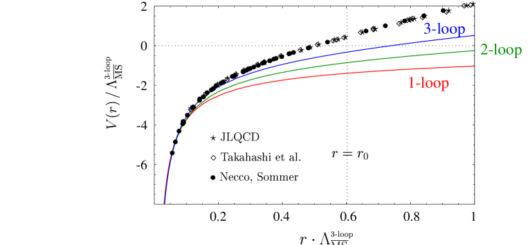
Figure 5: Comparison of the Coulomb+linear potential ($n_{l}=0$) with the lattice results in the quenched approximation. 1-, 2- and 3-loop correspond, respectively, to LL, NLL and NNLL in the RG-improved computation of $V_{S}(r)$.

corresponding to the RG improvement by the 1-loop running (LL), 2-loop running with 1-loop non-logarithmic term (NLL), and 3-loop running with 2-loop non-logarithmic term (NNLL). They are compared with the lattice results. Since the 3-loop non-logarithmic term is not yet known, the 3-loop running case represents our current best knowledge. Up to this order, the Coulomb+linear potential agrees with the lattice results up to larger $r$ as we increase the order.

5 Conclusions

After discovery of renormalon cancellation, perturbative prediction of the total energy $E_{\rm tot}(r)=2m_{\rm pole}+V_{\rm QCD}(r)$ became much more accurate in the distance range $0.5~{}{\rm GeV}^{-1}\hbox{ \raise 3.0pt\hbox to0.0pt{$<$}\raise-3.0pt\hbox{$\sim$} }r\hbox{ \raise 3.0pt\hbox to0.0pt{$<$}\raise-3.0pt\hbox{$\sim$} }5~{}{\rm GeV}^{-1}$. Consequently we observe the following:

• Perturbative prediction of $E_{\rm tot}(r)$ up to ${\cal O}(\alpha_{S}^{3})$ agrees well with phenomenological potentials/lattice results within the estimated perturbative uncertainty.

• According to OPE, the leading non-perturbative contribution to $E_{\rm tot}(r)$ in expansion in $r$ is ${\cal O}(r^{2})$.

• Perturbative QCD prediciton of the singlet potential $V_{S}(r)$ (leading Wilson coefficient in OPE) can be written as a “Coulomb+linear” potential. Up to NNLL, the Coulomb+linear potential shows a converge towards lattice results.

All the theoretical analyses conclude that, there is no freedom to add a linear potential of ${\cal O}(\Lambda_{\rm QCD}^{2}r)$ to the perturbative prediction of the QCD potential at $r\hbox{ \raise 3.0pt\hbox to0.0pt{$<$}\raise-3.0pt\hbox{$\sim$} }\Lambda_{\rm QCD}^{-1}$. Therefore, if we are able to define the string tension from the shape of the potential at $r\hbox{ \raise 3.0pt\hbox to0.0pt{$<$}\raise-3.0pt\hbox{$\sim$} }\Lambda_{\rm QCD}^{-1}$ (it has been empirically the case in phenomenological potential model approach), the string tension may be within the reach of perturbative prediction.

References

- [1] A. Pineda, Ph.D. Thesis; A. Hoang, M. Smith, T. Stelzer and S. Willenbrock, Phys. Rev. D59, 114014 (1999); M. Beneke, Phys. Lett. B434, 115 (1998).
- [2] G. Grunberg, Phys. Rev. D40, 680 (1989).
- [3] U. Aglietti and Z. Ligeti, Phys. Lett. B364, 75 (1995).
- [4] G. Bali, Phys. Rept. 343, 1 (2001).
- [5] M. Peter, Phys. Rev. Lett. 78, 602 (1997); Y. Schröder, Phys. Lett. B447, 321 (1999).
- [6] K. Melnikov and T. v. Ritbergen, Phys. Lett. B482, 99 (2000).
- [7] S. Recksiegel and Y. Sumino, Phys. Rev. D 65, 054018 (2002).
- [8] Y. Kiyo and Y. Sumino, Phys. Rev. D67, 071501 (2003) (Rapid Comm.).
- [9] S. Recksiegel and Y. Sumino, Eur. Phys. J. C 31, 187 (2003).
- [10] Y. Sumino, Phys. Rev. D 65, 054003 (2002).
- [11] S. Necco and R. Sommer, Phys. Lett. B 523, 135 (2001);
- [12] A. Pineda, J. Phys. G 29, 371 (2003);
- [13] T. Lee, Phys. Rev. D 67, 014020 (2003).
- [14] N. Brambilla, Y. Sumino and A. Vairo, Phys. Lett. B 513, 381 (2001).
- [15] N. Brambilla, A. Pineda, J. Soto and A. Vairo, Phys. Rev. D 60, 091502 (1999); Nucl. Phys. B 566, 275 (2000).
- [16] A. Pineda and J. Soto, Nucl. Phys. Proc. Suppl. 64, 428 (1998).
- [17] Y. Sumino, Phys. Lett. B 571, 173 (2003).
- [18] Y. Sumino, Phys. Lett. B 595, 387 (2004).
- [19] A. Pineda and J. Soto, Phys. Lett. B495, 323 (2000).