TUM-HEP-554/04

UCSD/PTH 04-13

hep-ph/0409293

September 2004

$\bar{B}\to X_{s}l^{+}l^{-}$ in the MSSM at NNLO

Christoph Bobeth^a,b, Andrzej J. Buras^a and Thorsten Ewerth^a

^a Physik Department, Technische Universität München, D-85748 Garching, Germany
^b Physics Department, University of California at San Diego, La Jolla, CA 92093, USA

Abstract

We present the results of the calculation of QCD corrections to the matching conditions for the Wilson coefficients of operators mediating the transition $b\to sl^{+}l^{-}$ in the context of the MSSM. Within a scenario with decoupled heavy gluino the calculated contributions together with those present already in the literature allow for the first time a complete NNLO analysis of $\bar{B}\to X_{s}l^{+}l^{-}$. We study the impact of the QCD corrections and the reduction of renormalization scale dependencies for the dilepton invariant mass distribution and the forward-backward asymmetry in the inclusive decay $\bar{B}\to X_{s}l^{+}l^{-}$ restricting the analysis to the “low-$s$” region and small values of $\tan\beta$. The NNLO calculation allows to decrease the theoretical uncertainties related to the renormalization scale dependence below the size of supersymmetric effects in $\bar{B}\to X_{s}l^{+}l^{-}$ depending on their magnitude. While it will be difficult to distinguish the MSSM expectations for the branching ratio from the Standard Model ones, this can become possible in the dilepton invariant mass distribution depending on the MSSM parameters and $\hat{s}$. In this respect the position of the zero of the forward-backward asymmetry $\hat{s}_{0}$ is even more promising.

                                           
*E-mail addresses: bobeth@su3.ucsd.edu, aburas@ph.tum.de, tewerth@ph.tum.de

1 Introduction

The recent measurements of the branching ratio of the inclusive decay $\bar{B}\to X_{s}l^{+}l^{-}$ ($l=e,\,\mu$) of the Belle Collaboration [2] and the BaBar Collaboration [3] are expected to provide an important test of the Standard Model (SM) and possible new physics effects at the electroweak scale. Furthermore they allow for the extraction of informations complementary to those from the radiative inclusive decay mode $\bar{B}\to X_{s}\gamma$ which is nowadays well known both experimentally and theoretically in the SM and puts non-trivial constraints on parameters of models beyond the SM.

In the discussion of the decay $\bar{B}\to X_{s}l^{+}l^{-}$ the major theoretical uncertainties arise from the non-perturbative nature of intermediate $c\bar{c}$ states of the decay chain $\bar{B}\to X_{s}J/\psi\to X_{s}l^{+}l^{-}$ and analogous higher resonances. These decay channels interfere with the simple flavour changing decay mechanism $\bar{B}\to X_{s}l^{+}l^{-}$ and the dilepton invariant mass distribution can be only roughly estimated when the invariant mass of the lepton pair $s\equiv q^{2}=(p_{l^{-}}+p_{l^{+}})^{2}$ is not significantly away from $M_{J/\psi}^{2}$ resulting in uncertainties larger than $\pm 20\%$ [4]. For this reason the charmonium decays are vetoed explicitly in the experimental analysis [2, 3] by cuts on the invariant dilepton mass around the masses of the $J/\psi$ and $\psi^{\prime}$ resonances.

A rather precise determination of the dilepton invariant mass spectrum seems to be possible once the values of $s$ are restricted to be below or above these resonances. Then the calculation can be performed using perturbative methods whereas non-perturbative corrections can be addressed within the framework of Heavy Quark Expansion (HQE). However, contrary to the semileptonic decay $\bar{B}\to X_{u,c}l\bar{\nu}_{l}$ and the radiative decay $\bar{B}\to X_{s}\gamma$ this method is not applicable in the endpoint region of the spectrum as pointed out in [5]. Here other approaches have to be used such as for example Heavy Hadron Chiral Perturbation Theory (HH$\chi$PT) by summing over the kinematically allowed exclusive channels to reliably estimate the magnitude of the endpoint decay spectrum.

At the moment the low-$s$ region, accessible to $l=e$ and $\mu$, is theoretically best understood. The non-perturbative corrections $(\Lambda_{\rm QCD}/m_{b})^{n}$ to the dilepton invariant mass distribution are calculated up to the order $n=3$ [6, 7, 8, 5, 9] and turn out to be small compared to the leading perturbative contribution – however, still involving poorly known matrix elements of the Heavy Quark Effective Theory (HQET) for $n=3$. Furthermore the effects related to the tails of $c\bar{c}$ resonances in the low-$s$ region of the decay $\bar{B}\to X_{s}l^{+}l^{-}$ were estimated model-independently by employing an expansion in inverse powers of the charm quark mass in [10] and the size of these $\Lambda_{\rm QCD}^{2}/m_{c}^{2}$ corrections was found to be similar to the size of $\Lambda_{\rm QCD}^{2}/m_{b}^{2}$ corrections. Because of the smallness of the non-perturbative corrections in the low-$s$ region, the $\bar{B}\to X_{s}l^{+}l^{-}$ decay rate is precisely predictable up to about $10\%$ uncertainty.

The calculations of the perturbative contribution [11, 12, 13] up to the complete next-to-leading order (NLO) in QCD [14, 15] in the SM had not reached this precision. In a series of recent papers the calculation was extended to the next-to-next-to leading order (NNLO) in QCD being almost complete up to the missing two-loop matrix element contributions of the four quark operators $\mathcal{O}_{3}$–$\mathcal{O}_{6}$ which are expected to be small. These calculations comprise

• corrections to the Wilson coefficients [18],

• the anomalous dimension matrices (ADM) of the renormalization group evolution of the Wilson coefficients [19, 20, 21, 22]

• the virtual and real corrections to the matrix elements of the relevant operators [23, 24, 25].

Within the SM the inclusion of NNLO corrections reduces the branching ratios of $\bar{B}\to X_{s}e^{+}e^{-}$ and $\bar{B}\to X_{s}\mu^{+}\mu^{-}$ by typically $12\%$ and $20\%$, respectively [26]. Furthermore uncertainties due to the dependence on the renormalization scale of the top quark mass $\mu_{t}\sim M_{W}$ become reduced from about $\pm 16\%$ to $3\%$ [18] and the inclusion of the NNLO matrix element corrections decrease the low energy scale dependence $\mu_{b}\sim m_{b}$ from $\pm 13\%$ to a value about $\pm 6.5\%$ [23, 24]. Furthermore electroweak corrections were found to be a few percent [22] removing the scale ambiguity of $\alpha_{e}$ when going beyond LO.

Apart from the branching ratio and the dilepton invariant mass distribution, the differential forward-backward asymmetry of leptons represents the third interesting observable in the decay $\bar{B}\to X_{s}l^{+}l^{-}$. The leading contribution to the forward-backward asymmetry arises in the SM at the NLO and thus the inclusion of the NNLO corrections drastically reduces the renormalization scale dependence in predictions of this observable. In particular it is very sensitive to new physics effects and further, $\hat{s}_{0}=s_{0}/m_{b}^{2}$, the position at which the forward-backward asymmetry vanishes provides an important test of the SM [27]. Within the SM the inclusion of NNLO corrections in the evaluation of $\hat{s}_{0}$ leads to a shift of $10\%$ to higher values accompanied by a reduction of the uncertainty due to renormalization scale dependencies in the prediction from typically $15\%$ to $5\%$ [28, 29, 30]. The electroweak corrections shift $\hat{s}_{0}$ by $+2\%$ [22].

Clearly, in view of the improving experimental situation of the ongoing $B$-physics dedicated experiments, such as the BaBar and Belle experiments, hopefully the experimental uncertainties will decrease. Presently it is desirable from the theoretical side to restrict future experimental analysis of the dilepton invariant mass distribution to regions below and above the $c\bar{c}$-resonances.

Besides testing the SM, once the experimental accuracy improves, the inclusive decay $\bar{B}\to X_{s}l^{+}l^{-}$ will also allow to constraint models involving new physics scenarios beyond the SM. The reliability of such constraints depend crucially on theoretical uncertainties due to higher order corrections in the prediction of observables as demonstrated by the SM analysis in the case of the importance of NNLO QCD corrections. In the present work we report the results of a calculation of QCD corrections to the matching conditions for the Wilson coefficients of operators mediating the transition $b\to sl^{+}l^{-}$ in the context of the Minimal Supersymmetric Standard Model (MSSM). We chose a scenario in which the down-squark mass matrix decomposes into $2\times 2$ matrices for each generation and furthermore a heavy decoupled gluino within the MSSM parameter space ensuring the completeness of the calculated QCD corrections.

The scenario of the MSSM that we study here has been introduced in [31] as “Scenario B” (see also [32]). It is a generalization of the “Scenario A” which was used in the context of the calculation of the QCD corrections to $\bar{B}\to X_{s,d}\nu\bar{\nu}$, $\bar{B}_{s,d}\to l^{+}l^{-}$, $K\to\pi\nu\bar{\nu}$ and $K_{L}\to\mu^{+}\mu^{-}$ in the MSSM [33]. In this paper QCD corrections to the relevant $Z^{0}$ penguin diagrams, the box diagrams and the neutral Higgs penguin diagrams have been calculated. While the results of these calculations were ingredients of a NLO analysis of the decays considered there, they contribute to $\bar{B}\to X_{s}l^{+}l^{-}$ first at the NNLO level and consequently enter our present analysis. Actually as we concentrate on the region $\tan\beta\leq 10$, only $Z^{0}$ penguin diagrams and box diagrams calculated in [33] are relevant here. The large $\tan\beta$ region where also neutral Higgs penguins are relevant, will not be considered here.

Taking into account the results of [33], the known results for the Wilson coefficients of the magnetic penguins, the NNLO corrections to the matrix elements of the relevant operators from [23, 24, 25] and their three loop anomalous dimensions calculated recently in [19, 20, 21, 22], the only missing ingredients of a complete NNLO analysis of $\bar{B}\to X_{s}l^{+}l^{-}$ in the MSSM are the QCD corrections to the Wilson coefficients of the four-quark operators $\mathcal{O}_{1}$–$\mathcal{O}_{6}$ and the semileptonic operator $\mathcal{O}_{9}$. These missing ingredients are calculated here for the first time.

The main objectives of our paper are then as follows:

• the calculation of the matching conditions in question at $O(\alpha_{s})$ which requires the evaluation of a large number of two-loop diagrams,

• the calculation of the dilepton invariant mass distribution in $\bar{B}\to X_{s}l^{+}l^{-}$ and of the related forward-backward asymmetry in the MSSM at low $s$ and $\tan\beta$,

• the investigation of the renormalization scale dependence of the observables in question and of the impact of the NNLO corrections on these observables in comparison with the NLO results,

• the comparison of the NNLO results in the MSSM with those obtained in the SM,

• the comparison of the size of MSSM corrections with the theoretical uncertainties in the SM.

The outline of this paper is as follows. In Section 2 we briefly review the elements of the MSSM relevant to the scenario with decoupled gluinos. Section 3 summarizes the low-energy effective Lagrangian for the transition $b\to sl^{+}l^{-}$ and the corresponding Wilson coefficients including $O(\alpha_{s})$ corrections in the context of the MSSM. Section 4 presents the formulae for the dilepton invariant mass distribution and the forward-backward asymmetry of the leptons in the decay $\bar{B}\to X_{s}l^{+}l^{-}$ including all NNLO corrections. The phenomenological implications for both observables will be given in Section 5. We summarize and conclude in Section 6. Finally the appendices collect the analytical results of the Wilson coefficients.

2 The considered Scenario of the MSSM

Let us start by specifying the scenario of the MSSM in which the analytical calculation will be performed. First, we take the down-squark mass-squared matrix to be flavour diagonal so that there are no neutralino contributions to flavour-changing $b\to s$ transitions, and second, we assume the gluino with mass $M_{\tilde{g}}$ to be much heavier than all other sparticles. This first assumption corresponds to “Scenario B” described in detail in [31] which was also used in [32]. The second assumption leads us to an “effective MSSM” with decoupled gluino at the scale $\mu_{\tilde{g}}\sim M_{\tilde{g}}$ [34]. Neglecting all the $1/M_{\tilde{g}}$ effects, the only modified couplings relevant for the NNLO corrections to $\bar{B}\to X_{s}l^{+}l^{-}$ come from the “chargino – up-squark – down-quark” vertex,

$$X_{i}^{U_{L}} =-g_{2}\left[a_{g}\;V_{i1}^{\ast}\;\Gamma^{U_{L}}-a_{Y}\;V_{i2}^{\ast}\;\Gamma^{U_{R}}\frac{M_{U}}{\sqrt{2}M_{W}\sin\beta}\right]V_{\rm CKM},$$ (2.1)

$$X_{i}^{U_{R}} =g_{2}\;a_{Y}\;U_{i2}\Gamma^{U_{L}}\;V_{\rm CKM}\frac{M_{D}}{\sqrt{2}M_{W}\cos\beta},$$ (2.2)

where

$$a_{g}=1-\frac{\alpha_{s}(\mu_{\tilde{g}})}{4\pi}\left[\frac{7}{3}+2\ln\left(\frac{\mu_{\tilde{g}}^{2}}{M_{\tilde{g}}^{2}}\right)\right],\quad a_{Y}=1+\frac{\alpha_{s}(\mu_{\tilde{g}})}{4\pi}\left[1+2\ln\left(\frac{\mu_{\tilde{g}}^{2}}{M_{\tilde{g}}^{2}}\right)\right].$$ (2.3)

It is at this scale $\mu_{\tilde{g}}$ where these couplings as well as the up-squark masses $m_{\tilde{u}}$ and mixing matrices $\Gamma^{U_{L,R}}$ of the “effective MSSM” are determined in the matching with the full MSSM. All of them are understood to be $\overline{\rm MS}$ renormalized quantities in dimensional regularization. We refrain here from shifting the up-squark masses and mixing matrices of the “effective MSSM” into the on-shell scheme in order to avoid the appearance of large logarithms “$\ln(\mu_{\tilde{g}}/m_{{\tilde{u}}})$”, as can be seen by inspection of (A.1) and (A.2). Then the next step is to integrate out successively all other particles with masses much smaller than $M_{\tilde{g}}$ and much larger than $m_{t}$ when going to smaller scales using NLO renormalization group (RG) equations between all occurring matching scales. In our analysis, however, we integrate out all sparticles other than the gluino in one step with the top quark, taking into account the LO RG running between $\mu_{\tilde{g}}$ and $\mu_{t}$ for up-squark masses and their mixing matrices $\Gamma^{U}$. Due to the quartic QCD-interaction of the scalar squarks the LO RG equations of masses and mixing matrices are coupled and found to be

$$\mu\frac{d}{d\mu}m^{2}_{{\tilde{u}}_{a}} =\frac{\alpha_{s}}{4\pi}\left[-8m^{2}_{{\tilde{u}}_{a}}+\frac{8}{3}\sum_{b=1}^{6}P^{U}_{ab}m^{2}_{{\tilde{u}}_{b}}P^{U}_{ba}\right],$$ (2.4)

$$\mu\frac{d}{d\mu}\Gamma^{U}_{ab} =\frac{\alpha_{s}}{4\pi}\frac{8}{3}\sum_{e=1}^{6}\sum_{\begin{subarray}{c}\scriptstyle c=1\\ \scriptstyle c\neq a\end{subarray}}^{6}P^{U}_{ae}\frac{m^{2}_{{\tilde{u}}_{e}}}{m^{2}_{{\tilde{u}}_{a}}-m^{2}_{{\tilde{u}}_{c}}}P^{U}_{ec}\Gamma^{U}_{cb},$$ (2.5)

with

$$P^{U} =\Gamma^{U}\leavevmode\hbox{\small 1\kern-3.6pt\normalsize 1}^{\rm LR}_{6\times 6}{\Gamma^{U}}^{\dagger}, \leavevmode\hbox{\small 1\kern-3.6pt\normalsize 1}^{\rm LR}_{6\times 6}\equiv{\rm diag}(1,1,1,-1,-1,-1).$$ (2.6)

The down-squark mixing matrix $\Gamma^{D}$ still retains its $2\times 2$ block structure after scaling it down from $\mu_{\tilde{g}}$ to $\mu_{t}$ using LO RG equations, and thus neutralino contributions are absent in $b\to s+$(light particle) decays in LO electroweak interactions at the scale $\mu_{t}$.

So far neither squark masses nor mixing matrices have been measured, and thus in the numerical analysis we would like to vary the fundamental parameters of the MSSM rather then the squark masses and mixing matrices of the “effective MSSM”. Since the latter are determined from the former, when decoupling the gluino in the $\overline{\rm MS}$ scheme at the scale $\mu_{\tilde{g}}$ such a RG evolution becomes necessary when calculating the two-loop “matrix- elements” at the scale $\mu_{t}$ when decoupling in a second step the heavy SM particles and the remaining (apart from the gluino) sparticles.

3 The Two-Loop Matching Conditions

The framework of effective theories applied to electroweak decays is a convenient tool to resum QCD corrections to all orders using RG methods [35]. As explained in the previous section, the mass hierarchy of the SM and the considered extension – the “effective MSSM” – allows for integrating out the heavy degrees of freedom of masses $M_{\rm heavy}\geq M_{W}$. The effect of the decoupled degrees of freedom will be contained in the Wilson coefficients of the QCD and QED gauge invariant low-energy effective theory with five active quark flavors.

The effective low-energy Lagrangian relevant to the inclusive decay $\bar{B}\to X_{s}l^{+}l^{-}$ resulting from the SM and the considered scenario of the MSSM has the following form

$${\cal L}_{\rm eff} ={\cal L}_{\rm QCD\times QED}(u,d,s,c,b,e,\mu,\tau)$$

$$+\frac{4G_{\rm F}}{\sqrt{2}}\left[V_{us}^{\ast}V_{ub}\,(C_{1}^{c}\mathcal{O}_{1}^{u}+C_{2}^{c}\mathcal{O}_{2}^{u})+V_{cs}^{\ast}V_{cb}\,(C_{1}^{c}\mathcal{O}_{1}^{c}+C_{2}^{c}\mathcal{O}_{2}^{c})\right]$$

$$+\frac{4G_{\rm F}}{\sqrt{2}}\sum_{i\in A}\left[(V_{us}^{\ast}V_{ub}+V_{cs}^{\ast}V_{cb})\,C_{i}^{c}+V_{ts}^{\ast}V_{tb}\,C_{i}^{t}\right]\mathcal{O}_{i},$$ (3.1)

with $A=\{3\dots 10,\;EOM\,vanishing,\;evanescent\}$ numbering the relevant operators $\mathcal{O}^{Q}_{i}$ and the corresponding Wilson coefficients $C^{Q}_{i}$. Here $G_{F}$ is the Fermi constant and furthermore we refrain from using unitarity of the CKM matrix. The first term in (3) consists of kinetic terms of the light particles – the leptons and the five light quark flavours – as well as their QCD and QED interactions while the remaining terms consist of $\Delta B=-\Delta S=1$ gauge-invariant local operators up to dimension 6 built out of those light fields. The operators $\mathcal{O}^{Q}_{i}$ entering the effective Lagrangian can be divided into three classes.

The physical operators are

$$\mathcal{O}_{1}^{Q} =(\bar{s}\,\gamma_{\mu}P_{L}{\bf T}^{a}\,Q)(\bar{Q}\,\gamma^{\mu}P_{L}{\bf T}^{a}\,b), \mathcal{O}_{2}^{Q} =(\bar{s}\,\gamma_{\mu}P_{L}\,Q)(\bar{Q}\,\gamma^{\mu}P_{L}\,b),$$

$$\mathcal{O}_{3} =(\bar{s}\,\gamma_{\mu}P_{L}\,b)\,\sum_{q}(\bar{q}\,\gamma^{\mu}\,q), \mathcal{O}_{5} =(\bar{s}\,\gamma_{\mu_{1}}\gamma_{\mu_{2}}\gamma_{\mu_{3}}P_{L}\,b)\sum_{q}(\bar{q}\,\gamma^{\mu_{1}}\gamma^{\mu_{2}}\gamma^{\mu_{3}}\,q),$$

$$\mathcal{O}_{4} =(\bar{s}\,\gamma_{\mu}P_{L}{\bf T}^{a}\,b)\,\sum_{q}(\bar{q}\,\gamma^{\mu}{\bf T}^{a}\,q), \mathcal{O}_{6} =(\bar{s}\,\gamma_{\mu_{1}}\gamma_{\mu_{2}}\gamma_{\mu_{3}}P_{L}{\bf T}^{a}\,b)\sum_{q}(\bar{q}\,\gamma^{\mu_{1}}\gamma^{\mu_{2}}\gamma^{\mu_{3}}{\bf T}^{a}\,q),$$

$$\mathcal{O}_{7} =\frac{e}{g_{s}^{2}}m_{b}\;(\bar{s}\,\sigma^{\mu\nu}P_{R}\,b)\;F_{\mu\nu}, \mathcal{O}_{8} =\frac{1}{g_{s}}m_{b}\;(\bar{s}\,\sigma^{\mu\nu}P_{R}{\bf T}^{a}\,b)\;G^{a}_{\mu\nu},$$

$$\mathcal{O}_{9} =\frac{e^{2}}{g_{s}^{2}}(\bar{s}\,\gamma_{\mu}P_{L}\,b)(\bar{l}\,\gamma^{\mu}\,l), \mathcal{O}_{10} =\frac{e^{2}}{g_{s}^{2}}(\bar{s}\,\gamma_{\mu}P_{L}\,b)(\bar{l}\,\gamma^{\mu}\gamma_{5}\,l),$$ (3.2)

where $P_{L,R}=\frac{1}{2}(1\mp\gamma_{5})$ are the left- and right-handed chirality projectors, respectively. They consist of the current-current operators $\mathcal{O}^{Q}_{1,2}$ ($Q=\{u,c\}$), the QCD penguin operators $\mathcal{O}_{3,\ldots,6}$ ($q=\{u,d,s,c,b\}$), the electro- and chromo-magnetic moment type operators $\mathcal{O}_{7,8}$ and finally the semileptonic operators $\mathcal{O}_{9,10}$. It should be noted that the above basis of physical operators results from the SM, however in extensions of the SM other physical operators could become relevant, too. In the MSSM scenario chosen here this is not the case for low values of $\tan\beta$ and the SM operator basis suffices.

In addition to the physical operators several non-physical operators have to be included in the matching procedure of the full and effective theories. The so-called EOM vanishing operators that vanish by the QCD$\times$QED equation of motion (EOM) of the effective theory up to a total derivative can be found in Section 5 of [18]. They appear in intermediate steps of the off-shell calculation of the processes $b\to s\gamma$ and $b\to sg$ and contribute to the final results of Wilson coefficients of physical operators when going beyond leading order matching.

The second group of non-physical operators which have to be considered in the matching procedure are evanescent operators. Evanescent operators vanish algebraically in four dimensions, however in $D\neq 4$ dimensions they are indispensable and contribute to Wilson coefficients of physical operators. We use the same convention for the evanescent operators as introduced in the evaluation of the anomalous dimensions relevant to $b\to s\gamma$, $b\to sg$ and $b\to sl^{+}l^{-}$ of [19, 20].

The specific structure of the operators $\mathcal{O}_{i}$ is determined from the requirement that the effective theory reproduces the SM $\Delta B=-\Delta S=1$ off-shell amplitudes of $b\to s+$(light particles) at the leading order in electroweak gauge couplings and up to $O[$(external momenta and light masses)²/$M_{\rm heavy}^{2}]$), but to all orders in strong interactions. The same applies to the extensions of the SM. For a detailed description of the two-loop matching of photonic $\Delta B=1$ penguins ($b\to s\gamma$) in the SM we refer the interested reader to Section 5 of [18]. The matching calculation of the supersymmetric contributions is performed analogously. Here in addition helpful details can be found in Section 4 of [33].

The Wilson coefficients at the matching scale $\mu_{t}$ can be perturbatively expanded in $\alpha_{s}(\mu_{t})$ as follows

$$C_{i}^{Q}=C_{i}^{Q(0)}+\frac{\alpha_{s}}{4\pi}C_{i}^{Q(1)}+\frac{\alpha_{s}^{2}}{(4\pi)^{2}}C_{i}^{Q(2)}+\ldots\;,\qquad Q=\{c,t\}.$$ (3.3)

Contributions to order $\alpha_{s}^{n}$ to each Wilson coefficient originate from $n$-loop diagrams which follows from the particular convention of powers of the QCD gauge coupling $g_{s}=\sqrt{4\pi\alpha_{s}}$ in the normalization of the operators $\mathcal{O}_{7,\ldots,10}$ in (3.2).

The result of the matching computation of the Wilson coefficients of the physical operators $\mathcal{O}^{Q}_{1,\ldots,10}$ can be summarized as follows. At the tree-level the only nonzero Wilson coefficient is $C_{2}^{c(0)}=-1$. At the one- and two-loop level, the only matching condition in the “charm-sector” which gets contributions from virtual exchange of sparticles (see Fig. 1) is

$$C_{1}^{c(2)} =[T_{1}]^{1}_{t}+[T_{1}]^{1}_{\tilde{q}}-\displaystyle\frac{7987}{72}-\displaystyle\frac{17}{3}\pi^{2}-\displaystyle\frac{475}{6}\ln\displaystyle\frac{\mu_{W}^{2}}{M_{W}^{2}}-17\left[\ln\displaystyle\frac{\mu_{W}^{2}}{M_{W}^{2}}\right]^{2},$$ (3.4)

with $\mu_{W}$ being the renormalization scale in the “charm-sector”. In the notation of [18], $[T_{1}]^{1}_{t}=T(x)$ with $x=m_{t}^{2}/M_{W}^{2}$ is the SM top quark contribution. Due to the chosen renormalization prescription the first diagram given in Fig. 1 is completely “renormalized away”. Thus $C_{2}^{c(2)}$ is not affected by virtual sparticle exchange. The last two diagrams contribute to $[T_{1}]^{1}_{\tilde{q}}$ for which we obtain

$${[T_{1}]}^{1}_{\tilde{q}} =\sum_{a=1}^{6}\sum_{q=u,d}\left\{2(4x_{\tilde{q}_{a}}-1)^{\frac{3}{2}}\;{\rm Cl}_{2}{\left(2\arcsin\textstyle\frac{1}{2\sqrt{x_{\tilde{q}_{a}}}}\right)}-8\left(x_{\tilde{q}_{a}}-\frac{1}{3}\right)\ln x_{\tilde{q}_{a}}-16x_{\tilde{q}_{a}}\right\}+\frac{208}{3},$$ (3.5)

where $x_{\tilde{q}_{a}}=m_{\tilde{q}_{a}}^{2}/M_{W}^{2}$, and the definition of the Clausen function ${\rm Cl}_{2}{\left(x\right)}$ can be found in Appendix A. As far as the remaining matching conditions in the “charm-sector” and the function $[T_{1}]^{1}_{t}$ are concerned we refer the reader to [18].

Figure 1: Two-loop contributions to the function $[T_{1}]^{1}_{\tilde{q}}$. The wiggly line denotes the $W$ boson. Shaded blobs stand for self-energy insertions with up- and down-squarks in the loop. Possible left-right and up-down reflected diagrams are not shown.

The one-loop and two-loop matching conditions in the “top-sector” are

$$C_{3}^{t(1)} =0,\hskip 113.81102ptC_{3}^{t(2)}=[G_{3}]^{1},$$

$$C_{4}^{t(n)} =[E_{4}]^{(n-1)},$$

$$C_{5}^{t(1)} =0,\hskip 113.81102ptC_{5}^{t(2)}=-\frac{1}{10}[G_{3}]^{1}+\frac{2}{15}[E_{4}]^{0},$$

$$C_{6}^{t(1)} =0,\hskip 113.81102ptC_{6}^{t(2)}=-\frac{3}{16}[G_{3}]^{1}+\frac{1}{4}[E_{4}]^{0},$$

$$C_{7}^{t(n)} =-\frac{1}{2}[A_{7}]^{(n-1)},$$

$$C_{8}^{t(n)} =-\frac{1}{2}[F_{8}]^{(n-1)},$$

$$C_{9}^{t(n)} =\frac{1-4s_{W}^{2}}{s_{W}^{2}}[C_{9}^{l\bar{l}}]^{(n-1)}-\frac{1}{s_{W}^{2}}[B_{9}^{l\bar{l}}]^{(n-1)}-[D_{9}]^{(n-1)},$$

$$C_{10}^{t(n)} =\frac{1}{s_{W}^{2}}([B_{10}^{l\bar{l}}]^{(n-1)}-[C_{9}^{l\bar{l}}]^{(n-1)}).$$ (3.6)

The various functions $[X]^{n}$ in (3) indicate their origin when matching the $b\to s+$(light particles) Greens functions of the full and effective theory

• $[A]$: on-shell part of 1PI $b\to s\gamma$ (see Fig. 2),

• $[B^{l\bar{l}}]$: $b\to sl^{+}l^{-}$ mediated by box-diagrams,

• $[C^{l\bar{l}}]$: $b\to sl^{+}l^{-}$ mediated by $Z^{0}$ penguin diagrams,

• $[D]$: off-shell part of 1PI $b\to s\gamma$, contributing to $b\to sl^{+}l^{-}$ (see Fig. 2),

• $[E]$: off-shell part of 1PI $b\to sg$, contributing to $b\to sq\bar{q}$ (see Fig. 2),

• $[F]$: on-shell part of 1PI $b\to sg$ (see Fig. 2),

• $[G]$: 1PI two-loop diagrams $b\to sq\bar{q}$ (see Fig. 3).

The index $n$ corresponds to the number of loops in the diagrams which can be classified into tree-level ($n=0$), NLO ($n=1$) and NNLO ($n=2$) contributions, see also the comment below (3.3). Furthermore each function $[X]^{n}$ receives contributions from different virtual particle exchange

Figure 2: Two-loop contributions to the functions $[D_{9}]^{1}_{i},\,[E_{4}]^{1}_{i}$ with $i={\tilde{\chi}},4$. The circle indicates the positions where photons or gluons can be emitted, whereas the square (diamond) indicates the positions where only photons (gluons) can be emitted.

Figure 3: Two-loop contributions to the function $[G_{3}]^{1}_{i}$ with $i={\tilde{\chi}},4$. Diagrams with crossed gluon lines are not shown.

$$[X]^{n}=\sum_{i=\{W,H,\tilde{\chi},4\}}[X]^{n}_{i}.$$ (3.7)

The index $i$ corresponds to

• $i=W$: “top quark – $W$ boson” loops (SM),

• $i=H$: “top quark – charged Higgs boson” loops,

• $i={\tilde{\chi}}$: “chargino – up-squark” loops,

receiving virtual gluon corrections at NNLO and further

• $i=4$: “chargino – up-squark” loops including the quartic squark vertex corrections proportional to $g_{s}$. These diagrams contribute only at NNLO.

Discarding the contributions $\{H,{\tilde{\chi}},4\}$ in the sum of (3.7) one recovers the SM results, whereas discarding only $\{{\tilde{\chi}},4\}$ one obtains the results for Two Higgs Doublet Models (2HDM) of type II provided $\tan\beta$ is small.

Explicit expressions for the various functions $[X]^{n}$ can be found in Appendix A. We stress that all parameters appearing there are $\overline{\rm MS}$ renormalized. To obtain the Wilson coefficients in terms of on-shell masses and mixing matrices for squarks, the following steps should be performed:

1. Remove the contributions due to strong quartic squark couplings, i.e. the contributions with the index $i=4$ in the functions $[X]^{n}$.

2. Make the following shift of the up-squark mass in the contributions with the index $i={\tilde{\chi}}$:

   $${m}^{2}_{{\tilde{u}}_{a}}(\mu)=(m^{\rm pole}_{{\tilde{u}}_{a}})^{2}\Bigg{\{}1-\frac{\alpha_{s}(m^{\rm pole}_{{\tilde{u}}_{a}})}{4\pi}\frac{4}{3}\;\Bigg{[}7+3\ln\Bigg{(}\frac{\mu}{m^{\rm pole}_{{\tilde{u}}_{a}}}\Bigg{)}^{2}\Bigg{]}\Bigg{\}},$$ (3.8)

   Observe that this shift involves only the gluonic corrections, since the contributions due to strong quartic squark couplings have already been considered in step 1.

The above two steps are a direct consequence of the application of the full scheme shift from the $\overline{\rm MS}$ to the on-shell scheme given in (A.1) and (A.2).

However, using the Wilson coefficients in terms of on-shell quantities one needs of course on-shell input parameters. In our approach (see Section 2) we have $\overline{\rm MS}$ quantities at the scale $\mu_{t}$, and shifting them to their on-shell values with the help of (A.1) and (A.2) only reproduced our numerical results in the $\overline{\rm MS}$ scheme if all squark masses are close in size. More properly one should integrate out squarks stepwise if their mass splittings are large, and then shift to the on-shell scheme at the appropriate scale for each squark. We chose to integrate out all squarks at one scale, and hence we refrain from working in the on-shell scheme in our numerical analysis.

To summarize:

• The contributions $[A_{7}]^{1}_{i},\,[F_{8}]^{1}_{i},\,[C_{9}]^{1}_{i},\,[B_{10}]^{1}_{i}$ with $i=W,H,{\tilde{\chi}},4$ and $[D_{9}]^{1}_{W},\,[B_{9}]^{1}_{W}$, $[E_{4}]^{1}_{W},\,[G_{3}]^{1}_{W},\,[T_{1}]^{1}_{t}$ have been calculated previously with the list of references given in Appendix A.

• The contributions $[D_{9}]^{1}_{i},\,[B_{9}]^{1}_{i},\,[E_{4}]^{1}_{i},\,[G_{3}]^{1}_{i}$ with $i=H,{\tilde{\chi}},4$ and $[T_{1}]^{1}_{\tilde{q}}$ have been calculated here for the first time with the expressions listed in Appendix A. The contributions with $i=H$ have been calculated already in [36] and very recently the same result has been obtained in [37].

4 Differential Decay Distributions

In this Section we provide the formulae of some differential decay distributions of the decay $\bar{B}\to X_{s}l^{+}l^{-}$. These are the dilepton invariant mass spectrum and the differential forward-backward asymmetry with respect to the dilepton invariant mass $s$ of the lepton pair. They are given in terms of the Wilson coefficients at the low-energy scale $\mu_{b}\sim m_{b}$ which are obtained by solving the RG equation [19, 18, 20] and the matrix elements of the operators of the low-energy effective theory. At the scale $\mu_{b}$ usually the rescaled operators $\tilde{\cal O}_{i}=\alpha_{s}/(4\,\pi)\;\mathcal{O}_{i}\;(i=\{7,\,8,\,9,\,10\})$ are used. The corresponding Wilson coefficients are $\tilde{C}_{i}(\mu_{b})=(4\,\pi)/\alpha_{s}\;C_{i}(\mu_{b})$.

The method of the HQE is applicable to the inclusive decay $\bar{B}\to X_{s}l^{+}l^{-}$ predicting the leading contribution to be the matrix elements of the quark-level transition $b\to sl^{+}l^{-}$ whereas non-perturbative corrections of the type $(\Lambda_{\rm QCD}/m_{b})^{n}$ can be taken systematically into account. However, this method is not applicable over the whole kinematical range of $s$ and in this work we will restrict the analysis to the so-called low-$s$ region [18] below the $c\bar{c}$-resonances.

The matrix elements of the four-quark operators $\mathcal{O}_{i}\;(i=1,\dots 6)$ to the process $b\to sl^{+}l^{-}$ are proportional to the tree-level matrix elements of $\tilde{\cal O}_{7}$ and $\tilde{\cal O}_{9}$. It has become customary to take them into account by the introduction of the effective Wilson coefficient $\widetilde{C}_{7}^{{\rm eff}}$ and $\widetilde{C}_{9}^{{\rm eff}}$. The exact expressions for these effective coefficients relevant for the NLO analysis can be found in [14, 15, 18], whereas the NNLO corrections are given in [23] for low values of $s$. This involves an expansion in the ratios $m_{c}/m_{b},\;\sqrt{s}/m_{b}$ and $\sqrt{s}/2m_{c}$. The calculation valid for all dilepton invariant masses $s$ can be found in [25].

The dilepton invariant mass spectrum with respect to the normalized dilepton invariant mass $\hat{s}\equiv s/m^{2}_{b}$ reads

$$\frac{d\Gamma(b\to sl^{+}l^{-})}{d\hat{s}}=\left(\frac{\alpha_{e}}{4\,\pi}\right)^{2}\frac{G_{F}^{2}\,(m_{b}^{\rm pole})^{5}\left|V_{ts}^{*}V_{tb}\right|^{2}}{48\,\pi^{3}}(1-\hat{s})^{2}$$

$$\,\times\left\{\left(1+2\,\hat{s}\right)\left(\left|\widetilde{C}_{9}^{{\rm eff}}\right|^{2}+\left|\widetilde{C}_{10}^{{\rm eff}}\right|^{2}\right)\,[1+\frac{2\,\alpha_{s}}{\pi}\,\omega_{99}(\hat{s})]+4\left(1+\frac{2}{\hat{s}}\right)\left|\widetilde{C}_{7}^{{\rm eff}}\right|^{2}[1+\frac{2\,\alpha_{s}}{\pi}\,\omega_{77}(\hat{s})]\right.$$

$$\hskip 28.45274pt\left.+12\,\mbox{Re}\left(\widetilde{C}_{7}^{{\rm eff}}\widetilde{C}_{9}^{{\rm eff}*}\right)[1+\frac{2\,\alpha_{s}}{\pi}\,\omega_{79}(\hat{s})]\right\}+\frac{d\Gamma^{\rm{Brems,A}}}{d\hat{s}}+\frac{d\Gamma^{\rm{Brems,B}}}{d\hat{s}}.$$ (4.1)

The functions $\omega_{ij}(\hat{s})$ summarize the virtual and real QCD corrections to the matrix elements of the operators $\tilde{\cal O}_{i}\;(i=\{7,\,9,\,10\})$ [23, 28], whereas the terms $d\Gamma^{\rm{Brems,A}}/d\hat{s}$ and $d\Gamma^{\rm{Brems,B}}/d\hat{s}$ result from infrared-finite real corrections [24]. In the numerical analysis we follow [22] concerning the QCD corrections. However, we will not include the higher order QED corrections discussed there, but rather use $\alpha_{e}=1/133$ which yields results close to the once obtained including them, as was found in [22].

To obtain the hadronic differential decay rate $d\Gamma(\bar{B}\to X_{s}l^{+}l^{-})/d\hat{s}$ within HQE, $(\Lambda_{\rm QCD}/$ $m_{b})^{n}$ corrections have to be added to the partonic differential decay rate $d\Gamma(b\to sl^{+}l^{-})/d\hat{s}$ of (4.1) [6, 7, 8, 5, 9]. These corrections were calculated up to the order $n=3$ [9]. In the numerical analysis we will only include the corrections $n=2$ as the corrections $n=3$ involve poorly known hadronic matrix elements. We also include the $(\Lambda_{\rm QCD}/m_{c})^{2}$ corrections of [10].

The partially integrated branching ratio ${Br}(\bar{B}\to X_{s}l^{+}l^{-})$ of the low-$s$ region is

$${Br}(\bar{B}\to X_{s}l^{+}l^{-})=\frac{{Br}(\bar{B}\to X)}{\Gamma(\bar{B}\to X)}\int_{q^{2}_{\rm min}}^{q^{2}_{\rm max}}\frac{d\Gamma(\bar{B}\to X_{s}l^{+}l^{-})}{d\hat{s}}\frac{d(q^{2})}{m_{b}^{2}}$$ (4.2)

with the boundaries chosen to be $q^{2}_{\rm min}=1\mbox{GeV}^{2}$ and $q^{2}_{\rm max}=6\mbox{GeV}^{2}$. A very recent experimental result of Belle for this quantity can be found in the second paper of [2] ${Br}(\bar{B}\to X_{s}l^{+}l^{-})=(1.49\pm 0.50^{+0.38}_{-0.28})\times 10^{-6}$ which is in agreement with the BaBar measurements in the second paper of [3] both having comparable errors.

Commonly the semileptonic decay $\bar{B}\to X_{c}l\bar{\nu}$ is used as normalization because the factor $(m_{b}^{\rm pole})^{5}$ – the origin of large uncertainties – cancels in the ratio. An alternative was proposed in [38] using the charmless semileptonic decays $\bar{B}\to X_{u}l\bar{\nu}$ and $\bar{B}\to X_{c}l\bar{\nu}$ in the calculation of the inclusive decay $\bar{B}\to X_{s}\gamma$ reducing the uncertainties due to the charm quark mass $m_{c}$ present in $\Gamma(\bar{B}\to X_{c}l\bar{\nu})$. The application of this method to $\bar{B}\to X_{s}l^{+}l^{-}$ can be found in [22, 39] and will be used in the numerical analysis.

The so-called un-normalized forward-backward asymmetry is defined as

$${\cal A}_{\rm{FB}}(\hat{s})=\frac{{Br}(\bar{B}\to X)}{\Gamma(\bar{B}\to X)}\int_{-1}^{1}\frac{d^{2}\Gamma(\bar{B}\to X_{s}l^{+}l^{-})}{d\hat{s}\,dz}\,{\rm{sgn}}(z)\,dz.$$ (4.3)

Again the normalization is commonly chosen to be the semileptonic decay $\bar{B}\to X_{c}l\bar{\nu}$, however also the alternative of the combination of the decays $\bar{B}\to X_{u}l\bar{\nu}$ and $\bar{B}\to X_{c}l\bar{\nu}$ [22] to reduce the uncertainties due to $m_{c}$ can be applied. The so-called normalized forward-backward asymmetry is given by the ratio

$$\bar{{\cal A}}_{\text{FB}}(\hat{s})=\int_{-1}^{1}\frac{d^{2}\Gamma(\bar{B}\to X_{s}l^{+}l^{-})}{d\hat{s}\,dz}\,{\rm{sgn}}(z)\,dz\Bigg{/}\frac{d\Gamma(\bar{B}\to X_{s}l^{+}l^{-})}{d\hat{s}}.$$ (4.4)

The numerator at the parton level of the forward-backward asymmetries introduced in (4.3) and (4.4) is

$$\int_{-1}^{1}\frac{d^{2}\Gamma(b\to sl^{+}l^{-})}{d\hat{s}\,dz}\,{\rm{sgn}}(z)\,dz=\left(\frac{\alpha_{e}}{4\,\pi}\right)^{2}\frac{G_{F}^{2}\,(m_{b}^{\rm{pole}})^{5}\left|V_{ts}^{*}V_{tb}\right|^{2}}{48\,\pi^{3}}(1-\hat{s})^{2}$$

$$\hskip 85.35826pt\times\left[-3\,\hat{s}\,{\rm{Re}}(\widetilde{C}_{9}^{\rm{eff}}\widetilde{C}_{10}^{\rm{eff}*})\,\left(1+\frac{2\alpha_{s}}{\pi}\,f_{910}(\hat{s})\right)\right.$$

$$\hskip 105.2751pt\left.-6\,{\rm{Re}}(\widetilde{C}_{7}^{\rm{eff}}\widetilde{C}_{10}^{\rm{eff}*})\,\left(1+\frac{2\alpha_{s}}{\pi}\,f_{710}(\hat{s})\right)+{\cal A}_{\rm FB}^{\rm Brems}(\hat{s})\right].$$ (4.5)

There $z\equiv\cos\theta$ and $\theta$ is the angle between the positively charged lepton and the $b$ quark in the dilepton center of mass frame. The functions $f_{ij}(\hat{s})$ summarize virtual and real QCD corrections [28, 29]. The real QCD corrections ${\cal A}_{\rm FB}^{\rm Brems}(\hat{s})$ are infrared-finite [30] and their contribution does not exceed $1\%$ in the SM. In the following they will be neglected. As in the case of the dilepton invariant mass spectrum the non-perturbative contributions $(\Lambda_{\rm QCD}/m_{b})^{n}$ have to be added to pass from the partonic quantity $d^{2}\Gamma(b\to sl^{+}l^{-})/d\hat{s}\,dz$ to the hadronic quantity $d^{2}\Gamma(\bar{B}\to X_{s}l^{+}l^{-})/d\hat{s}\,dz$. They can be found in [7, 5, 9] whereas the $(\Lambda_{\rm QCD}/m_{c})^{2}$ corrections are given in [10].

The position of the zero of these asymmetries, $\hat{s}_{0}$, is of special interest because it is sensitive to new physics. It has the value of $\hat{s}_{0}=0.162\pm 0.010$ at NNLO in the SM. However, as a quantity comparable with experiments one should consider $q_{0}^{2}=m_{b}^{2}\hat{s}_{0}$. Therefore an additional uncertainty due to the $b$-quark mass arises. In [22, 25] the value of $q_{0}^{2}$ has been calculated at the NNLO in the SM yielding $q_{0}^{2}=(3.76\pm 0.33)\,\mbox{GeV}^{2}$ and $q_{0}^{2}=(3.90\pm 0.25)\,\mbox{GeV}^{2}$, respectively, depending on the choice of $m_{b}$.

5 Phenomenological Implications

In what follows we will investigate the phenomenological implications of the MSSM corrections for the branching ratio, the dilepton invariant mass distribution and the forward-backward asymmetry.

5.1 MSSM Parameters and Constraints

At the present, neither squark masses nor elements of squark mixing matrices have been measured, thus it is more appropriate to scan over the fundamental parameters of the MSSM Lagrangian in order to investigate the new physics effects. The special scenario of the MSSM under consideration has already been described in Section 2.

These fundamental parameters determine the masses and mixing matrices of the “effective MSSM” sparticle spectrum at the scale $\mu_{\tilde{g}}$. We would like to remind the reader that the MSSM parameters in [33, 31] refer to the so-called super-CKM basis [40] of the scalar superpartners of the SM fermion sector. The fundamental parameters of the MSSM relevant in our numerical analysis are

• the charged Higgs mass $M_{H}$ and $\tan\beta$ in the Higgs sector,

• $\mu$ and $M_{2}$ that parametrize the chargino sector,

• the gluino mass $M_{\tilde{g}}\sim\mu_{\tilde{g}}$,

• the soft supersymmetry breaking scalar masses ${M_{\tilde{D}_{L}}},\;{M_{\tilde{U}_{R}}}$ of left-handed down- and right-handed up-squarks,

• the soft supersymmetry breaking trilinear couplings $A_{U}$ of up-squarks,

with ${M_{\tilde{D}_{L}}},{M_{\tilde{U}_{R}}}$ and $A_{U}$ assumed to be real and diagonal matrices. Due to the $SU(2)$ gauge invariance ${M_{\tilde{U}_{L}}}$ is related to ${M_{\tilde{D}_{L}}}$, namely ${M^{2}_{\tilde{U}_{L}}}=V_{\rm CKM}{M^{2}_{\tilde{D}_{L}}}V_{\rm CKM}^{\dagger}$. Thus the up-squark squared mass matrix cannot be decomposed into three $2\times 2$ block-matrices for an arbitrary diagonal ${M^{2}_{\tilde{D}_{L}}}$.

The decoupling of the gluino requires that the masses of all other sparticles should be lighter compared to the gluino mass and consequently effects of order $M_{\rm sparticle}/M_{\tilde{g}}$ can be neglected. This provides an upper bound on the sparticle spectrum which is chosen to be $\sim 600~{}\mbox{GeV}$. Further lower bounds have to be fulfilled on sparticle masses by direct searches from [41]

• $M_{\tilde{\chi}}\geq 94\;\mbox{GeV}$ for the chargino masses,

• $m_{{\tilde{u}}}\geq 100\;\mbox{GeV}$ for the 2 lightest up-squarks whereas the remaining squarks are required to be heavier than $250\;\mbox{GeV}$.

Due to the matching of box-diagrams contributing to $b\to sl^{+}l^{-}$ the Wilson coefficients also depend on the masses of sneutrinos. As such contributions are rather small we fix their masses to be degenerate, with masses $m_{\tilde{\nu}}$ between $100$ and $300\;\mbox{GeV}$. Also the down-squarks are approximated by a common mass $\sim(300-500)\;\mbox{GeV}$, as they only appear in the function $[T_{1}]^{1}_{\tilde{q}}$, which effect is negligibly small.

We have chosen a scenario within the MSSM with values of $\tan\beta<10$ to avoid the appearance of additional operators which are not present in the SM operator basis (3.2).

A very important constraint on new physics models is the total inclusive branching ratio for $\bar{B}\to X_{s}\gamma$. It has been shown within scenarios of the MSSM [42, 34] that the NLO QCD corrections of one-loop diagrams with virtual sparticles can become important and comparable to the present experimental uncertainty of ${Br}(\bar{B}\to X_{s}\gamma)$. Also a correlation between the $\bar{B}\to X_{s}\gamma$ and the $\bar{B}\to X_{s}l^{+}l^{-}$ decays is obvious because both involve the Wilson coefficient $\tilde{C}_{7}$.

The issue of theoretical uncertainties in ${Br}(\bar{B}\to X_{s}\gamma)$ is not settled yet. Two main points arise here. First the choice of the renormalization scheme of the charm quark mass $m_{c}$ in the 2-loop matrix elements of the four-quark operators is still a large theoretical uncertainty of $11\%$ [38]. It can only be solved by the calculation of NNLO corrections to ${Br}(\bar{B}\to X_{s}\gamma)$ as anticipated in [43]. The second point is concerned with the model-dependences entering the results of ${Br}(\bar{B}\to X_{s}\gamma)$ measurements when extrapolating to the lower end of the photon energy spectrum in the experimental analysis. In [44] a total inclusive branching ratio ${Br}(\bar{B}\to X_{s}\gamma)=(3.34\pm 0.38)\times 10^{-4}$ with a photon energy cut $E_{0}>m_{b}/20$ was quoted. A very recent analysis of the Belle Collaboration [45] uses the full inclusive spectrum between $1.8<E_{\gamma}<2.8\,\mbox{GeV}$, without invoking theoretical models of the photon-spectrum. The necessity to introduce the photon energy cut in theoretical calculations in order to avoid model-dependent experimental results was also raised very recently in [46]. The method proposed there results in larger uncertainties of the theoretical prediction of the order of $25\%$. In our numerical analysis the most recent SM calculations [38, 16] will be used, however with $E_{0}>m_{b}/20$, and the rather conservative interval

$$2.0\times 10^{-4}\leq{Br}(\bar{B}\to X_{s}\gamma)\leq 5.0\times 10^{-4}$$ (5.1)

to show the correlations with the $\bar{B}\to X_{s}l^{+}l^{-}$ observables.

The values of the SM parameters are taken to be as in [22] throughout the numerical analysis.

${Br}(\bar{B}\to X_{s}l^{+}l^{-})\times 10^{6}$

${Br}(\bar{B}\to X_{s}\gamma)\times 10^{4}$

Figure 4: ${Br}(\bar{B}\to X_{s}\gamma)$ versus ${Br}(\bar{B}\to X_{s}l^{+}l^{-})$ for randomly chosen points in the parameter space of the MSSM scenario. The three vertical lines indicate the SM prediction of ${Br}(\bar{B}\to X_{s}l^{+}l^{-})$ [22] and the three horizontal lines the one for ${Br}(\bar{B}\to X_{s}\gamma)$ [38, 16].

5.2 Results

$\hat{s}_{0}$	$\hat{s}_{0}$
$\sqrt{Br(\bar{B}\to X_{s}\gamma)}\times 10^{2}$	$\sqrt{Br(\bar{B}\to X_{s}\gamma)}\times 10^{2}$

Figure 5: $\sqrt{Br(\bar{B}\to X_{s}\gamma)}$ versus $\hat{s}_{0}$, the position of zero of the normalized $\bar{{\cal A}}_{\text{FB}}(\hat{s})$ for randomly chosen points in the parameter space of the MSSM scenario. The three vertical lines indicate the SM prediction of $\hat{s}_{0}$ [22, 25] and the three horizontal lines the one for ${Br}(\bar{B}\to X_{s}\gamma)$ [38, 16]. In the left plot the $\overline{\rm MS}$ charm quark mass is used for ${Br}(\bar{B}\to X_{s}\gamma)$, whereas in the right plot $m_{c}^{\rm pole}$, resulting in a smaller prediction.

$\hat{s}_{0}$	$\hat{s}_{0}$
$Br(\bar{B}\to X_{s}l^{+}l^{-})\times 10^{6}$	$Br(\bar{B}\to X_{s}l^{+}l^{-})\times 10^{6}$

Figure 6: $Br(\bar{B}\to X_{s}l^{+}l^{-})$ versus $\hat{s}_{0}$, the position of zero of the normalized $\bar{{\cal A}}_{\text{FB}}(\hat{s})$ for randomly chosen points in the parameter space of the MSSM scenario. The three vertical lines indicate the SM prediction of $\hat{s}_{0}$ [22, 25] and the three horizontal lines the one for ${Br}(\bar{B}\to X_{s}l^{+}l^{-})$ [22].

$|\widetilde{C}_{9}^{\rm{eff}}|^{2}$	$|\widetilde{C}_{10}^{\rm{eff}}|^{2}$
$|\widetilde{C}_{7}^{\rm{eff}}|^{2}$	$\mbox{Re}\left(\widetilde{C}_{7}^{{\rm eff}}\widetilde{C}_{9}^{{\rm eff}*}\right)$

Figure 7: Various contributions to the differential branching ratio as functions of $\hat{s}$.

Figure 8: The differential branching ratio for fixed MSSM parameter point “P1” compared to the SM result and the partial MSSM result as a function of $\hat{s}$ (left plot). The relative size compared to the SM is given in the right plot.

Figure 9: Normalized forward-backward asymmetry $\bar{{\cal A}}_{\text{FB}}(\hat{s})$ versus $\hat{s}$ in the low-$\hat{s}$ region for two (left, right) fixed MSSM-parameter points “P2” and “P3” (see Table 1) compared with the SM prediction.

$\hat{s}_{0}$	$\hat{s}_{0}$
$\mu$	$[A_{U}]_{33}$

Figure 10: Correlation between $\hat{s}_{0}$ and parameters $\mu$ and $[A_{U}]_{33}$ produced in our scan over MSSM input parameters. The distributions for the other soft-breaking parameters are flat.

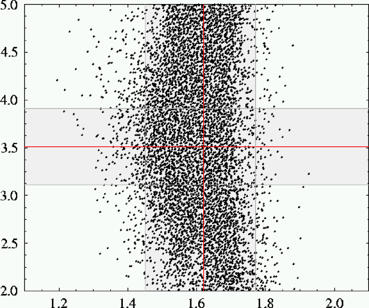
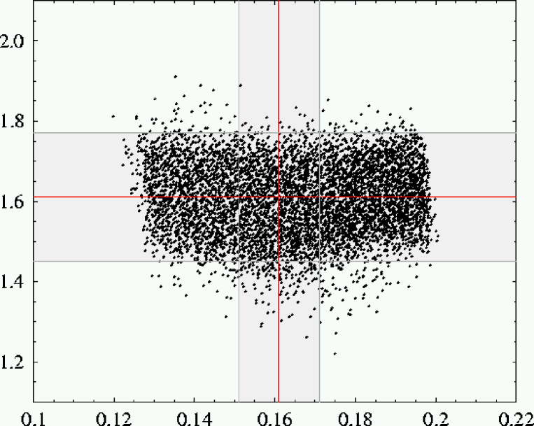
We find that the branching ratio ${Br}(\bar{B}\to X_{s}l^{+}l^{-})$ receives only small corrections within the considered MSSM scenario. This is illustrated in Fig. 4 where for randomly chosen points of the MSSM parameter space, fulfilling the lower sparticle mass bounds, the resulting ${Br}(\bar{B}\to X_{s}\gamma)$ versus ${Br}(\bar{B}\to X_{s}l^{+}l^{-})$ is shown. The vertical lines correspond to the SM prediction of ${Br}(\bar{B}\to X_{s}l^{+}l^{-})$ and the corresponding estimate of the theoretical uncertainty [22]. The horizontal lines indicate the SM prediction and theoretical uncertainties of ${Br}(\bar{B}\to X_{s}\gamma)$ [38, 16]. Deviations are possible from the SM central value ${Br}(\bar{B}\to X_{s}l^{+}l^{-})\sim 1.60\times 10^{-6}$ up to $\pm(15-20)\%$ respecting the experimental bound from ${Br}(\bar{B}\to X_{s}\gamma)$. Therefore the observable ${Br}(\bar{B}\to X_{s}l^{+}l^{-})$ of the low-$s$ region will not serve as a good candidate allowing to distinguish the SM and the considered MSSM scenario in view of the present theoretical uncertainties. The reason is the smallness of the MSSM contributions to $\widetilde{C}_{9}^{\rm{eff}}$ and $\widetilde{C}_{10}^{\rm{eff}}$ which dominate in the expression for ${Br}(\bar{B}\to X_{s}l^{+}l^{-})$ in the low-$s$ region. Although $\widetilde{C}_{7}^{\rm{eff}}$ could receive a larger MSSM contribution its magnitude is strongly constraint by the measured value of ${Br}(\bar{B}\to X_{s}\gamma)$. Furthermore, the contribution to $|\widetilde{C}_{7}^{\rm{eff}}|^{2}$ to the differential branching ratio falls like $1/\hat{s}$ and therefore only dominates for values of $\hat{s}\lesssim 0.05$ which coincides with the lower end of our integration range. The interplay between various contribution to the differential branching ratio within the SM is depicted in Fig. 7. There also a specific point in the space of supersymmetric parameters with significant corrections to $\widetilde{C}_{10}^{\rm{eff}}$ is shown.

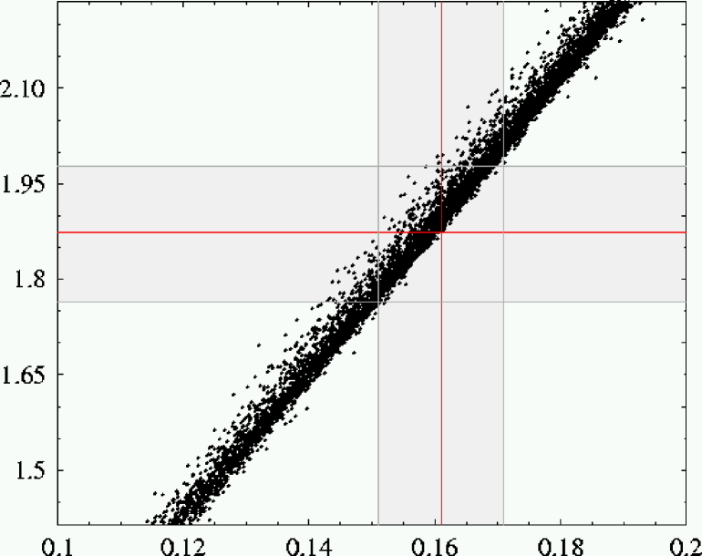
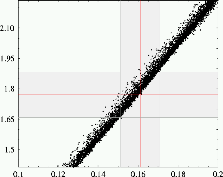
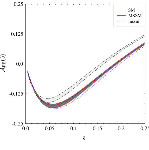
The position of the zero of the forward-backward asymmetry $\hat{s}_{0}$ represents a more sensitive observable than ${Br}(\bar{B}\to X_{s}l^{+}l^{-})$ in the considered MSSM scenario. In Fig. 5 we plot $\sqrt{{Br}(\bar{B}\to X_{s}\gamma)}$ versus $\hat{s}_{0}$ of the normalized $\bar{{\cal A}}_{\text{FB}}(\hat{s})$ for randomly chosen points of the MSSM parameter space. There the vertical lines correspond to the SM prediction of $\hat{s}_{0}$ and its uncertainties [22, 25] and the horizontal lines as in Fig. 4 to the SM prediction of ${Br}(\bar{B}\to X_{s}\gamma)$.

We note that the points in both plots in Fig. 5 are clustered along a straight line, exhibiting very clearly the correlation between the value of $Br(B\to X_{s}\gamma)$ and $\hat{s}_{0}$ within models with minimal flavour violation (MFV) as pointed out in [48].

The straight lines in Fig. 5 are to a very good approximation model independent within the class of models with MFV. Only different points on them correspond to different models and/or different sets of parameters in a given model. On the other hand the position of these lines depends on the parameters of the low energy theory, in particular on the charm quark mass that enters sensitively the evaluation of $Br(B\to X_{s}\gamma)$ [38] but is practically irrelevant for $\hat{s}_{0}$. In the left plot in Fig. 5 we used the $\overline{\rm MS}$ mass $\overline{m}_{c}(m_{c})$ and in the right plot the $m_{c}^{\rm pole}$ mass, that results in a different straight line. The SM prediction for ${Br}(\bar{B}\to X_{s}\gamma)$ is lower in the right plot than in the left plot. It is clear that the usefulness of the correlation between the values of $Br(B\to X_{s}\gamma)$ and $\hat{s}_{0}$ in testing the MSSM will depend on the progress in NNLO calculations for $B\to X_{s}\gamma$ that should significantly decrease the sensitivity due to the choice of $m_{c}$.

As seen in Fig. 5, in addition to dense points in the ballpark of SM expectations, there are values of $Br(B\to X_{s}\gamma)$ and $\hat{s}_{0}$ within the MSSM that are larger and smaller than the SM predictions. This should be contrasted with the result in a model with one universal extra dimension in which only smaller values of $Br(B\to X_{s}\gamma)$ and $\hat{s}_{0}$ were possible [48].

In Fig. 6 we show $Br(\bar{B}\to X_{s}l^{+}l^{-})$ versus $\hat{s}_{0}$. In the left plot the $\overline{\rm MS}$ definition was used for the charm quark mass in the evaluation of ${Br}(\bar{B}\to X_{s}\gamma)$ whereas in the right plot the pole-mass definition. As a consequence the allowed range of the position of the zero of $\bar{{\cal A}}_{\text{FB}}(\hat{s})$ becomes shifted a bit towards higher values. The comparison of Fig. 5 and 6 shows that the position of $\hat{s}_{0}$ is much more sensitive to the Wilson coefficient $C_{7}$ and consequently to $Br(B\to X_{s}\gamma)$ than to $Br(\bar{B}\to X_{s}l^{+}l^{-})$ itself.

“P1”	$M_{H}=440.11\,\mbox{GeV}$, $\tan\beta=5.01$, $\mu=-122.87\,\mbox{GeV}$, $M_{2}=184.56\,\mbox{GeV}$,
	$A_{U}={\rm diag}(370.29,\;79.60,\;535.71)\,\mbox{GeV}$,
	$M_{D_{L}}={\rm diag}(299.63,\;127.20,\;454.43)\,\mbox{GeV}$,
	$M_{U_{R}}={\rm diag}(219.96,\;519.91,\;167.68)\,\mbox{GeV}$
“P2”	$M_{H}=248.34\,\mbox{GeV}$, $\tan\beta=2.56$, $\mu=192.83\,\mbox{GeV}$, $M_{2}=489.68\,\mbox{GeV}$,
	$A_{U}={\rm diag}(-419.30,\;525.64,\;-540.81)\,\mbox{GeV}$,
	$M_{D_{L}}={\rm diag}(339.09,\;128.18,\;393.52)\,\mbox{GeV}$,
	$M_{U_{R}}={\rm diag}(232.08,\;351.41,\;234.77)\,\mbox{GeV}$
“P3”	$M_{H}=451.74\,\mbox{GeV}$, $\tan\beta=4.89$, $\mu=-540.06\,\mbox{GeV}$, $M_{2}=582.50\,\mbox{GeV}$,
	$A_{U}={\rm diag}(-375.95,\;-324.59,\;-497.23)\,\mbox{GeV}$,
	$M_{D_{L}}={\rm diag}(503.97,\;281.42,\;264.06)\,\mbox{GeV}$,
	$M_{U_{R}}={\rm diag}(444.06,\;186.86,\;417.40)\,\mbox{GeV}$.

Table 1: Three selected points. In all points $M_{\tilde{g}}=1\,\mbox{TeV}$, and the down-squarks and sneutrinos are assumed to have masses about $m_{\tilde{d}}=300\,\mbox{GeV}$ and $m_{\tilde{\nu}}=250\,\mbox{GeV}$.

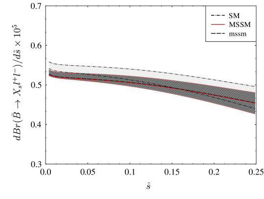
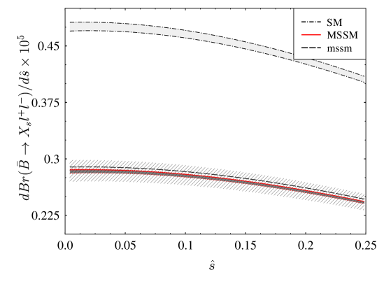
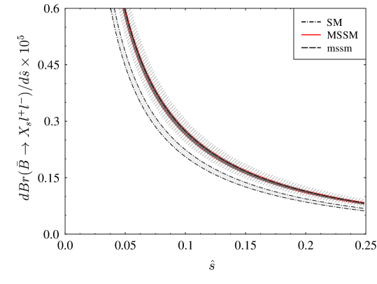
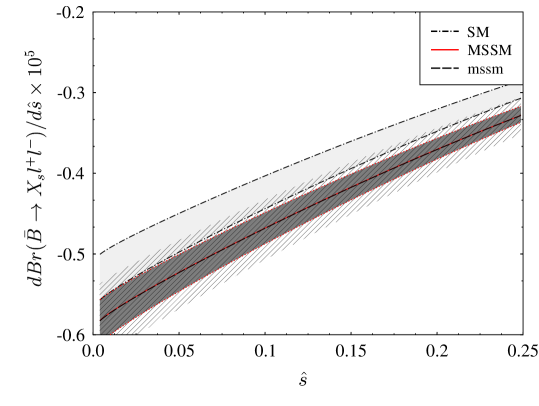
In Fig. 7 we show the four main contributions due to $|\widetilde{C}_{7,9,10}^{\rm{eff}}|^{2}$ and $\mbox{Re}\left(\widetilde{C}_{7}^{{\rm eff}}\widetilde{C}_{9}^{{\rm eff}*}\right)$ to the differential branching ratio, see (4.1), as functions of $\hat{s}$ for the fixed MSSM parameter point “P1” defined in Table 1. Each plot shows the SM (light grey band) and the MSSM contribution. To demonstrate the reduction of the renormalization scale dependence $\mu_{t}$ we show the MSSM result when including all calculated corrections (dark grey band – “MSSM”) and the partial MSSM result (shaded bend – “mssm”) obtained by discarding all contributions with $n=2$ and $i=\{H,{\tilde{\chi}},4\}$ to the functions $[X]^{n}_{i}$ in (3.7), but not to the SM. The bands are obtained by varying the renormalization scale $\mu_{t}\in[120,300]\,\mbox{GeV}$ and the low-energy scale $\mu_{b}\in[2.5,10]\,\mbox{GeV}$. Large deviations from the SM appear in the contribution $|\widetilde{C}_{10}^{\rm{eff}}|^{2}$ mainly due to the $Z^{0}$-penguin function $[C_{9}^{l\bar{l}}]$ which is suppressed in $|\widetilde{C}_{9}^{\rm{eff}}|^{2}$ as can be seen in (3). The inclusion of the NNLO matching conditions in the MSSM reduces the renormalization scale dependence to comparable size as obtained in the SM calculation.

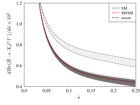
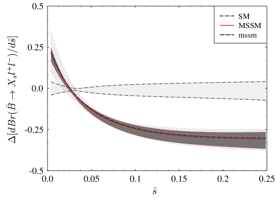
The sum of this four separate contributions (and the bremsstrahlung contributions) adds up to the final differential branching ratio shown in Fig. 8 in the left plot. As before the bands are obtained by variation of the renormalization scales $\mu_{t}$ and $\mu_{b}$. The reduction due to MSSM contributions is roughly $-30\%$ for values of $\hat{s}>0.15$ as can be seen in the right plot of Fig. 8 where the relative size compared to the SM result (obtained for $\mu_{t}=120\,\mbox{GeV}$ and $\mu_{b}=5\,\mbox{GeV}$) is given by the quantity $\Delta Q\equiv Q/Q_{\rm SM}-1$. Thus the shape and magnitude of the dilepton invariant mass distribution provides in certain regions of $\hat{s}$ a more sensitive observable then the integrated branching ratio itself in the search for deviations from the SM prediction, depending on the MSSM parameter point. It should be noted that the very small scale dependence around values of $\hat{s}\sim 0.05$ are due to accidental cancellations between the 4 separate contributions in (4.1).

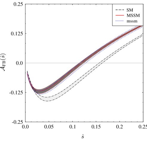
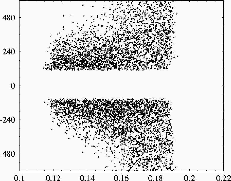
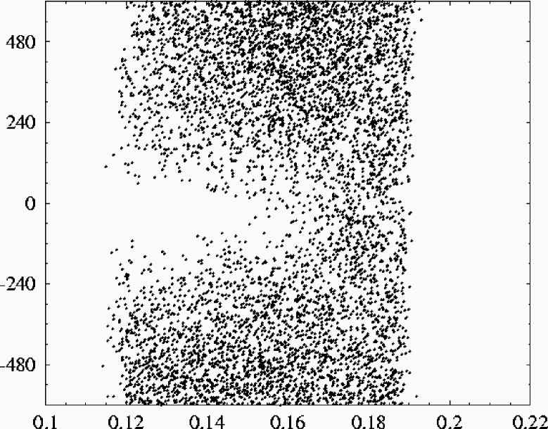
In Fig. 9 we show the normalized forward-backward asymmetry $\bar{{\cal A}}_{\text{FB}}(\hat{s})$ for the low-$s$ region. The left plot illustrates the result for the fixed MSSM-parameter point “P2” and the right plot for “P3” that are given in Table 1. The SM result is shown in both plots for comparison. Again the bands are obtained by varying the renormalization scales $\mu_{t}$ and $\mu_{b}$ as in Figs. 7 and  8. Due to the strong correlation of the position of the zero $\hat{s}_{0}$ and ${Br}(\bar{B}\to X_{s}\gamma)$ in the considered MSSM-scenarios further shifts to the left or right (as shown in the two plots) of $\hat{s}_{0}$ are unlikely.

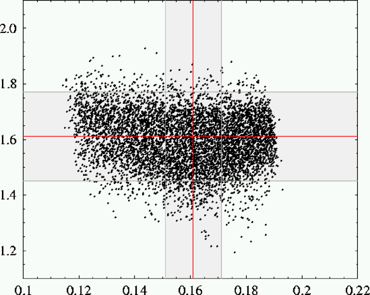
In Fig. 10 the fundamental MSSM parameters $\mu$ and $[A_{U}]_{33}$ are shown versus the position of the zero of $\bar{{\cal A}}_{\text{FB}}(\hat{s})$, $\hat{s}_{0}$, for the sample of random MSSM points given in Fig. 5. The lower and upper bounds of $\hat{s}_{0}$ present in both plots are evidently due to the strong correlation to ${Br}(\bar{B}\to X_{s}\gamma)$. The “hole” in the $\mu$ distribution for values $|\mu|<100\,\mbox{GeV}$ comes of course from the bound on the lightest chargino mass. As can be seen for small values of $\hat{s}_{0}$ also smaller values of $\mu$ are preferred. The allowed values of $[A_{U}]_{33}$ versus $\hat{s}_{0}$ generated during our random scan are shown in the right plot. Almost no bounds are found here, only towards smaller values of $\hat{s}_{0}$ very small values of $[A_{U}]_{33}$ seem to be excluded. We could not find such correlations for all other soft-SUSY breaking parameters.

6 Summary and Conclusions

In this paper we have presented for the first time complete NNLO QCD corrections to $\bar{B}\to X_{s}l^{+}l^{-}$ in the context of the MSSM within a scenario as defined in Section 2. We have calculated the missing ingredients of a complete NNLO result and including also contributions present already in the literature, we were able to calculate with this accuracy the branching ratio for $\bar{B}\to X_{s}l^{+}l^{-}$ in the low-$s$ region, the corresponding dilepton invariant mass distribution and the forward-backward asymmetry. The presented results can be applied to all MSSM scenarios with a flavour-diagonal down-squark mass-squared matrix, as long as the gluino is heavier compared to the remaining sparticle spectrum and $\tan\beta$ is small.

This calculation was motivated by the fact that in the SM the $\bar{B}\to X_{s}l^{+}l^{-}$ observables suffer from sizable renormalization scale uncertainties which are reduced considerably at NNLO. Consequently in order to have a chance to see supersymmetric effects of in this decay, it is essential to reduce renormalization scale uncertainties in the MSSM as well.

The results for the relevant Wilson coefficients are collected in Section 3 and the Appendix A, where we stated explicitly which corrections were already calculated previously and which are new. The numerical analysis of the quantities of interest is performed in Section 5. Our main findings are as follows:

• The $\mu$ dependence present in all quantities of interest at NLO is visibly reduced at NNLO depending on the magnitude of the MSSM contribution for the particular MSSM parameter point and it is typically of the same size as the one of the corresponding SM result.

• Supersymmetric effects in the branching ratio amount only to at most $20\%$ and consequently in view of theoretical uncertainties in this quantity it will be very difficult to see them unless experimental and theoretical uncertainties will be significantly reduced. In this respect the dilepton invariant mass distribution can offer in certain regions of $\hat{s}$ the possibility to distinguish the supersymmetric effects from the SM prediction. Such effects can reach up to $30\%$ depending on the MSSM parameters and the value of $\hat{s}$.

• The best chance to observe supersymmetric effects in this decays is through the forward-backward asymmetry. We find that the position of the zero $\hat{s}_{0}$ in this asymmetry can be significantly shifted both downwards and upwards relatively to the SM expectation. These shifts are accompanied by the shifts in ${Br}(\bar{B}\to X_{s}\gamma)$ as pointed out in [48] and shown in Fig. 5. As the predictions for $\hat{s}_{0}$ is theoretically rather clean, accurate measurements could be able to detect possible departure of its value from the SM prediction one day.

Acknowledgments

We thank Jörg Urban, Michael Spranger, Janusz Rosiek and Mikolaj Misiak for discussions. C.B. and T.E. have been supported by the German-Israeli Foundation under the contract G-698-22.7/2002. Further C.B. has been supported by the Department of Energy under Grant DE-FG03-97ER40546. The work presented here was also supported in part by the German Bundesministerium für Bildung und Forschung under the contract 05HT4WOA/3 and DFG Project Bu. 706/1-2.

Appendix A Wilson Coefficients

This appendix summarizes the matching results relevant for $\bar{B}\to X_{s}l^{+}l^{-}$ in the SM and the considered scenario of the MSSM as introduced in Section 2. It provides the formulae for the functions $[X]^{n}_{i}$ introduced in (3.7).

Dimensional regularization with fully anticommuting $\gamma_{5}$ and the $\overline{\rm MS}$ scheme was used for all QCD counterterms, both in the full and in the effective theory for light degrees of freedom. The only exceptions were the top quark and squark loop contributions to the renormalization of the light-quark and gluon wave functions on the full theory side. The corresponding terms in the propagators were subtracted in the MOM scheme at $q^{2}=0$. In consequence, no top quark and squark loop contribution remained in the “light quark – $W$ boson” effective vertex after renormalization.

The only relevant off-shell electroweak counterterm in the full theory proportional to $\bar{s}D\!\!\!\!/\,b$ was taken in the MOM scheme as well, at $q^{2}=0$ for the $\bar{s}\partial\!\!\!/b$, and at vanishing external momenta for terms containing gauge bosons.

As a consequence of this special choice of the renormalization, all masses of quarks and squarks, as well as the mixing matrix $\Gamma^{U}$ and the effective couplings $X_{i}^{U_{L}}$ and $X_{i}^{U_{R}}$ appearing in this Appendix are $\overline{\rm MS}$ quantities. The masses of particles which do not interact strongly are not renormalized and thus might be interpreted as their tree-level masses.

As already stated in Section 3 all the functions $[X]^{1}_{4}$ are equal to zero choosing an on-shell renormalization prescription for squark fields and masses [49] and the mixing matrix $\Gamma^{U}$ [50]. For example this can be seen by means of the following transformation formulae between $\overline{\rm MS}$ and on-shell scheme,

$$\quad m^{2}_{{\tilde{u}}_{a}}(\mu) =(m^{\rm pole}_{{\tilde{u}}_{a}})^{2}\Bigg{\{}1-\frac{\alpha_{s}(\mu)}{4\pi}\frac{4}{3}\left[7+3\ln\Bigg{(}\frac{\mu}{m^{\rm pole}_{{\tilde{u}}_{a}}}\Bigg{)}^{2}\right]$$

$$\hskip 71.13188pt+\frac{\alpha_{s}(\mu)}{4\pi}\frac{4}{3}\sum_{b=1}^{6}\frac{P^{U}_{ab}(m^{\rm pole}_{{\tilde{u}}_{b}})^{2}P^{U}_{ba}}{(m^{\rm pole}_{{\tilde{u}}_{a}})^{2}}\left[1+\ln\Bigg{(}\frac{\mu}{m^{\rm pole}_{{\tilde{u}}_{b}}}\Bigg{)}^{2}\right]\Bigg{\}},$$ (A.1)

$$\Gamma^{U}_{ab}(\mu) =\Gamma^{U}_{ab}+\frac{\alpha_{s}(\mu)}{4\pi}\frac{4}{3}\sum_{e=1}^{6}\sum_{\begin{subarray}{c}\scriptstyle c=1\\ \scriptstyle c\neq a\end{subarray}}^{6}\frac{P^{U}_{ae}(m^{\rm pole}_{{\tilde{u}}_{e}})^{2}P^{U}_{ec}}{(m^{\rm pole}_{{\tilde{u}}_{a}})^{2}-(m^{\rm pole}_{{\tilde{u}}_{c}})^{2}}\left[1+\ln\Bigg{(}\frac{\mu}{m^{\rm pole}_{{\tilde{u}}_{e}}}\Bigg{)}^{2}\right]\Gamma^{U}_{cb}.$$ (A.2)

On the left hand side of these equations the squark masses and the mixing matrix are running $\overline{\rm MS}$ parameters, whereas on the right hand side they take their on-shell values. We note that the couplings $a_{g}$ and $a_{Y}$ given in (2.3) are still $\overline{\rm MS}$ renormalized working with on-shell squark parameters.

We define the mass ratios

$$x =\frac{m_{t}^{2}}{M_{W}^{2}}, y =\frac{m_{t}^{2}}{M_{H}^{2}}, x_{ij} =\frac{M_{{\tilde{\chi}}_{i}}^{2}}{M_{{\tilde{\chi}}_{j}}^{2}}, y_{ai} =\frac{m_{{\tilde{u}}_{a}}^{2}}{M_{{\tilde{\chi}}_{i}}^{2}}, v_{fi} =\frac{m_{\tilde{\nu}_{f}}^{2}}{M_{{\tilde{\chi}}_{i}}^{2}},$$ (A.3)

and introduce the abbreviations

$$L_{t} =\ln\frac{\mu_{t}^{2}}{m_{t}^{2}}, L_{{\tilde{u}}_{a}} =\ln\frac{\mu_{t}^{2}}{m_{{\tilde{u}}_{a}}^{2}}, \kappa =\frac{1}{g_{2}^{2}V_{tb}V_{ts}^{\ast}}.$$ (A.4)

In these equations $m_{t}$ denotes the top quark mass, $m_{{\tilde{u}}_{a}}$ and $m_{{\tilde{d}}_{a}}$ up and down squark masses, $M_{W}$ the $W$ boson mass, $M_{H}$ the charged Higgs mass, $M_{{\tilde{\chi}}_{i}}$ the chargino masses and finally $m_{\tilde{\nu}_{f}}$ sneutrino masses.

The integral representations for the functions ${\rm Li}_{2}{\left(z\right)}$ and ${\rm Cl}_{2}{\left(x\right)}$ are as follows

$${\rm Li}_{2}{\left(z\right)} =-\int_{0}^{z}dt\frac{\ln(1-t)}{t},$$ (A.5)

$${\rm Cl}_{2}{\left(x\right)} ={\rm Im}\left[{\rm Li}_{2}{\left(e^{ix}\right)}\right]=-\int_{0}^{x}d\theta\ln|2\sin(\theta/2)|.$$ (A.6)

The calculation was performed in the background field formalism in an arbitrary $R_{\xi}$-gauge for the gluon gauge parameter and in the t‘Hooft-Feynman gauge for the $W$ boson gauge parameter.

Appendix A.1 $i=W$ – “top quark – W boson”

The evaluation of Feynman diagrams contributing to $b\to s+$(light particles) Greens functions within the SM mediated by “top quark – $W$ boson” loops yields the functions denoted by the index $i=W$ in (3.7). The explicit form can be found in [18] by using the equalities

$$\begin{array}[]{ccccc}{[A_{7}]}^{0}_{W}=A_{0}^{t}(x),&&{[B_{9}^{l\bar{l}}]}^{0}_{W}={[B_{10}^{l\bar{l}}]}^{0}_{W}=B_{0}^{t}(x),&&{[C_{9}^{l\bar{l}}]}^{0}_{W}=C_{0}^{t}(x),\\[11.38109pt] {[D_{9}]}^{0}_{W}=D_{0}^{t}(x),&&{[E_{4}]}^{0}_{W}=E_{0}^{t}(x),&&{[F_{8}]}^{0}_{W}=F_{0}^{t}(x),\\[11.38109pt] {[A_{7}]}^{1}_{W}=A_{1}^{t}(x),&&{[B_{9}^{l\bar{l}}]}^{1}_{W}={[B_{10}^{l\bar{l}}]}^{1}_{W}=B_{1}^{t}(x,-\frac{1}{2}),&&{[C_{9}^{l\bar{l}}]}^{1}_{W}=C_{1}^{t}(x),\\[11.38109pt] {[D_{9}]}^{1}_{W}=D_{1}^{t}(x),&&{[E_{4}]}^{1}_{W}=E_{1}^{t}(x),&&{[F_{8}]}^{1}_{W}=F_{1}^{t}(x),\\[11.38109pt] {[G_{3}]}^{1}_{W}=G_{1}^{t}(x).&&&&\end{array}$$ (A.7)

The functions $[X]^{1}_{W}$ have been first calculated in the following papers: $[A_{7}]^{1}_{W}$ and $[F_{8}]^{1}_{W}$ in [51, 52, 53, 54, 34], $[B_{9}^{l\bar{l}}]^{1}_{W}$ and $[C_{9}^{l\bar{l}}]^{1}_{W}$ in [55, 56, 57, 58] and $[D_{9}]^{1}_{W},\,[E_{4}]^{1}_{W}$ and $[G_{3}]^{1}_{W}$ in [18].

Appendix A.2 $i=H$ – “top quark – charged Higgs”

The evaluation of Feynman diagrams contributing to $b\to s+$(light particles) Greens functions within the MSSM (but also 2HDM of type II) mediated by “top quark – charged Higgs boson” loops and denoted by the index $i=H$ in (3.7) yields

$${[A_{7}]}^{0}_{H} =\textstyle\frac{-3y^{2}+2y}{3(y-1)^{3}}\ln y+\frac{5y^{2}-3y}{6(y-1)^{2}}+\cot^{2}\beta\left\{\frac{-3y^{3}+2y^{2}}{6(y-1)^{4}}\ln y+\frac{8y^{3}+5y^{2}-7y}{36(y-1)^{3}}\right\},$$ (A.8)

$${[B_{9}^{l\bar{l}}]}^{0}_{H} ={[B_{10}^{l\bar{l}}]}^{0}_{H}=0,$$ (A.9)

$${[C_{9}^{l\bar{l}}]}^{0}_{H} =\textstyle\frac{M_{H}^{2}}{8M_{W}^{2}}\cot^{2}\beta\left\{\frac{-y^{2}}{(y-1)^{2}}\ln y+\frac{y^{2}}{y-1}\right\},$$ (A.10)

$${[D_{9}]}^{0}_{H} =\textstyle\cot^{2}\beta\left\{\frac{-3y^{4}+6y^{2}-4y}{18(y-1)^{4}}\ln y+\frac{47y^{3}-79y^{2}+38y}{108(y-1)^{3}}\right\},$$ (A.11)

$${[E_{4}]}^{0}_{H} =\textstyle\cot^{2}\beta\left\{\frac{3y^{2}-2y}{6(y-1)^{4}}\ln y+\frac{7y^{3}-29y^{2}+16y}{36(y-1)^{3}}\right\},$$ (A.12)

$${[F_{8}]}^{0}_{H} =\textstyle\frac{y}{(y-1)^{3}}\ln y+\frac{y^{2}-3y}{2(y-1)^{2}}+\cot^{2}\beta\left\{\frac{y^{2}}{2(y-1)^{4}}\ln y+\frac{y^{3}-5y^{2}-2y}{12(y-1)^{3}}\right\},$$ (A.13)

$${[A_{7}]}^{1}_{H} =\textstyle\frac{-64y^{3}+224y^{2}-96y}{9(y-1)^{3}}{\rm Li}_{2}{\left(1-\frac{1}{y}\right)}+\frac{-28y^{3}+256y^{2}-132y}{9(y-1)^{4}}\ln y+\frac{16y^{3}-104y^{2}+56y}{3(y-1)^{3}}$$

$$\textstyle+\left[\frac{24y^{3}+112y^{2}-64y}{9(y-1)^{4}}\ln y+\frac{32y^{3}-188y^{2}+84y}{9(y-1)^{3}}\right]L_{t}$$

$$\textstyle+\cot^{2}\beta\left\{\frac{-32y^{4}+148y^{3}-72y^{2}}{9(y-1)^{4}}{\rm Li}_{2}{\left(1-\frac{1}{y}\right)}+\frac{-126y^{4}+1614y^{3}-926y^{2}+14y}{81(y-1)^{5}}\ln y\right.$$

$$\textstyle\left.+\frac{1202y^{4}-7569y^{3}+5436y^{2}-797y}{243(y-1)^{4}}+\left[\frac{12y^{4}+92y^{3}-56y^{2}}{9(y-1)^{5}}\ln y+\frac{28y^{4}-270y^{3}+36y^{2}+62y}{27(y-1)^{4}}\right]L_{t}\right\},$$ (A.14)

$${[B_{9}^{l\bar{l}}]}^{1}_{H} ={[B_{10}^{l\bar{l}}]}^{1}_{H}=0,$$ (A.15)

$${[C_{9}^{l\bar{l}}]}^{1}_{H} =\textstyle\frac{M_{H}^{2}}{8M_{W}^{2}}\cot^{2}\beta\left\{\frac{-8y^{3}+16y^{2}}{(y-1)^{2}}{\rm Li}_{2}{\left(1-\frac{1}{y}\right)}+\frac{-24y^{3}+88y^{2}}{3(y-1)^{3}}\ln y\right.+\frac{32y^{3}-96y^{2}}{3(y-1)^{2}}$$

$$\textstyle\left.+\left[\frac{16y^{2}}{(y-1)^{3}}\ln y+\frac{8y^{3}-24y^{2}}{(y-1)^{2}}\right]L_{t}\right\},$$ (A.16)

$${[D_{9}]}^{1}_{H} =\textstyle\cot^{2}\beta\left\{\frac{380y^{4}-528y^{3}+72y^{2}+128y}{81(y-1)^{4}}{\rm Li}_{2}{\left(1-\frac{1}{y}\right)}+\frac{596y^{4}-672y^{3}+64y^{2}+204y}{81(y-1)^{5}}\ln y\right.$$

$$\textstyle+\frac{-6175y^{4}+9138y^{3}-3927y^{2}-764y}{729(y-1)^{4}}$$

$$\textstyle\left.+\left[\frac{432y^{4}-456y^{3}+40y^{2}+128y}{81(y-1)^{5}}\ln y+\frac{-352y^{4}-972y^{3}+1944y^{2}-1052y}{243(y-1)^{4}}\right]L_{t}\right\},$$ (A.17)

$${[E_{4}]}^{1}_{H} =\textstyle\cot^{2}\beta\left\{\frac{515y^{4}-906y^{3}+99y^{2}+182y}{54(y-1)^{4}}{\rm Li}_{2}{\left(1-\frac{1}{y}\right)}+\frac{1030y^{4}-2763y^{3}-15y^{2}+980y}{108(y-1)^{5}}\ln y\right.$$

$$\textstyle+\frac{-29467y^{4}+68142y^{3}-6717y^{2}-18134y}{1944(y-1)^{4}}$$

$$\textstyle\left.+\left[\frac{-375y^{3}-95y^{2}+182y}{54(y-1)^{5}}\ln y+\frac{133y^{4}-108y^{3}+4023y^{2}-2320y}{324(y-1)^{4}}\right]L_{t}\right\},$$ (A.18)

$${[F_{8}]}^{1}_{H} =\textstyle\frac{-17y^{3}+25y^{2}-36y}{3(y-1)^{3}}{\rm Li}_{2}{\left(1-\frac{1}{y}\right)}+\frac{-34y^{3}+7y^{2}-165y}{6(y-1)^{4}}\ln y+\frac{29y^{3}-44y^{2}+143y}{4(y-1)^{3}}$$

$$\textstyle+\left[\frac{-34y^{2}-38y}{3(y-1)^{4}}\ln y+\frac{7y^{3}-16y^{2}+81y}{3(y-1)^{3}}\right]L_{t}$$

$$\textstyle+\cot^{2}\beta\left\{\frac{-13y^{4}+17y^{3}-30y^{2}}{3(y-1)^{4}}{\rm Li}_{2}{\left(1-\frac{1}{y}\right)}+\frac{-468y^{4}+321y^{3}-2155y^{2}-2y}{108(y-1)^{5}}\ln y\right.$$

$$\textstyle\left.+\frac{4451y^{4}-7650y^{3}+18153y^{2}-1130y}{648(y-1)^{4}}+\left[\frac{-17y^{3}-31y^{2}}{3(y-1)^{5}}\ln y+\frac{7y^{4}-18y^{3}+261y^{2}+38y}{18(y-1)^{4}}\right]L_{t}\right\},$$ (A.19)

$${[G_{3}]}^{1}_{H} =\textstyle\cot^{2}\beta\left\{\frac{10y^{4}+30y^{2}-20y}{27(y-1)^{4}}{\rm Li}_{2}{\left(1-\frac{1}{y}\right)}+\frac{30y^{3}-66y^{2}-56y}{81(y-1)^{4}}\ln y+\frac{6y^{3}-187y^{2}+213y}{81(y-1)^{3}}\right.$$

$$\textstyle\left.+\left[\frac{-30y^{2}+20y}{27(y-1)^{4}}\ln y+\frac{-35y^{3}+145y^{2}-80y}{81(y-1)^{3}}\right]L_{t}\right\}.$$ (A.20)

The following functions $[X]^{1}_{H}$ have been calculated previously: $[A_{7}]^{1}_{H}$ and $[F_{8}]^{1}_{H}$ in [53, 59, 34] and $[B_{10}^{l\bar{l}}]^{1}_{H}$ and $[C_{9}^{l\bar{l}}]^{1}_{H}$ in [33]. The function $[D_{9}]^{1}_{H}$ has been calculated in [36] and confirmed in [37]. The results for the functions $[E_{4}]^{1}_{H}$ and $[G_{3}]^{1}_{H}$ are new. Note that $[B_{9}^{l\bar{l}}]^{1}_{H}$ and $[B_{10}^{l\bar{l}}]^{1}_{H}$ vanish due to the approximation of vanishing lepton masses.

Appendix A.3 $i=\tilde{\chi}$ – “chargino – up squark”

The evaluation of Feynman diagrams contributing to $b\to s+$(light particles) Greens functions within the MSSM mediated by “chargino – up squark” loops and denoted by the index $i={\tilde{\chi}}$ in (3.7) yields

$${[A_{7}]}^{0}_{\tilde{\chi}} =\kappa\sum_{i=1}^{2}\sum_{a=1}^{6}\frac{M_{W}^{2}}{M_{{\tilde{\chi}}_{i}}^{2}}\left\{[{X_{i}^{U_{L}}}^{\dagger}]_{2a}[{X_{i}^{U_{L}}}]_{a3}\;h_{1}^{(0)}(y_{ai})+\frac{M_{{\tilde{\chi}}_{i}}}{m_{b}}[{X_{i}^{U_{L}}}^{\dagger}]_{2a}[{X_{i}^{U_{R}}}]_{a3}\;h_{2}^{(0)}(y_{ai})\right\},$$ (A.21)

$${[B_{9,10}^{l\bar{l}}]}^{0}_{\tilde{\chi}} =\mp\kappa\frac{M_{W}^{2}}{2g_{2}^{2}}\sum_{i,j=1}^{2}\sum_{a=1}^{6}\sum_{b=1}^{3}\frac{[{X_{j}^{U_{L}}}^{\dagger}]_{2a}[{X_{i}^{U_{L}}}]_{a3}}{M^{2}_{{\tilde{\chi}}_{i}}}$$

$$\times\left\{\frac{1}{2}[{X_{i}^{N_{L}}}^{\dagger}]_{lb}[{X_{j}^{N_{L}}}]_{bl}f_{5}^{(0)}(x_{ji},y_{ai},v_{bi})\mp[{X_{i}^{N_{R}}}^{\dagger}]_{lb}[{X_{j}^{N_{R}}}]_{bl}\sqrt{x_{ji}}f_{6}^{(0)}(x_{ji},y_{ai},v_{bi})\right\},$$ (A.22)

$${[C_{9}^{l\bar{l}}]}^{0}_{\tilde{\chi}} ={[C_{L}^{\nu\bar{\nu}}]}^{0}_{\tilde{\chi}},$$ (A.23)

$${[D_{9}]}^{0}_{\tilde{\chi}} =\kappa\sum_{i=1}^{2}\sum_{a=1}^{6}\frac{M_{W}^{2}}{M_{{\tilde{\chi}}_{i}}^{2}}[{X_{i}^{U_{L}}}^{\dagger}]_{2a}[{X_{i}^{U_{L}}}]_{a3}\;h_{3}^{(0)}(y_{ai}),$$ (A.24)

$${[E_{4}]}^{0}_{\tilde{\chi}} =\kappa\sum_{i=1}^{2}\sum_{a=1}^{6}\frac{M_{W}^{2}}{M_{{\tilde{\chi}}_{i}}^{2}}[{X_{i}^{U_{L}}}^{\dagger}]_{2a}[{X_{i}^{U_{L}}}]_{a3}\;h_{4}^{(0)}(y_{ai}),$$ (A.25)

$${[F_{8}]}^{0}_{\tilde{\chi}} =\kappa\sum_{i=1}^{2}\sum_{a=1}^{6}\frac{M_{W}^{2}}{M_{{\tilde{\chi}}_{i}}^{2}}\left\{[{X_{i}^{U_{L}}}^{\dagger}]_{2a}[{X_{i}^{U_{L}}}]_{a3}\;h_{5}^{(0)}(y_{ai})+\frac{M_{{\tilde{\chi}}_{i}}}{m_{b}}[{X_{i}^{U_{L}}}^{\dagger}]_{2a}[{X_{i}^{U_{R}}}]_{a3}\;h_{6}^{(0)}(y_{ai})\right\},$$ (A.26)

$${[A_{7}]}^{1}_{\tilde{\chi}} =\kappa\sum_{i=1}^{2}\sum_{a=1}^{6}\frac{M_{W}^{2}}{M_{{\tilde{\chi}}_{i}}^{2}}$$

$$\times\left\{[{X_{i}^{U_{L}}}^{\dagger}]_{2a}[{X_{i}^{U_{L}}}]_{a3}\;h_{1}^{(1)}(y_{ai},L_{{\tilde{u}}_{a}})+\frac{M_{{\tilde{\chi}}_{i}}}{m_{b}}[{X_{i}^{U_{L}}}^{\dagger}]_{2a}[{X_{i}^{U_{R}}}]_{a3}\;h_{2}^{(1)}(y_{ai},L_{{\tilde{u}}_{a}})\right\},$$ (A.27)

$${[B_{9,10}^{l\bar{l}}]}^{1}_{\tilde{\chi}} =\mp\kappa\frac{M_{W}^{2}}{2g_{2}^{2}}\sum_{i,j=1}^{2}\sum_{a=1}^{6}\sum_{b=1}^{3}\frac{[{X_{j}^{U_{L}}}^{\dagger}]_{2a}[{X_{i}^{U_{L}}}]_{a3}}{M^{2}_{{\tilde{\chi}}_{i}}}$$

$$\times\left\{\frac{1}{2}[{X_{i}^{N_{L}}}^{\dagger}]_{lb}[{X_{j}^{N_{L}}}]_{bl}\left[f_{8}^{(1)}(x_{ji},y_{ai},v_{bi})+4\left(1+y_{ai}\frac{\partial}{\partial y_{ai}}\right)f_{5}^{(0)}(x_{ji},y_{ai},v_{bi})\;L_{{\tilde{u}}_{a}}\right]\right.$$

$$\left.\quad\mp[{X_{i}^{N_{R}}}^{\dagger}]_{lb}[{X_{j}^{N_{R}}}]_{bl}\sqrt{x_{ji}}\left[f_{9}^{(1)}(x_{ji},y_{ai},v_{bi})+4\left(1+y_{ai}\frac{\partial}{\partial y_{ai}}\right)f_{6}^{(0)}(x_{ji},y_{ai},v_{bi})\;L_{{\tilde{u}}_{a}}\right]\right\},$$

$${[C_{9}^{l\bar{l}}]}^{1}_{\tilde{\chi}} ={[C_{L}^{\nu\bar{\nu}}]}^{1}_{\tilde{\chi}},$$ (A.29)

$${[D_{9}]}^{1}_{\tilde{\chi}} =\kappa\sum_{i=1}^{2}\sum_{a=1}^{6}\frac{M_{W}^{2}}{M_{{\tilde{\chi}}_{i}}^{2}}[{X_{i}^{U_{L}}}^{\dagger}]_{2a}[{X_{i}^{U_{L}}}]_{a3}\;h_{3}^{(1)}(y_{ai},L_{{\tilde{u}}_{a}}),$$ (A.30)

$${[E_{4}]}^{1}_{\tilde{\chi}} =\kappa\sum_{i=1}^{2}\sum_{a=1}^{6}\frac{M_{W}^{2}}{M_{{\tilde{\chi}}_{i}}^{2}}[{X_{i}^{U_{L}}}^{\dagger}]_{2a}[{X_{i}^{U_{L}}}]_{a3}\;h_{4}^{(1)}(y_{ai},L_{{\tilde{u}}_{a}}),$$ (A.31)

$${[F_{8}]}^{1}_{\tilde{\chi}} =\kappa\sum_{i=1}^{2}\sum_{a=1}^{6}\frac{M_{W}^{2}}{M_{{\tilde{\chi}}_{i}}^{2}}$$

$$\times\left\{[{X_{i}^{U_{L}}}^{\dagger}]_{2a}[{X_{i}^{U_{L}}}]_{a3}\;h_{5}^{(1)}(y_{ai},L_{{\tilde{u}}_{a}})+\frac{M_{{\tilde{\chi}}_{i}}}{m_{b}}[{X_{i}^{U_{L}}}^{\dagger}]_{2a}[{X_{i}^{U_{R}}}]_{a3}\;h_{6}^{(1)}(y_{ai},L_{{\tilde{u}}_{a}})\right\},$$ (A.32)

$${[G_{3}]}^{1}_{\tilde{\chi}} =\kappa\sum_{i=1}^{2}\sum_{a=1}^{6}\frac{M_{W}^{2}}{M_{{\tilde{\chi}}_{i}}^{2}}[{X_{i}^{U_{L}}}^{\dagger}]_{2a}[{X_{i}^{U_{L}}}]_{a3}\;h_{7}^{(1)}(y_{ai},L_{{\tilde{u}}_{a}}).$$ (A.33)

The following functions $[X]^{1}_{\tilde{\chi}}$ have been calculated previously: $[A_{7}]^{1}_{\tilde{\chi}}$ and $[F_{8}]^{1}_{\tilde{\chi}}$ in [42, 34] and $[B_{10}^{l\bar{l}}]^{1}_{\tilde{\chi}}$ and $[C_{9}^{l\bar{l}}]^{1}_{\tilde{\chi}}$ in [33]. The results for the functions $[B_{9}^{l\bar{l}}]^{1}_{\tilde{\chi}}$, $[D_{9}]^{1}_{\tilde{\chi}},\,[E_{4}]^{1}_{\tilde{\chi}}$ and $[G_{3}]^{1}_{\tilde{\chi}}$ are new. The expressions for the functions ${[C_{L}^{\nu\bar{\nu}}]}^{0}_{\tilde{\chi}}$ and ${[C_{L}^{\nu\bar{\nu}}]}^{1}_{\tilde{\chi}}$ correspond to the leading and the next-to leading contributions to the function ${[C_{L}^{\nu\bar{\nu}}]}_{\tilde{\chi}}={[C_{L}^{\nu\bar{\nu}}]}^{0}_{\tilde{\chi}}+\alpha_{s}/(4\pi){[C_{L}^{\nu\bar{\nu}}]}^{1}_{\tilde{\chi}}$ given in (3.14) of [33].

Appendix A.4 $i=4$ – “chargino – up squark (quartic)”

The evaluation of Feynman diagrams contributing to $b\to s+$(light particles) Greens functions within the MSSM mediated by “chargino – up squark” loops containing the quartic squark vertex instead of gluon corrections and denoted by the index $i=4$ in (3.7) yields

$${[A_{7}]}^{1}_{4} =\kappa\sum_{i=1}^{2}\sum_{a,b,c=1}^{6}\frac{M_{W}^{2}}{M_{{\tilde{\chi}}_{i}}^{2}}\;P^{U}_{ab}\,y_{bi}\,P^{U}_{bc}\;(1+L_{{\tilde{u}}_{b}})$$

$$\times\left\{[{X_{i}^{U_{L}}}^{\dagger}]_{2a}[{X_{i}^{U_{L}}}]_{c3}\;[-q_{1}^{(1)}(y_{ai},y_{ci})+\frac{2}{3}q_{2}^{(1)}(y_{ai},y_{ci})]\right.$$

$$\left.\quad+\frac{M_{{\tilde{\chi}}_{i}}}{m_{b}}[{X_{i}^{U_{L}}}^{\dagger}]_{2a}[{X_{i}^{U_{R}}}]_{c3}\;[-q_{3}^{(1)}(y_{ai},y_{ci})+\frac{2}{3}q_{4}^{(1)}(y_{ai},y_{ci})]\right\},$$ (A.34)

$${[B_{9,10}^{l\bar{l}}]}^{1}_{4} =\pm\frac{\kappa}{2g_{2}^{2}}\frac{4}{3}\sum_{i,j=1}^{2}\sum_{f=1}^{3}\sum_{a,b,c=1}^{6}\frac{M_{W}^{2}}{M_{\tilde{\chi}_{i}}^{2}}\;P^{U}_{ab}\,y_{bi}\,P^{U}_{bc}\;(1+L_{\tilde{u}_{b}})\;[{X_{j}^{U_{L}}}^{\dagger}]_{2a}[{X_{i}^{U_{L}}}]_{c3}$$

$$\times\left\{\frac{1}{2}f^{(0)}_{9}(x_{ji},y_{ai},y_{ci},v_{fi})[{X_{i}^{N_{L}}}^{\dagger}]_{lf}[{X_{j}^{N_{L}}}]_{fl}\right.$$

$$\left.\qquad\mp\sqrt{x_{ji}}f^{(0)}_{10}(x_{ji},y_{ai},y_{ci},v_{fi})[{X_{i}^{N_{R}}}^{\dagger}]_{lf}[{X_{j}^{N_{R}}}]_{fl}\right\},$$ (A.35)

$${[C_{9}^{l\bar{l}}]}^{1}_{4} =\frac{\kappa}{6}\sum_{i,j=1}^{2}\sum_{a,\dots,e,g,k=1}^{6}P^{U}_{gk}\,y_{ki}\,P^{U}_{ke}\;(1+L_{\tilde{u}_{k}})\;[{X_{j}^{U_{L}}}^{\dagger}]_{2d}[{X_{i}^{U_{L}}}]_{a3}$$

$$\times\Bigg{\{}2\sqrt{x_{ji}}f_{6}^{(0)}(x_{ji},y_{ai},y_{di})U_{j1}U_{i1}^{\ast}\delta_{ae}\delta_{gd}\delta_{b1}\delta_{c1}-f_{5}^{(0)}(x_{ji},y_{ai},y_{di})V_{j1}^{\ast}V_{i1}\delta_{ae}\delta_{gd}\delta_{b1}\delta_{c1}$$

$$+f_{5}^{(0)}(y_{ai},y_{bi},y_{ci})(\Gamma^{U_{L}}{\Gamma^{U_{L}\dagger}})_{cb}\delta_{ij}\delta_{ae}\delta_{bg}\delta_{cd}+f_{5}^{(0)}(y_{ai},y_{ci},y_{di})(\Gamma^{U_{L}}{\Gamma^{U_{L}\dagger}})_{cb}\delta_{ij}\delta_{ab}\delta_{ce}\delta_{dg}\Bigg{\}},$$ (A.36)

$${[D_{9}]}^{1}_{4} =\kappa\sum_{i=1}^{2}\sum_{a,b,c=1}^{6}\frac{M_{W}^{2}}{M_{{\tilde{\chi}}_{i}}^{2}}\;P^{U}_{ab}\,y_{bi}\,P^{U}_{bc}\;(1+L_{{\tilde{u}}_{b}})\;[{X_{i}^{U_{L}}}^{\dagger}]_{2a}[{X_{i}^{U_{L}}}]_{c3}\;q_{5}^{(1)}(y_{ai},y_{ci}),$$ (A.37)

$${[E_{4}]}^{1}_{4} =\kappa\sum_{i=1}^{2}\sum_{a,b,c=1}^{6}\frac{M_{W}^{2}}{M_{{\tilde{\chi}}_{i}}^{2}}\;P^{U}_{ab}\,y_{bi}\,P^{U}_{bc}\;(1+L_{{\tilde{u}}_{b}})\;[{X_{i}^{U_{L}}}^{\dagger}]_{2a}[{X_{i}^{U_{L}}}]_{c3}\;q_{6}^{(1)}(y_{ai},y_{ci}),$$ (A.38)

$${[F_{8}]}^{1}_{4} =\kappa\sum_{i=1}^{2}\sum_{a,b,c=1}^{6}\frac{M_{W}^{2}}{M_{{\tilde{\chi}}_{i}}^{2}}\;P^{U}_{ab}y_{bi}\,P^{U}_{bc}\;(1+L_{{\tilde{u}}_{b}})\;$$

$$\times\left\{[{X_{i}^{U_{L}}}^{\dagger}]_{2a}[{X_{i}^{U_{L}}}]_{c3}\;q_{2}^{(1)}(y_{ai},y_{ci})+\frac{M_{{\tilde{\chi}}_{i}}}{m_{b}}[{X_{i}^{U_{L}}}^{\dagger}]_{2a}[{X_{i}^{U_{R}}}]_{c3}\;q_{4}^{(1)}(y_{ai},y_{ci})\right\},$$ (A.39)

$${[G_{3}]}^{1}_{4} =0.$$ (A.40)

The following functions $[X]^{1}_{4}$ have been calculated previously: $[A_{7}]^{1}_{4}$ and $[F_{8}]^{1}_{4}$ in [34] and $[B_{10}^{l\bar{l}}]^{1}_{4}$ and $[C_{9}^{l\bar{l}}]^{1}_{4}$ in [33]. The result for the functions $[B_{9}^{l\bar{l}}]^{1}_{4}$, $[D_{9}]^{1}_{4},\,[E_{4}]^{1}_{4}$ and $[G_{3}]^{1}_{4}$ are new.

Appendix B Auxiliary functions

Here we present explicit formulae for the loop functions $h_{i}^{(0)}(x)$, $h_{i}^{(1)}(x)$ and $q_{i}^{(1)}(x,y)$ introduced in Appendix A. They read

$$h_{1}^{(0)}(x) =\textstyle\frac{3x^{2}-2x}{3(x-1)^{4}}\ln x+\frac{-8x^{2}-5x+7}{18(x-1)^{3}},$$ (B.41)

$$h_{2}^{(0)}(x) =\textstyle\frac{-6x^{2}+4x}{3(x-1)^{3}}\ln x+\frac{7x-5}{3(x-1)^{2}},$$ (B.42)

$$h_{3}^{(0)}(x) =\textstyle\frac{-6x^{3}+9x^{2}-2}{9(x-1)^{4}}\ln x+\frac{52x^{2}-101x+43}{54(x-1)^{3}},$$ (B.43)

$$h_{4}^{(0)}(x) =\textstyle\frac{-1}{3(x-1)^{4}}\ln x+\frac{2x^{2}-7x+11}{18(x-1)^{3}},$$ (B.44)

$$h_{5}^{(0)}(x) =\textstyle\frac{-x}{(x-1)^{4}}\ln x+\frac{-x^{2}+5x+2}{6(x-1)^{3}},$$ (B.45)

$$h_{6}^{(0)}(x) =\textstyle\frac{2x}{(x-1)^{3}}\ln x+\frac{-x-1}{(x-1)^{2}},$$ (B.46)

$$h_{1}^{(1)}(x,y) =\textstyle\frac{-48x^{3}-104x^{2}+64x}{9(x-1)^{4}}{\rm Li}_{2}{\left(1-\frac{1}{x}\right)}+\frac{-378x^{3}-1566x^{2}+850x+86}{81(x-1)^{5}}\ln x$$

$$\textstyle+\frac{2060x^{3}+3798x^{2}-2664x-170}{243(x-1)^{4}}+\left[\frac{12x^{3}-124x^{2}+64x}{9(x-1)^{5}}\ln x+\frac{-56x^{3}+258x^{2}+24x-82}{27(x-1)^{4}}\right]y,$$ (B.47)

$$h_{2}^{(1)}(x,y) =\textstyle\frac{224x^{2}-96x}{9(x-1)^{3}}{\rm Li}_{2}{\left(1-\frac{1}{x}\right)}+\frac{-24x^{3}+352x^{2}-128x-32}{9(x-1)^{4}}\ln x+\frac{-340x^{2}+132x+40}{9(x-1)^{3}}$$

$$\textstyle+\left[\frac{-24x^{3}+176x^{2}-80x}{9(x-1)^{4}}\ln x+\frac{-28x^{2}-108x+64}{9(x-1)^{3}}\right]y,$$ (B.48)

$$h_{3}^{(1)}(x,y) =\textstyle\frac{32x^{3}+120x^{2}-384x+128}{81(x-1)^{4}}{\rm Li}_{2}{\left(1-\frac{1}{x}\right)}+\frac{-108x^{4}+1058x^{3}-898x^{2}-1098x+710}{81(x-1)^{5}}\ln x$$

$$\textstyle+\frac{-304x^{3}-13686x^{2}+29076x-12062}{729(x-1)^{4}}$$

$$\textstyle+\left[\frac{540x^{3}-972x^{2}+232x+56}{81(x-1)^{5}}\ln x+\frac{-664x^{3}+54x^{2}+1944x-902}{243(x-1)^{4}}\right]y,$$ (B.49)

$$h_{4}^{(1)}(x,y) =\textstyle\frac{-562x^{3}+1101x^{2}-420x+101}{54(x-1)^{4}}{\rm Li}_{2}{\left(1-\frac{1}{x}\right)}+\frac{-562x^{3}+1604x^{2}-799x+429}{54(x-1)^{5}}\ln x$$

$$\textstyle+\frac{17470x^{3}-47217x^{2}+31098x-13447}{972(x-1)^{4}}+\left[\frac{89x+55}{27(x-1)^{5}}\ln x+\frac{38x^{3}-135x^{2}+54x-821}{162(x-1)^{4}}\right]y,$$ (B.50)

$$h_{5}^{(1)}(x,y) =\textstyle\frac{9x^{3}+46x^{2}+49x}{6(x-1)^{4}}{\rm Li}_{2}{\left(1-\frac{1}{x}\right)}+\frac{81x^{3}+594x^{2}+1270x+71}{54(x-1)^{5}}\ln x$$

$$\textstyle+\frac{-923x^{3}-3042x^{2}-6921x-1210}{324(x-1)^{4}}+\left[\frac{10x^{2}+38x}{3(x-1)^{5}}\ln x+\frac{-7x^{3}+30x^{2}-141x-26}{9(x-1)^{4}}\right]y,$$ (B.51)

$$h_{6}^{(1)}(x,y) =\textstyle\frac{-32x^{2}-24x}{3(x-1)^{3}}{\rm Li}_{2}{\left(1-\frac{1}{x}\right)}+\frac{-52x^{2}-109x-7}{3(x-1)^{4}}\ln x+\frac{95x^{2}+180x+61}{6(x-1)^{3}}$$

$$\textstyle+\left[\frac{-20x^{2}-52x}{3(x-1)^{4}}\ln x+\frac{-2x^{2}+60x+14}{3(x-1)^{3}}\right]y,$$ (B.52)

$$h_{7}^{(1)}(x,y) =\textstyle\frac{-20x^{3}+60x^{2}-60x-20}{27(x-1)^{4}}{\rm Li}_{2}{\left(1-\frac{1}{x}\right)}+\frac{-60x^{2}+240x+4}{81(x-1)^{4}}\ln x+\frac{132x^{2}-382x+186}{81(x-1)^{3}}$$

$$\textstyle+\left[\frac{20}{27(x-1)^{4}}\ln x+\frac{-20x^{2}+70x-110}{81(x-1)^{3}}\right]y,$$ (B.53)

$$q_{1}^{(1)}(x,y) =\textstyle\frac{4}{3(x-y)}\left[\frac{x^{2}\ln x}{(x-1)^{4}}-\frac{y^{2}\ln y}{(y-1)^{4}}\right]+\frac{4x^{2}y^{2}+10xy^{2}-2y^{2}+10x^{2}y-44xy+10y-2x^{2}+10x+4}{9(x-1)^{3}(y-1)^{3}},$$ (B.54)

$$q_{2}^{(1)}(x,y) =\textstyle\frac{4}{3(x-y)}\left[\frac{x\ln x}{(x-1)^{4}}-\frac{y\ln y}{(y-1)^{4}}\right]+\frac{-2x^{2}y^{2}+10xy^{2}+4y^{2}+10x^{2}y-20xy-14y+4x^{2}-14x+22}{9(x-1)^{3}(y-1)^{3}},$$ (B.55)

$$q_{3}^{(1)}(x,y) =\textstyle\frac{8}{3(x-y)}\left[\frac{-x^{2}\ln x}{(x-1)^{3}}+\frac{y^{2}\ln y}{(y-1)^{3}}\right]+\frac{-12xy+4y+4x+4}{3(x-1)^{2}(y-1)^{2}},$$ (B.56)

$$q_{4}^{(1)}(x,y) =\textstyle\frac{8}{3(x-y)}\left[\frac{-x\ln x}{(x-1)^{3}}+\frac{y\ln y}{(y-1)^{3}}\right]+\frac{-4xy-4y-4x+12}{3(x-1)^{2}(y-1)^{2}},$$ (B.57)

$$q_{5}^{(1)}(x,y) =\textstyle\frac{4}{27(x-y)}\left[\frac{(6x^{3}-9x^{2}+2)\ln x}{(x-1)^{4}}-\frac{(6y^{3}-9y^{2}+2)\ln y}{(y-1)^{4}}\right]$$

$$\textstyle+\frac{104x^{2}y^{2}-202xy^{2}+86y^{2}-202x^{2}y+380xy-154y+86x^{2}-154x+56}{81(x-1)^{3}(y-1)^{3}},$$ (B.58)

$$q_{6}^{(1)}(x,y) =\textstyle\frac{4}{9(x-y)}\left[\frac{\ln x}{(x-1)^{4}}-\frac{\ln y}{(y-1)^{4}}\right]+\frac{4x^{2}y^{2}-14xy^{2}+22y^{2}-14x^{2}y+52xy-62y+22x^{2}-62x+52}{27(x-1)^{3}(y-1)^{3}}.$$ (B.59)

The functions $f^{(0)}_{5}$, $f^{(0)}_{6}$, $f^{(0)}_{9}$, $f^{(0)}_{10}$, $f^{(1)}_{8}$ and $f^{(1)}_{9}$ can be found in Appendix B of [33].

References

- [1]
- [2] J. Kaneko et al. [Belle Collaboration], Phys. Rev. Lett. 90 (2003) 021801, hep-ex/0208029; hep-ex/0408119.
- [3] B. Aubert et al. [BaBar Collaboration], hep-ex/0308016; Phys. Rev. Lett. 93 (2004) 081802, hep-ex/0404006.
- [4] Z. Ligeti and M. B. Wise, Phys. Rev. D53 (1996) 4937, hep-ph/9512225.
- [5] G. Buchalla and G. Isidori, Nucl. Phys. B525 (1998) 333, hep-ph/9801456.
- [6] A. F. Falk, M. E. Luke and M. J. Savage, Phys. Rev. D49 (1994) 3367, hep-ph/9308288.
- [7] A. Ali, G. Hiller, L. T. Handoko and T. Morozumi, Phys. Rev. D55 (1997) 4105, hep-ph/9609449.
- [8] J. W. Chen, G. Rupak and M. J. Savage, Phys. Lett. B410 (1997) 285, hep-ph/9705219.
- [9] C. W. Bauer and C. N. Burrell, Phys. Lett. B469 (1999) 248, hep-ph/9907517; Phys. Rev. D62 (2000) 114028, hep-ph/9911404.
- [10] G. Buchalla, G. Isidori and S. J. Rey, Nucl. Phys. B511 (1998) 594, hep-ph/9705253.
- [11] B. Grinstein, M. J. Savage and M. B. Wise, Nucl. Phys. B319 (1989) 271.
- [12] R. Grigjanis, P. J. O’Donnell, M. Sutherland and H. Navelet, Phys. Lett. B223 (1989) 239.
- [13] G. Cella, G. Ricciardi and A. Vicere, Phys. Lett. B258 (1991) 212.
- [14] M. Misiak, Nucl. Phys. B393 (1993) 23, Erratum: Nucl. Phys. B439 (1995) 461.
- [15] A. J. Buras and M. Münz, Phys. Rev. D52 (1995) 186, hep-ph/9501281.
- [16] A. J. Buras, A. Czarnecki, M. Misiak and J. Urban, Nucl. Phys. B631 (2002) 219, hep-ph/0203135.
- [17] H. M. Asatrian, H. H. Asatryan and A. Hovhannisyan, hep-ph/0401038.
- [18] C. Bobeth, M. Misiak and J. Urban, Nucl. Phys. B574 (2000) 291, hep-ph/9910220.
- [19] K. G. Chetyrkin, M. Misiak and M. Münz, Phys. Lett. B400 (1997) 206, Erratum Phys. Lett. B425 (1998) 414, hep-ph/9612313.
- [20] P. Gambino, M. Gorbahn and U. Haisch, Nucl. Phys. B673 (2003) 238, hep-ph/0306079.
- [21] M. Gorbahn and U. Haisch, in preparation.
- [22] C. Bobeth, P. Gambino, M. Gorbahn and U. Haisch, JHEP 0404 (2004) 071, hep-ph/0312090.
- [23] H. H. Asatrian, H. M. Asatrian, C. Greub and M. Walker, Phys. Lett. B507 (2001) 162, hep-ph/0103087; Phys. Rev. D65 (2002) 074004, hep-ph/0109140.
- [24] H. H. Asatrian, H. M. Asatrian, C. Greub and M. Walker, Phys. Rev. D66 (2002) 034009, hep-ph/0204341.
- [25] A. Ghinculov, T. Hurth, G. Isidori and Y. P. Yao, Nucl. Phys. B685 (2004) 351, hep-ph/0312128.
- [26] A. Ali, E. Lunghi, C. Greub and G. Hiller, Phys. Rev. D66 (2002) 034002, hep-ph/0112300.
- [27] G. Burdman, Phys. Rev. D52 (1995) 6400, hep-ph/9505352; Phys. Rev. D57 (1998) 4254, hep-ph/9710550.
- [28] A. Ghinculov, T. Hurth, G. Isidori and Y.-P. Yao, Nucl. Phys. B648 (2003) 254, hep-ph/0208088.
- [29] H. M. Asatrian, K. Bieri, C. Greub and A. Hovhannisyan, Phys. Rev. D66 (2002) 094013, hep-ph/0209006.
- [30] H. M. Asatrian, H. H. Asatryan, A. Hovhannisyan and V. Poghosyan, Mod. Phys. Lett. A19 (2004) 603, hep-ph/0311187.
- [31] C. Bobeth, T. Ewerth, F. Krüger and J. Urban, Phys. Rev. D66 (2002) 074021, hep-ph/0204225.
- [32] A. J. Buras, P. H. Chankowski, J. Rosiek and L. Slawianowska, Phys. Lett. B546 (2002) 96, hep-ph/0207241; Nucl. Phys. B659 (2003) 3, hep-ph/0210145.
- [33] C. Bobeth, A. J. Buras, F. Krüger and J. Urban, Nucl. Phys. B630 (2002) 87, hep-ph/0112305.
- [34] C. Bobeth, M. Misiak and J. Urban, Nucl. Phys. B567 (2000) 153, hep-ph/9904413.
- [35] A. J. Buras, hep-ph/9806471 (“Les Houches Lectures 1997”); G. Buchalla, A. J. Buras and M. E. Lautenbacher, Rev. Mod. Phys 68, 1125 (1996), hep-ph/9512380.
- [36] C. Bobeth, PhD, TU Munich, August, 2003.
- [37] S. Schilling, C. Greub, N. Salzmann and B. Toedtli, hep-ph/0407323.
- [38] P. Gambino and M. Misiak, Nucl. Phys. B611 (2001) 338, hep-ph/0104034.
- [39] P. H. Chankowski and L. Slawianowska, Eur. Phys. J. C33 (2004) 123, hep-ph/0308032.
- [40] M. Misiak, S. Pokorski and J. Rosiek, Adv. Ser. Direct. High Energy Phys. 15 (1998) 795, hep-ph/9703442.
- [41] S. Eidelman et al. [Particle Data Group Collaboration], Phys. Lett. B592 (2004) 1.
- [42] M. Ciuchini, G. Degrassi, P. Gambino and G. F. Giudice, Nucl. Phys. B534 (1998) 3, hep-ph/9806308.
- [43] K. Bieri, C. Greub and M. Steinhauser, Phys. Rev. D67 (2003) 114019, hep-ph/0302051; M. Misiak and M. Steinhauser, Nucl. Phys. B683 (2004) 277, hep-ph/0401041.
- [44] C. Jessop, SLAC-PUB-9610, (2002).
- [45] P. Koppenburg et al. [Belle Collaboration], Phys. Rev. Lett. 93 (2004) 061803, hep-ex/0403004.
- [46] M. Neubert, hep-ph/0408179.
- [47] G. Hiller and F. Krüger, Phys. Rev. D69 (2004) 074020, hep-ph/0310219.
- [48] A. J. Buras, A. Poschenrieder, M. Spranger and A. Weiler, Nucl. Phys. B678 (2004) 455, hep-ph/0306158.
- [49] K. I. Aoki, Z. Hioki, M. Konuma, R. Kawabe and T. Muta, Prog. Theor. Phys. Suppl. 73 (1982) 1; M. Böhm, H. Spiesberger and W. Hollik, Fortsch. Phys. 34 (1986) 687; A. Denner, Fortsch. Phys. 41 (1993) 307.
- [50] See for example Y. Yamada, Phys. Rev. D64 (2001) 036008, hep-ph/0103046, and references therein.
- [51] K. Adel and Y. P. Yao, Phys. Rev. D49 (1994) 4945, hep-ph/9308349.
- [52] C. Greub and T. Hurth, Phys. Rev. D56 (1997) 2934, hep-ph/9703349.
- [53] M. Ciuchini, G. Degrassi, P. Gambino and G. F. Giudice, Nucl. Phys. B527 (1998) 21, hep-ph/9710335.
- [54] A. J. Buras, A. Kwiatkowski and N. Pott, Nucl. Phys. B517 (1998) 353, hep-ph/9710336.
- [55] G. Buchalla and A. J. Buras, Nucl. Phys. B398 (1993) 285.
- [56] G. Buchalla and A. J. Buras, Nucl. Phys. B400 (1993) 225.
- [57] G. Buchalla and A. J. Buras, Nucl. Phys. B548 (1999) 309, hep-ph/9901288.
- [58] M. Misiak and J. Urban, Phys. Lett. B451 (1999) 161, hep-ph/9901278.
- [59] F. Borzumati and C. Greub, Phys. Rev. D58 (1998) 074004, hep-ph/9802391; Addendum: Phys. Rev. D59 (1999) 057501, hep-ph/9809438.