BUHEP-04-12

UMD-PP-05-017

^aPhysics Department, University of Maryland
College Park, Maryland 20742

^bPhysics Department, Boston University
Boston, Massachusetts 02215

^cJefferson Laboratory of Physics, Harvard University
Cambridge, Massachusetts 02138

We point out that the flavor problem in theories with dynamical electroweak symmetry breaking can be effectively decoupled if the physics above the TeV scale is strongly conformal, and the electroweak order parameter has a scaling dimension $d=1+\epsilon$ with $\epsilon\simeq 1/{\rm few}$. There are many restrictions on small values of $\epsilon$: for $\epsilon\ll 1$, electroweak symmetry breaking requires a fine-tuning similar to that of the standard model; large-$N$ conformal field theories (including those obtained from the AdS/CFT correspondence) require fine-tuning for $d<2$; ‘walking technicolor’ theories cannot have $d<2$, according to gap equation analyses. However, strong small-$N$ conformal field theories with $\epsilon\simeq 1/{\rm few}$ avoid all these constraints, and can give rise to natural dynamical electroweak symmetry breaking with a top quark flavor scale of order $10^{1/\epsilon}\mathrm{~{}TeV}$, large enough to decouple flavor. Small-$N$ theories also have an acceptably small Peskin-Takeuchi $S$ parameter. This class of theories provides a new direction for dynamical electroweak symmetry breaking without problems from flavor or electroweak precision tests. A possible signal for these theories is a prominent scalar resonance below the TeV scale with couplings similar to a heavy standard model Higgs.

1 Introduction

How is electroweak symmetry broken? The most important theoretical clue we have is the hierarchy problem, the problem of understanding the smallness of the weak scale compared to much higher scales in physics such as the Planck scale. Perhaps the most elegant solution of the hierarchy problem is dynamical electroweak symmetry breaking [1]. This is the idea that the scale of electroweak symmetry breaking is determined by a new strong interaction scale. This naturally explains the smallness of the electroweak scale, since the strong interaction scale is given in terms of UV quantities by

$$\Lambda_{\rm EW}\sim\Lambda_{\rm UV}\,e^{-g_{\rm c}^{2}/g_{\rm UV}^{2}},$$ (1.1)

where $g_{\rm UV}$ is the strength of the coupling in the UV and $g_{\rm c}\sim 4\pi$ is the critical value where electroweak symmetry is broken. For $g_{\rm UV}<g_{\rm c}$, the electroweak scale is naturally exponentially small compared to $\Lambda_{\rm UV}$. This mechanism is already realized in nature in the strong interaction sector, explaining why the QCD scale is naturally small compared to higher scales.

This paradigm for electroweak symmetry breaking makes the general prediction that the electroweak symmetry breaking sector is strongly coupled at the TeV scale. Within a few years, the LHC will definitively settle the fundamental question of whether electroweak symmetry breaking sector is weakly or strongly coupled.

Until the LHC turns on, we must rely on indirect constraints. Dynamical electroweak symmetry breaking faces a number of potential difficulties. First, strong interactions at the TeV scale can ruin the agreement of the standard model with precision electroweak data. However, if the physics that breaks electroweak symmetry is a strongly coupled theory with no large or small parameters, ‘naïve dimensional analysis’ (NDA) gives an estimate for the Peskin-Takeuchi $S$ and $T$ parameters

$$S_{\rm NDA}\sim\frac{1}{\pi},\qquad T_{\rm NDA}\sim\frac{1}{4\pi}.$$ (1.2)

For comparison, the value of the $S$ parameter from scaled-up QCD is [2]

$$S_{\rm QCD}\sim 0.3.$$ (1.3)

These are rough estimates, and are comparable to the size of the current 95% confidence level bounds [3]. These do not rule out models of dynamical electroweak symmetry breaking. The models that are ruled out (without fine tuning) are those containing a large number $N$ of degrees of freedom, in which $S\sim N/\pi$. These include large ‘technicolor’ or ‘walking technicolor’ theories [4], and Randall-Sundrum (RS) models [5] with gauge fields in the bulk [6], which are related to large-$N$ conformal theories (CFT’s) by the AdS/CFT correspondence [7].

Another general problem with models of dynamical electroweak symmetry breaking is that flavor is generally not decoupled from the TeV scale. In technicolor models, this is because the order parameter that breaks electroweak symmetry is a techni-fermion bilinear $\bar{\psi}\psi$ with mass dimension $d=3$. The standard-model fermion masses therefore arise from 4-fermion operators connecting the standard model fermions with the technifermions [8]. These operators have dimension 6, and therefore become strong at low scales. In particular the top coupling becomes strong at a scale

$$\hbox{\rm QCD-like technicolor:}\ \ \ \Lambda_{t}\sim\Lambda_{\rm EW}\left(\frac{\Lambda_{\rm EW}}{m_{t}}\right)^{1/2}\sim 5\mathrm{~{}TeV},$$ (1.4)

where $\Lambda_{\rm EW}\sim 4\pi v\sim 2\mathrm{~{}TeV}$ is the scale where the electroweak symmetry breaking sector becomes strongly coupled. $\Lambda_{t}$ is the scale where flavor must be addressed in these models.

The flavor problem is less severe in models of ‘walking’ technicolor, in which it is assumed that the electroweak order parameter $\bar{\psi}\psi$ has a large anomalous dimension, and scales as an operator with dimension $d=3-\gamma$ [4]. Walking technicolor theories are similar to a CFT with a nearly marginal (slightly relevant) operator that runs slowly and becomes strong and breaks electroweak symmetry. Analyses based on the truncated Schwinger-Dyson equations show that in asymptotically free theories, $d\geq 2$ [4, 9]. The scale where the top coupling becomes strong is then raised for $d=2$ to

$$\hbox{\rm Walking technicolor:}\ \ \ \Lambda_{t}\mathrel{{\mathrel{\raise 1.29167pt\hbox{$<$\kern-7.5pt\lower 4.30554pt\hbox{$\sim$}}}}}\Lambda_{\rm EW}\,\frac{\Lambda_{\rm EW}}{m_{t}}\sim 10\mathrm{~{}TeV}.$$ (1.5)

Attempts to make realistic models based on strong top dynamics can be found in Refs. [10]. In this paper, we will instead attempt to avoid strong flavor-dependent dynamics at low scales.

A simple way to avoid the restriction $d\geq 2$ is to assume that the theory is at an interacting conformal fixed point above the TeV scale. This class of theories offers a solution of the hierarchy problem that is identical to asymptotically free theories such as technicolor. If the CFT is coupled to a gauge theory that is asymptotically free, this gauge theory will become strong in the IR, causing the CFT to flow away from its fixed point. The resulting non-perturbative dynamics can give rise to electroweak symmetry breaking. Another possibility is that the CFT contains a nearly marginal operator that becomes strong in the IR. These mechanisms are attractive because it generates an exponentially large hierarchy. Another possible mechanism exists if the CFT has a relevant operator that transforms nontrivially under a global symmetry, e.g. a discrete symmetry. The coefficient of this operator can then be naturally small, and can set the scale for the breaking of conformal and electroweak symmetry. In this mechanism, the large hierarchy is put in by hand in the form of a small coefficient, but it is technically natural.

In a strong CFT, flavor arises from couplings of the form $\bar{q}q\mathcal{O}$, where $q$ is a standard-model fermion and $\mathcal{O}$ is a CFT operator with quantum numbers of the Higgs. In order to decouple flavor, we would like to have the scaling dimension $d$ of the operator $\mathcal{O}$ as small as possible. In CFT’s, bound on the scaling dimension of a scalar operator is $d\geq 1$ [12]. In the limit $d\to 1$, the scalar operator behaves as a weakly-coupled scalar field, which is just the standard-model Higgs. The theory is therefore fine-tuned and does not solve the hierarchy problem. However, for $d=1+\epsilon$, with $\epsilon\simeq 1/\hbox{\rm few}$, the top quark becomes strongly coupled at the scale

$$\hbox{\rm Conformal dynamics:}\ \ \ \Lambda_{t}\sim\Lambda_{\rm EW}\left(\frac{\Lambda_{\rm EW}}{m_{t}}\right)^{1/\epsilon}.$$ (1.6)

This scale is exponentially large for small $\epsilon$, and therefore we can plausibly have sufficiently large $\epsilon$ to avoid fine-tuning, while decoupling the flavor to high scales. How $\Lambda_{t}$ must be to avoid flavor-changing neutral currents depends on the nature of flavor violation at this scale. The most pessimistic case imaginable is that there are unsuppressed strong contributions to operators that contribute to $K$–$\bar{K}$ mixing at the scale $\Lambda_{t}$. This requires $\Lambda_{t}\sim 10^{5}\mathrm{~{}TeV}$, which is obtained for $\epsilon\simeq\frac{1}{5}$. If we assume some suppression of flavor violation for the lightest generation, we expect that the flavor scale can be significantly lower. For example, a single Yukawa suppression of four-fermion operators contributing to $K$–$\bar{K}$ mixing lowers the flavor scale to $\Lambda_{t}\sim 3\times 10^{3}\mathrm{~{}TeV}$, which requires $\epsilon\simeq\frac{1}{3}$. Such values of $\epsilon$ are definitely plausible. For example, in F-theory constructions of AdS₅ duals, one finds scalar operators with dimension $\frac{4}{3}$ and $\frac{6}{5}$ [13]. The possible application of non-supersymmetric CFT’s with low-dimension scalar operators to the electroweak hierarchy problem was also discussed in Ref. [14].

The Randall-Sundrum model gives an explicit example of a 4D CFT, and has been extensively discussed as a solution of the hierarchy problem. In this model, the Higgs is usually localized in the the IR brane to obtain a large hierarchy. In this case the Higgs field can be thought of as a bulk field with a large mass, and in the corresponding 4D interpretation the electroweak order parameter has a large ($d>4$) scaling dimension. To obtain sufficiently large fermion masses, the fermions are put on the IR brane or in the bulk [15]. In 4D language, this corresponds to generating fermion masses by making them mix with composite fermions so that they can feel the symmetry breaking in the strong sector. The mixing of the standard-model fermions with composite fermions was considered previously in the context of QCD-like technicolor [16]. Theories of this type are interesting alternatives to our scenario. As we discuss in the appendix, these theories generally have a potentially viable region of the parameter space where $\Delta\rho$ is just at the current experimental bound while corrections to $Z\to b\bar{b}$ require fine-tuning at the $10\%$ level [17]. However, we will pursue scenarios where the standard-model fermions are completely elementary, just like in conventinal technicolor theories.

It is a simple matter to modify the RS model to give the electroweak order parameter a smaller dimension: one simply puts a Higgs scalar in the bulk, and leaves the fermions on the UV brane. Electroweak symmetry is broken by a Higgs potential localized on the IR brane (ensuring that this is an IR effect) and the bulk Higgs field communicates electroweak symmetry breaking to the fermions on the UV brane. Taking the Higgs bulk mass parameter to be negative makes the dimension of the Higgs operator in the 4D CFT description smaller. However, we will show that scalar operators with $d<2$ are fine-tuned in RS. This can be traced to the fact that RS is a large-$N$ theory, and this fine-tuning is common to all large-$N$ theories.

We are therefore led to a rather dark corner of theory space: non-supersymmetric 4D strongly-coupled conformal field theories with small $N$. These can have a scalar operator with dimension $d=1+\epsilon$ with $\epsilon\sim 1/\hbox{\rm few}$, and can dynamically break electroweak symmetry at the TeV scale while giving large fermion masses without flavor-changing neutral currents. Small-$N$ theories also have an acceptably small $S$ parameter. Not much is known about the dynamics of such theories, and so our discussion of these theories is necessarily speculative. Above the TeV scale, the theory becomes conformally invariant, and the new strong conformal dynamics can be directly tested in direct analogy with the way QCD is tested at a high-energy $e^{+}e^{-}$ collider. However, even the LHC will be limited to exploring the lightest ‘hadrons’ of the CFT, and it is not possible to make rigorous predictions for this regime. In the case where $\epsilon$ arises from a (moderately) small parameter in the fundamental theory, we argue that the theory contains a prominent scalar resonance near (but somewhat below) the TeV scale, with couplings similar to those of a heavy standard-model Higgs, but deviating from the standard-model couplings by order $\epsilon$. This provides an interesting and well-motivated signal to look for at the LHC, whose observation would clearly motivate going to even higher energies in the future.

This paper is organized as follows. In section 2, we review the constraints on the operator dimension $d$ in various types of known models and argue that small-$N$ theories avoid all constraints and can have $d<2$ without fine tuning. In section 3, we study the phenomenology of these theories, focusing mainly on the possibility of a Higgs-like scalar resonance. Section 4 contains our conclusions.

2 Scalar Operators with $1<d<2$

As discussed in the introduction, an important question for models of dynamical electroweak symmetry breaking based on conformal field theory is the scaling dimension $d$ of the ‘Higgs’ operator $\mathcal{O}$ that acts as the electroweak order parameter. In order to decouple flavor, we would like to have $d$ as small as possible, while avoiding fine-tuning. In this section we review what is known about low-dimension scalar operators, and argue that theories with strong coupling and small $N$ can give operators with $d<2$ without fine tuning.

2.1 $d\simeq 1$

General theorems of conformal field theory tell us that a scalar operator $\mathcal{O}$ must have dimension $d\geq 1$ [12]. Furthermore, an operator with dimension $d=1$ is a free field (meaning that correlation functions of $\mathcal{O}$ are the same as those of a free field). It is therefore clear that for $d$ sufficiently close to 1, the theory is equivalent to a CFT weakly coupled to a Higgs field, which clearly does not solve the hierarchy problem. In CFT language, this is because the operator $\mathcal{O}^{\dagger}\mathcal{O}$ has dimension close to $2d$, which is relevant for $d<2$. The existence of a relevant operator that cannot be forbidden by symmetries means that the fixed point is not reached unless the coefficient of the relevant operator is tuned. This argument seems to suggest that the theory is fine-tuned for any $d<2$, but it is limited to weak coupling because we have assumed that the dimension of $\mathcal{O}^{\dagger}\mathcal{O}$ is approximately $2d$. Since the anomalous dimension $d-1$ is of order a one-loop factor, we expect the anomalous dimension of $\mathcal{O}^{\dagger}\mathcal{O}$ to also be of order $d-1$ for a weakly-coupled theory with $d-1\ll 1$. But for strong coupling the operator $\mathcal{O}^{\dagger}\mathcal{O}$ will have a large anomalous dimension, and its dimension will not have any simple relation to the dimension of $\mathcal{O}$. Exceptions to this are large-$N$ theories, as we will discuss below.

How small can we take $\epsilon=d-1$? In a nearly free theory with an elementary scalar, $\epsilon$ is an anomalous dimension, which is of order a loop-counting factor in the theory. In other words, perturbation theory is an expansion in powers of $\epsilon$, and we expect it to break down when $\epsilon\mathrel{{\mathrel{\raise 1.29167pt\hbox{$>$\kern-7.5pt\lower 4.30554pt\hbox{$\sim$}}}}}1$. For values like $\epsilon=1/{\rm few}$, perturbation theory is no longer a reliable guide. In these theories, it is possible that the operator $\mathcal{O}^{\dagger}\mathcal{O}$ has a sufficiently large anomalous dimension to make it an irrelevant operator. We conclude that the general theorem does not imply that theories with $\epsilon\sim 1/{\rm few}$ are fine-tuned.

2.2 Large-$N$ Theories

We now consider large-$N$ CFT’s. In large-$N$ theories, the matrix elements of operators factorize, and we can conclude that the operator $\mathcal{O}^{\dagger}\mathcal{O}$ has dimension near $2d$ (up to $1/N$ corrections) even if the theory is strongly coupled. This is true even for theories with a large ’t Hooft parameter, such as the 4D dual of the Randall-Sundrum (RS) model, as we will discuss below. The operator $\mathcal{O}^{\dagger}\mathcal{O}$ is therefore relevant for all $d<2$, and we conclude that large-$N$ CFT’s with scalar operators with $d<2$ are fine-tuned.

Large-$N$ theories are also disfavored as a dynamical electroweak symmetry breaking sector because they give contributions to the $S$ parameter that grow with $N$. In theories with a small ’t Hooft parameter, this is simply because $S$ arises from a vacuum polarization effects that count the number of microscopic states. We will see that RS models, which have a large ’t Hooft parameter, also predict large $S$ in the absence of fine-tuning.

For these reasons, we are led to consider theories that do not have large $N$, and which cannot be obtained from RS setup.

2.3 QCD-like Theories

$SU(N)$ gauge theories with $F$ flavors of Dirac fermions loses asymptotic freedom for $F/N>\frac{11}{2}$, and for $F/N=\frac{11}{2}-\delta$ with $\delta\ll 1$ the theory has a weakly coupled ‘Banks-Zaks’ fixed point [19]. This allows us to infer the existence of QCD-like theories that flow to strongly coupled CFT’s in the IR. The loop expansion parameter at the Banks-Zaks fixed point is $\delta$, so we know there is a conformal window for a range of $\delta$. The conformal window ends at some value $\delta\sim 1$, and the CFT’s at this end of the conformal window are necessarily strongly coupled. Although this argument is strictly speaking limited to large $N$ (where $\delta$ can be thought of as a continuous parameter), it is very reasonable to assume that there are also small-$N$ asymptotically free gauge theories that flow to strong conformal fixed points.

It is therefore natural to ask whether theories of this kind can give rise to a conformal sector with scalar operators with $d<2$. To obtain a tractable approximation to the non-perturbative dynamics of QCD-like theories, it is traditional to truncate the Schwinger-Dyson equations by replacing the full gauge propagator and gauge-fermion vertices by their tree-level values in the Landau gauge, giving rise to the so-called ‘gap equation.’ However, this limits the parameterization of the non-perturbative effects to spontaneous chiral symmetry breaking via a dynamically generated ‘constituent quark mass.’ In particular, it is not able to describe the conformal fixed point dynamics of the Banks-Zaks fixed point.

The conformal window was studied using the gap equation in Ref. [20], which concluded that the conformal window in QCD ends at $N_{f}\simeq 4N_{c}$. It would be very interesting to further explore non-perturbative approximations to QCD-like theories that can capture the physics of the perturbative end of the conformal window and model the non-perturbative dynamics at the strong end of the conformal window. This is beyond the scope of the present work.

2.4 $d$ in Randall-Sundrum Models

We now consider the Randall-Sundrum (RS) model, which gives us a concrete, calculable CFT. To make the connection to conformal field theory as transparent as possible, it is convenient to write the 5D AdS metric as

$$ds^{2}=\mu^{2}\eta_{\mu\nu}dx^{\mu}dx^{\nu}-\frac{1}{k^{2}}\frac{d\mu^{2}}{\mu^{2}},$$ (2.1)

where $k$ is the AdS curvature, and $\mu_{\rm IR}\leq\mu\leq\mu_{\rm UV}$ parameterizes the extra dimension. The fact that this metric is invariant under the transformation, $x^{\mu}\to s^{-1}x^{\mu}$ and $\mu\to s\mu$, naturally leads to the interpretation that the parameter $\mu$ is proportional to the energy scale in the corresponding 4D CFT. We assume that all dimensionful quantities in the 5D lagrangian are $\mathcal{O}\left(1\right)$ in units of $k$. The physical size of dimensionful couplings at a position $\mu$ in the bulk is then given by $k\mu$. For simplicity, we will use units where $k=1$.

We consider a 5D complex scalar doublet $H$ with bulk mass $M$. We will be interested in the situation where $H$ gets a VEV, breaking an $SU(2)_{L}$ gauge symmetry. It is therefore convenient to parameterize the field by

$$H=e^{i\Pi_{a}\tau_{a}}\left(\begin{array}[]{c}0\\ \Phi\end{array}\right),$$ (2.2)

where $\Phi$ and $\Pi_{a}$ ($a=1,2,3$) are real fields. When $\Phi$ gets a VEV, the zero mode of $\Pi_{a}$ parameterizes the Goldstone degrees of freedom. In this section, we are interested in the effects of the VEV, and so we will mainly concentrate on the field $\Phi$. Solving the equation of motion in the bulk, we obtain the most general 4D Poincare invariant solution:

$$\Phi=A\mu^{n-4}+B\mu^{-n}$$ (2.3)

where $n\equiv 2+\sqrt{4+M^{2}}$. We restrict attention to masses satisfying the Breitenlohner-Freedman bound $M^{2}\geq-4$ [21], so that $n\geq 2$. For the special case $n=2$, the general solution is

$$\Phi=\tilde{A}\mu^{-2}+\tilde{B}\mu^{-2}\ln\mu.$$ (2.4)

We will focus on the generic case (2.3) below.

We now discuss the CFT interpretation of the solution Eqs. (2.3) for $n>2$. According the the AdS/CFT correspondence, the field $\Phi$ is associated with an operator $\mathcal{O}$ of the 4D CFT. As we will review below, in the conventional case the operator $\mathcal{O}$ has dimension $d=n$, which implies $d\geq 2$. To obtain a 4D CFT with $d<2$, we must change the UV boundary condition [22]. Specifically, we must choose the UV boundary condition to set $B=0$, so that the IR boundary condition determines $A$. This can be done by adding a UV boundary lagrangian

$$\mathcal{L}_{\rm UV}=-m|H|^{2}=-m\Phi^{2}.$$ (2.5)

The UV boundary condition is then

$$\left[\mu\frac{\partial\Phi}{\partial\mu}+m\Phi\right]_{\rm UV}&=0,\\ \left.\mu\frac{\partial\Pi_{a}}{\partial\mu}\right|_{\rm UV}=0,$$ (2.6)

which gives

$$(n-4+m)A\mu_{\rm UV}^{n-4}=(n-m)B\mu_{\rm UV}^{-n}.$$ (2.7)

The generic solution is $A/B\sim\mu_{\rm UV}^{4-2n}$, but we can tune $B=0$ by taking

$$m=4-n.$$ (2.8)

Note that we are tuning a relevant operator that cannot be forbidden by symmetries.

We now specify the IR boundary conditions. We assume that the IR boundary conditions set

$$\left.\Phi\right|_{\rm IR}&=\kappa,\\ \left.\mu\frac{\partial\Pi_{a}}{\partial\mu}\right|_{\rm IR}=0.$$ (2.9)

This can be viewed as the result of adding an $SU(2)$ invariant IR potential of the form

$$V_{\rm IR}=\frac{\lambda}{2}(|H|^{2}-\kappa^{2})^{2}$$ (2.10)

and taking the limit $\lambda\to\infty$ so that the radial component of the field is frozen. (Note that the boundary conditions Eqs. (2.6) and (2.9) ensure that the fields $\Pi_{a}$ each have a massless Goldstone zero mode.) The results for the coefficients $B$ and $A$ are then

$$B=\left\{\,\vbox{\halign{$#\hfil$&\quad#\hfil\cr\kappa\mu_{\rm IR}^{n}\left[1+\mathcal{O}\left(\left(\mu_{\rm IR}/\mu_{\rm UV}\right)^{2n-4}\right)\right]&\ {\rm`generic'} \cr 0\vphantom{\Bigl{[}}&\ \,{\rm tuned} \cr}}\right.$$ (2.11)

and

$$A=\left\{\,\vbox{\halign{$#\hfil$&\quad#\hfil\cr\displaystyle\frac{n-m}{n-4+m}B\mu_{\rm UV}^{4-2n}&\ {\rm`generic'} \cr\kappa\mu_{\rm IR}^{4-n}\vphantom{\Bigl{[}}&\ \,{\rm tuned} \cr}}\right.$$ (2.12)

Now suppose that the VEV for the field $\Phi$ spontaneously breaks an $SU(2)$ gauge symmetry in the bulk and generates a mass for a fermion localized on the UV brane. This is the RS description of breaking the gauge symmetry by the VEV of the operator $\mathcal{O}$ and giving mass to an elementary fermion coupling to $\mathcal{O}$. The 4D gauge boson mass is

$$m_{W}^{2}&=\frac{g_{4}^{2}}{2}\int_{\mu_{\rm IR}}^{\mu_{\rm UV}}d\mu\,\mu\,\Phi^{2}\\ =\left\{\,\vbox{\halign{$#\hfil$&\quad#\hfil\cr\displaystyle\vphantom{\Biggl{[}}\frac{g_{4}^{2}\kappa^{2}}{4(n-1)}\mu_{\rm IR}^{2}\left[1+\mathcal{O}\left(\left(\mu_{\rm IR}/\mu_{\rm UV}\right)^{2n-4}\right)\right]&\ {\rm`generic'} \cr\displaystyle\vphantom{\Biggl{[}}\frac{g_{4}^{2}\kappa^{2}}{4(3-n)}\mu_{\rm IR}^{2}\left[1-\left(\mu_{\rm IR}/\mu_{\rm UV}\right)^{6-2n}\right]&\ \,{\rm tuned} \cr}}\right.$$ (2.13)

where $g_{4}$ is the gauge coupling of the 4D gauge zero mode. In the tuned case with $n>3$, the gauge boson mass grows large as $\mu_{\rm UV}$ increases, so $m_{W}$ is sensitive to the UV scale. The physical interpretation of this case is that the gauge symmetry is broken in the UV, not in the IR. This means that this case does not describe dynamical symmetry breaking. Therefore, we will restrict to $n<3$ in the rest of the paper. However, note that even if $n<3$, taking the $n\to 3$ limit in the tuned case leads to

$$m_{W}^{2}\to\frac{1}{2}g_{4}^{2}\kappa^{2}\mu_{\rm IR}^{2}\ln\left(\mu_{\rm UV}/\mu_{\rm IR}\right),$$ (2.14)

so the gauge boson mass is logarithmically sensitive to the UV. We will discuss the 4D interpretation of the logarithm shortly.

Now consider fermions, a doublet $Q$ and a singlet $t^{c}$ localized on the UV brane. We add the UV boundary term

$$\Delta\mathcal{L}_{\rm UV}=\mu_{\rm UV}^{-1}\left[\bar{Q}i\kern 1.19995pt{\raise 0.6458pt\hbox{$/$}\kern-7.40005ptD}Q+\bar{t^{c}}{\raise 0.6458pt\hbox{$/$}\kern-5.70007pt\partial}t^{c}\right]-\left[y_{t}HQt^{c}+\mathrm{h.c.}\right],$$ (2.15)

where the factor $\mu_{\rm UV}^{-1}$ multiplying the kinetic term arises from the conformal factor in the metric. The fermion mass is therefore

$$m_{t}&=y_{t}\kappa\mu_{\rm UV}\Phi_{\rm UV}\\ =\left\{\,\vbox{\halign{$#\hfil$&\quad#\hfil\cr\displaystyle\vphantom{\Biggl{[}}\frac{2n-4}{n-4+m}\,y_{t}\kappa\mu_{\rm IR}\left(\mu_{\rm IR}/\mu_{\rm UV}\right)^{n-1}&\ {\rm`generic'} \cr\displaystyle\vphantom{\Bigl{[}}y_{t}\kappa\mu_{\rm IR}\left(\mu_{\rm IR}/\mu_{\rm UV}\right)^{3-n}&\ \,{\rm tuned} \cr}}\right.$$ (2.16)

We therefore obtain

$$\frac{m_{t}}{m_{W}}\sim\left\{\,\vbox{\halign{$#\hfil$&\quad#\hfil\cr\displaystyle\vphantom{\Biggl{[}}\left(\frac{\mu_{\rm IR}}{\mu_{\rm UV}}\right)^{n-1}&\ {\rm`generic'} \cr\displaystyle\vphantom{\Biggl{[}}\left(\frac{\mu_{\rm IR}}{\mu_{\rm UV}}\right)^{3-n}&\ \,{\rm tuned} \cr}}\right.$$ (2.17)

In the 4D CFT, the UV boundary term Eq. (2.15) corresponds to coupling an elementary fermion to the CFT operator $\mathcal{O}$:

$$\Delta\mathcal{L}_{\rm CFT}=c_{t}\mathcal{O}Qt^{\rm c}+\mathrm{h.c.}$$ (2.18)

The results for the fermion and gauge boson masses are therefore consistent with the 4D interpretation that $\mathcal{O}$ has scaling dimension

$$d=\left\{\,\vbox{\halign{$#\hfil$&\quad#\hfil\cr n&\ {\rm`generic'} \cr 4-n&\ \,{\rm tuned} \cr}}\right.$$ (2.19)

In the tuned case, recall that we require $n<3$ to avoid breaking the gauge symmetry in the UV. At the critical value $n=3$ Eq. (2.14) shows that we have logarithmic UV sensitivity. This is easy to understand. The effective lagrangian at the IR scale has the form

$$\mathcal{L}_{\rm eff}=Z|D_{\mu}h|^{2}-V(h)+\left[y_{t}hQt^{c}+\mathrm{h.c.}\right],$$ (2.20)

where $h$ is the lightest KK mode of the scalar. The logarithm in Eq. (2.14) reflects the fact that the wavefunction factor $Z$ depends logarithmically on the UV scale, because in the $n\to 3$ (i.e. $d\to 1$) limit $h$ is just a weakly-coupled scalar. (Note that $g$ and $\kappa$ are quantities defined at the IR scale.) There is no logarithm in $m_{t}$ as $n\to 3$ because the fermion Yukawa coupling is not renormalized (apart from the wavefunction renormalization in $Z$) within our approximation of treating $Qt^{c}$ as a background field. We therefore conclude that the tuned case can indeed describe operators with dimension $1<d<2$.

Now we study how much fine tuning is actually necessary to reach the tuned case. If we deviate from the fine-tuning condition (2.8) by $\Delta m$, the coefficient $B$ now has to be non-zero to satisfy the UV boundary condition (2.7):

$$B\sim\kappa\,\Delta m\,\mu_{\rm IR}^{n}\left(\frac{\mu_{\rm UV}}{\mu_{\rm IR}}\right)^{2n-4}.$$ (2.21)

The condition that this is a small correction at the IR brane requires $B\mu_{\rm IR}^{-n}\mathrel{{\mathrel{\raise 1.29167pt\hbox{$<$\kern-7.5pt\lower 4.30554pt\hbox{$\sim$}}}}}\kappa$, i.e.

$$\frac{\Delta m}{m}\mathrel{{\mathrel{\raise 1.29167pt\hbox{$<$\kern-7.5pt\lower 4.30554pt\hbox{$\sim$}}}}}\left(\frac{\mu_{\rm IR}}{\mu_{\rm UV}}\right)^{4-2d}\ll 1,$$ (2.22)

where we have used $n=4-d$. This quantifies the amount of the fine-tuning. Note that for $d=1$ we have the same tuning as in the standard model. Of course, we need only something like $d=\frac{5}{4}$ to push the flavor scale up to $10^{4}$ TeV, but even in this case the fine-tuning is $\sim 10^{-6}$, which is unacceptable.

The 4D CFT interpretation of this fine-tuning is easy to understand. Since the CFT contains an operator $\mathcal{O}$, it also contains the operator $\mathcal{O}^{\dagger}\mathcal{O}$ which is invariant under all symmetries. The AdS/CFT correspondence relates operator products to multi-particle states, and the dimensions of composite operators factorize essentially as a consequence of the factorization properties of multi-particle states in a weakly-coupled 5D field theory. The dimension of the operator $\mathcal{O}^{\dagger}\mathcal{O}$ is therefore $2d$, which means it is a relevant operator. Note that Eq. (2.22) is exactly the amount of fine-tuning required to suppress the effects of a relevant operator of dimension $2d$.

A convincing check of this interpretation of the fine-tuning can be obtained by computing the vacuum energy in the presence of the VEV as a function of the tuning parameter $\Delta m$. The bulk action integral vanishes thanks to the bulk equation of motion, leaving only the boundary terms. Since the UV boundary condition is chosen to cancel the boundary term at the UV brane, we only get the contribution from the IR boundary:

$$V(\mu_{\rm IR})&\sim\mu^{5}\Phi\left.\frac{d\Phi}{d\mu}\right|_{\rm IR}\\ \sim\mu_{\rm IR}^{4}\left[1+\frac{\Delta m}{m}\left(\frac{\mu_{\rm IR}}{\mu_{\rm UV}}\right)^{2d-4}+\cdots\right].$$

On the other hand, in the 4D CFT language, we are adding the operator

$$\Delta{\cal L}_{\rm UV}=\lambda_{\rm UV}\mathcal{O}^{\dagger}\mathcal{O}$$ (2.23)

in the UV. If the dimension of $\mathcal{O}^{\dagger}\mathcal{O}$ is $D$, then the coupling $\lambda$ should scale with energy as

$$\lambda(\mu)=\lambda_{\rm UV}\left(\frac{\mu}{\mu_{\rm UV}}\right)^{D-4}.$$ (2.24)

The vacuum energy associated with $\mathcal{O}^{\dagger}\mathcal{O}$ therefore has the form

$$V&\sim\mu_{\rm IR}^{4}\left[1+\lambda(\mu_{\rm IR})+\lambda^{2}(\mu_{\rm IR})+\cdots\right]\\ \sim\mu_{\rm IR}^{4}\left[1+\lambda_{\rm UV}\left(\frac{\mu_{\rm IR}}{\mu_{\rm UV}}\right)^{D-4}+\cdots\right].$$

Comparing this with Eq. (2.4), we see that $D$ is indeed equal to $2d$ and that the tuning $\Delta m\to 0$ precisely corresponds to setting $\lambda_{\rm UV}=0$. Note that this is a tree-level calculation on the AdS side, which corresponds to a calculation at the leading order in the $1/N$ expansion on the CFT side. Loop corrections correspond to $1/N$ corrections, and are expected to give corrections to the relation $D=2d$. These corrections are suppressed by at least a loop factor, and are small whenever perturbation theory is under control. They therefore cannot be used to make the RS model with $d<2$ natural, but it does illustrate that the relation $D=2d$ is not exact in general.

We will have more to say about the 4D interpretation of the RS model with $d<2$ in subsection 3.1 below.

2.5 $S$ in Randall-Sundrum Models

We showed above that $d<2$ requires tuning in the RS setup, but argued that this is because these are large-$N$ CFT’s. But there is another problem with large-$N$ theories. The fact that RS theories are large-$N$ theories means that we also expect them to give large contributions to the $S$ parameter. However, because the 4D CFT corresponding to an RS model also has large ’t Hooft parameter, we cannot use NDA to estimate $S$. We therefore briefly review the size of $S$ in these theories. Complete results with numerical coefficients can be found in Refs. [23].

Contributions to $S$ can arise in various ways, but here let us focus on the bulk contribution to $S$ arising from the mixing between the unperturbed gauge zero mode and the bulk KK modes via the Higgs kinetic term [17]. This is not necessarily the largest contribution to $S$, but it can be easily estimated, and we will see below that it is already too large. The leading effect of this kind comes from tree-level mixing between the zero-mode gauge bosons and the excited KK modes:

$$S_{\rm bulk}\sim 16\pi g_{5}^{2}\left(\frac{v}{m_{\rm KK}}\right)^{4},$$ (2.25)

where $g_{5}$ is the 5D gauge coupling, $v=\kappa\mu_{\rm IR}$ is the 4D VEV that breaks electroweak symmetry, and $m_{\rm KK}\sim\mu_{\rm IR}$ is the mass of the lightest KK mode. (Recall we are using units where $k=1$.) The 5D gauge coupling parameterizes the CFT contribution to the running of the 4D gauge coupling. For example, if there is a gauge kinetic term localized on the UV brane with coefficient $1/g_{\rm UV}^{2}$, we have

$$\frac{1}{g_{4}^{2}}=\frac{1}{g_{\rm UV}^{2}}+\frac{1}{g_{5}^{2}}\ln\frac{\mu_{\rm UV}}{\mu_{\rm IR}}.$$ (2.26)

In order to avoid a Landau pole below the UV scale, we require

$$g_{5}^{2}\mathrel{{\mathrel{\raise 1.29167pt\hbox{$>$\kern-7.5pt\lower 4.30554pt\hbox{$\sim$}}}}}g_{4}^{2}\ln(\mu_{\rm UV}/\mu_{\rm IR}).$$ (2.27)

In order to have $S_{\rm bulk}\mathrel{{\mathrel{\raise 1.29167pt\hbox{$<$\kern-7.5pt\lower 4.30554pt\hbox{$\sim$}}}}}S_{\rm NDA}\sim 1/\pi$ (roughly the current experimental limit), we must have

$$m_{\rm KK}^{2}\mathrel{{\mathrel{\raise 1.29167pt\hbox{$>$\kern-7.5pt\lower 4.30554pt\hbox{$\sim$}}}}}4\pi v^{2}\left[g_{4}^{2}\ln(\mu_{\rm UV}/\mu_{\rm IR})\right]^{1/2}.$$ (2.28)

This shows that small values of $S$ can only arise from a hierarchy between $v$ and $m_{\rm KK}$, which however requires fine tuning. The amount of fine tuning is given by

$${\rm tuning}\sim\left(\frac{4\pi v}{\Lambda_{\rm IR}}\right)^{2}\mathrel{{\mathrel{\raise 1.29167pt\hbox{$<$\kern-7.5pt\lower 4.30554pt\hbox{$\sim$}}}}}\frac{1}{N_{\rm KK}^{2}}\,\frac{4\pi}{\left[g_{4}^{2}\ln(\mu_{\rm UV}/\mu_{\rm IR})\right]^{1/2}}$$ (2.29)

where $\Lambda_{\rm IR}$ is the cutoff in IR units and $N_{\rm KK}=\Lambda_{\rm IR}/m_{\rm KK}$ counts the number of KK modes below the cutoff. We see that we can make $S$ small only at the price of either fine-tuning, or taking $N_{\rm KK}$ to be small, meaning that the cutoff is so low that it describes only a small number of KK modes. In this case, the extra dimension is not really buying any predictive power relative to a general effective theory with a cutoff near the TeV scale. Said another way, since we must allow arbitrary higher-dimension operators suppressed by powers of $\Lambda_{\rm IR}$, the expansion parameter of the effective theory is $1/N_{\rm KK}$.

3 A Composite Higgs?

In this section, we discuss the general phenomenology of a electroweak symmetry breaking sector consisting of a small-$N$ strongly coupled CFT with an electroweak order parameter with dimension $d=1+\epsilon$, with $\epsilon\sim 1/{\rm few}$. In the case where the (moderately) small value of $\epsilon$ arises from a small parameter in the fundamental theory, we argue that the theory contains a prominent sub-TeV scalar resonance which can be thought of as a Higgs that is ‘partially’ composite at the TeV scale. The compositeness is ‘partial’ in the sense that the couplings of the scalar to the strong TeV scale dynamics is parametrically suppressed by powers of $\epsilon$.

3.1 Light Scalars in the Randall-Sundrum Model

Although we are interested in 4D CFT’s that do not have a simple higher-dimensional interpretation, we begin by determining the properties of the lightest scalar KK modes in the RS model. We find the results illuminating, and will argue that they have a simple physical interpretation that extends to the case of a partially composite Higgs.

To make a fully realistic RS model, we need a model with custodial symmetry. As explained in Ref. [17] this can be done by gauging a $SU(2)_{L}\times SU(2)_{R}$ in the bulk and breaking this down to $SU(2)_{L}\times U(1)_{Y}$ on the UV brane. Since we are using RS only as a guide, we will ignore the issue of custodial symmetry and consider the model with only $SU(2)_{L}\times U(1)_{Y}$ gauged in the bulk. However, it is straightforward to construct a fully realistic RS model at the price of fine-tuning.

We now consider the KK decomposition of the bulk scalar doublet $H$. We are mainly interested in the KK modes of $\Phi$, which contains the light Higgs-like boson (see Eq. (2.2)). The eigenvalue condition for KK masses of the $\Phi$ with the fine-tuned boundary condition Eq. (2.8) in the UV and the shifted boundary condition $\Phi(\mu_{\rm IR})=0$ in the IR which corresponds to Eq. (2.9) after subtracting the VEV is given by

$$\frac{J_{-1+\epsilon}(x)}{J_{1-\epsilon}(x)}=-\frac{J_{\epsilon}(y)}{J_{-\epsilon}(y)},$$ (3.1)

where

$$x=\frac{m}{\mu_{\rm IR}},\qquad y=\frac{m}{\mu_{\rm UV}}.$$ (3.2)

Expanding this for small $x$, $y$, and $\epsilon$, we obtain the mass of the lightest mode:

$$m_{0}^{2}&=4\epsilon\mu_{\rm IR}^{2}\left[1-\left(\frac{\mu_{\rm IR}}{\mu_{\rm UV}}\right)^{2\epsilon}\right]^{-1}\Bigl{[}1+O(\epsilon)+O(x^{2})+O(y^{2})\Bigr{]}\\ \simeq\left\{\,\vbox{\halign{$#\hfil$&\quad#\hfil\cr\vphantom{\Bigl{]}}4\epsilon\mu_{\rm IR}^{2}&for $\epsilon\gg 1/\ln(\mu_{\rm UV}/\mu_{\rm IR})$ {}\cr\vskip 3.0pt\vskip 0.0pt\cr\displaystyle\vphantom{\Biggl{]}}\frac{2\mu_{\rm IR}^{2}}{\ln(\mu_{\rm UV}/\mu_{\rm IR})}&for $\epsilon\ll 1/\ln(\mu_{\rm UV}/\mu_{\rm IR})$ {}\cr\vskip 3.0pt\vskip 0.0pt\cr}}\right.$$ (3.3)

The 4D CFT interpretation of these results is the following. The scalar would be exactly massless in the limit of unbroken conformal symmetry, but the conformal symmetry is broken both in the UV and the IR. For finite $\epsilon$ in the limit $\mu_{\rm UV}\to\infty$, the IR breaking of conformal invariance dominates. Hence, if the scalar couples to the CFT with full strength, the conformal breaking should give $m_{0}^{2}\sim\mu_{\rm IR}^{2}$. However, in our case we expect from the general CFT theorem that the scalar should decouple from the CFT for $\epsilon\to 0$. We exactly see this behavior in the first case in Eq. (3.3), where we have $m^{2}\sim\epsilon\mu_{\rm IR}^{2}$, and the interpretation of this is that $\epsilon$ controls the couplings of the scalar to the part of the CFT in which conformal symmetry is spontaneously broken (by the IR brane). On the other hand, the UV breaking of conformal symmetry dominates for finite $\mu_{\rm UV}$ and $\epsilon\to 0$. In this limit the scalar decouples from the CFT at low energies (as required by the general theorem) but only logarithmically, just like an elementary scalar.

For realistic models, the question of whether the breaking of conformal invariance is dominantly in the UV or the IR depends on the scale $\mu_{\rm UV}$ where the theory approaches the conformal fixed point. This scale could be as high as the Planck scale even if the flavor scale is much lower, since the top flavor interactions may be a weak perturbation on the strong CFT dynamics. In this case $\ln(\mu_{\rm UV}/\mu_{\rm IR})\sim 40$, and since we are interested in $\epsilon\sim 1/{\rm few}$, we expect that the breaking of conformal symmetry is dominated in the IR. We will therefore mainly focus on this case in the following.

We have taken $\epsilon\ll 1$ in the above discussion in order to focus on the parametrics, but we are really interested in $\epsilon\sim 1/{\rm few}$. We can easily compute the mass of the scalar KK modes in this simple model to see what we might expect for larger values of $\epsilon$. In order to focus on the contribution to the scalar mass from the IR breaking of conformal symmetry we take $\mu_{\rm UV}\to\infty$, in which case the eigenvalue equation Eq. (3.1) for $\phi$ becomes

$$J_{-1+\epsilon}(x)=0,$$ (3.4)

while the eigenvalue equation for the ‘Goldstone’ modes $\Pi_{a}$ is

$$J_{1}(x)=0.$$ (3.5)

These can be solved numerically, and the mass of the lightest scalar resonances as a function of $\epsilon$ are plotted in Fig. 1. We see that there is a light ‘Higgs’ even for moderate values of $\epsilon$. Note that for $\epsilon=0$ we recover a tower of completely degenerate doublets.

Fig. 1: The masses of the scalar (solid lines) and Goldstone (dashed lines) resonances as a function of $\epsilon$ in the RS version of the CFT.

To get more evidences for our claim that $\epsilon$ controls the coupling of the scalar to the CFT, we now compute the couplings of this scalar resonance to gauge bosons and fermions. Writing the scalar field as

$$\Phi(x,\mu)=\sum_{n=0}^{\infty}f_{n}(\mu)\phi_{n}(x),$$ (3.6)

the KK wavefunctions $f_{n}$ are given by

$$f_{n}(\mu)=\frac{1}{\mu^{2}}\left[A_{n}J_{-1+\epsilon}\left(\frac{m_{n}}{\mu}\right)+B_{n}J_{1-\epsilon}\left(\frac{m_{n}}{\mu}\right)\right].$$ (3.7)

The Bessel functions are linearly independent for $0<\epsilon<1$, which is sufficient for our purposes. The boundary conditions determine the ratio $B_{n}/A_{n}$ and the mass $m_{n}$. The UV boundary conditions then give

$$\frac{B_{n}}{A_{n}}=\frac{J_{\epsilon}(y_{n})}{J_{-\epsilon}(y_{n})}\simeq\left(\frac{y_{n}}{2}\right)^{2\epsilon}.$$ (3.8)

where $y_{n}=m_{n}/\mu_{\rm UV}$. For simplicity we again take $\mu_{\rm UV}\to\infty$ to focus on the IR effects, in which case this simply gives $B_{n}=0$.

For the lightest KK mode we have $m_{0}\ll\mu$ for all $\mu$, and we can expand the Bessel function $J_{-1+\epsilon}(y_{0})$ to obtain

$$f_{0}(\mu)\simeq\frac{A_{0}}{\mu^{2}}\left[\epsilon\left(\frac{m_{0}}{2\mu}\right)^{-1+\epsilon}-\left(\frac{m_{0}}{2\mu}\right)^{1+\epsilon}\right].$$ (3.9)

The two terms are parametrically the same size at the IR brane because $m_{0}^{2}\simeq 4\epsilon\mu_{\rm IR}^{2}$ (See Eq. (3.3)). We determine $A_{0}$ by demanding that the real scalar field $\phi_{0}$ is canonically normalized:

$${\textstyle\frac{1}{2}}=\int_{\mu_{\rm IR}}^{\mu_{\rm UV}}d\mu\,\mu\,f^{2}_{0}(\mu).$$ (3.10)

The integral over the first term in Eq. (3.9) involves $\int d\mu\,\mu^{-1-2\epsilon}=-\mu/2\epsilon$, and the additional factor of $1/\epsilon$ makes this term dominate in the determination of $A_{0}$. A similar integral appears when computing the $\phi WW$ coupling, and we therefore find that the $\phi WW$ coupling is equal to the standard model value up to $O(\epsilon)$ corrections. More specifically, we find

$$g_{\phi WW}=g_{\phi WW}^{\rm(SM)}\left[1-\frac{\epsilon}{4}+O(\epsilon^{2})\right].$$ (3.11)

Similarly, when computing the coupling of $\phi$ to the top quark, we note that the first term in Eq. (3.9) dominates at large $\mu$, so the top coupling is also approximately equal to the standard model, but this time with corrections suppressed by $m_{0}^{2}/\mu_{\rm UV}^{2}$. This is so small that dominant corrections in fact come from perturbative top loops. Therefore, we see that in the RS model the couplings of the light scalar to top quarks is very nearly equal to the standard model value, while the couplings to gauge bosons has a larger, order $\mathcal{\epsilon}$ deviation from the standard model value.

We now describe the 4D CFT interpretation of these results. The KK modes get massive due to the breaking of conformal symmetry, which occurs in both the UV and the IR. The UV breaking can be decoupled by sending $\mu_{\rm UV}\to\infty$. As $\epsilon\to 0$ a full scalar doublet is becoming massless, with deviations from standard model couplings suppressed (at least) by powers of $\epsilon$. Therefore, this supports our interpretation that the scalar doublet is coupled to the strong CFT with a coupling that vanishes as a power of $\epsilon$. In RS setup fine-tuning is required to decouple the UV breaking of conformal invariance, so this is not a viable solution to the hierarchy problem, but as explained in section 2 this fine-tuning need not be present in small-$N$ models, which we turn to next.

3.2 Parametrically Light Scalars from Strong Conformal Dynamics

We now consider a strongly coupled small-$N$ CFT with an electroweak order parameter (‘Higgs operator’) $\mathcal{O}$ with dimension $d=1+\epsilon$. The key feature of this theory is that $\epsilon$ is small enough to generate a large hierarchy between the flavor scale and the electroweak scale (see Eq. (1.6)), but at the same time large enough that the operator $\mathcal{O}^{\dagger}\mathcal{O}$ (‘Higgs mass term’) is irrelevant. We argued above that for $\epsilon\ll 1$, the dimension of $\mathcal{O}^{\dagger}\mathcal{O}$ is $2d+O(\epsilon)$, which is therefore relevant. We are assuming that $\epsilon\sim 1/{\rm few}$, but the $O(\epsilon)$ corrections to the dimension of $\mathcal{O}^{\dagger}\mathcal{O}$ are large enough to make the operator irrelevant.

There are at least two ways one can imagine this coming about. The first possibility is that there is no large or small parameter in the theory, and the fact that $d$ is close to $1$ is simply a numerical accident. In this case, we expect the low-energy effective theory below the scale $\Lambda$ to be a general strongly coupled NDA theory with no small parameters. Another possibility is that there is in fact a moderately small parameter in the fundamental theory that controls the size of $\epsilon$. (For example, in the RS model this parameter is the mass of the bulk scalar.) For $\epsilon\sim 1/{\rm few}$ it is expected that not all quantities will be numerically small even if parametrically suppressed by a power of $\epsilon$. We assume one such numerical accident that the anomalous dimension of $\mathcal{O}^{\dagger}\mathcal{O}$ is large. In this subsection, we will describe the effective field theory below the TeV scale for this theory. We will start with the limit $\epsilon\ll 1$, and then extrapolate to $\epsilon\sim 1/{\rm few}$.

As argued above, for $\epsilon\ll 1$ the correlation functions of the operator $\mathcal{O}$ are approximated by the correlation function of an elementary scalar doublet $h$. In the range of energies where the theory is approximately conformal, the theory can therefore be written in terms of a lagrangian where $h$ is coupled to a strong sector:

$$\mathcal{L}=|Dh|^{2}-m^{2}|h|^{2}-{\textstyle\frac{1}{4}}\lambda|h|^{4}+c_{1}(\mathcal{O}_{1}h^{\dagger}+\mathrm{h.c.})+\cdots,$$ (3.12)

where $\mathcal{O}_{1}$ is an operator in the strongly-coupled sector of the theory with the same quantum numbers as $h$. We are interested in the case where the coupling to the strong sector is sufficiently strong so that the operators $|h|^{2}$ and $|h|^{4}$ have large anomalous dimensions, and are irrelevant. This allows us to neglect the couplings $m^{2}$ and $\lambda$ in the conformal regime without fine tuning, and is the basic reason that this class of theories solves the hierarchy problem. In general, large anomalous dimensions for the operators $|h|^{2}$ and $|h|^{4}$ imply that $\epsilon\sim 1$, where $\epsilon$ is defined as the anomalous dimension of $h$ itself. However, it is an assumption of our analysis that $\epsilon\sim 1/{\rm few}$ is still small enough that an expansion in powers of $\epsilon$ gives at least qualitatively correct results for observables.

In order for the coupling $c_{1}$ to be important near the fixed point of the theory, the scaling dimension of the operator must be sufficiently small (3 in the limit $\epsilon\ll 1$). We must assume that such an operator exists in order for $h$ to have sufficiently strong couplings to the strong sector of the CFT. In order to make a contribution of order $\epsilon$ to the anomalous dimension of the scalar field, we must have

$$c_{1}\sim 4\pi\sqrt{\epsilon}\,.$$ (3.13)

The powers of $4\pi$ are counted using NDA, which assumes that the theory has no large or small parameters other than $\epsilon$. This is valid because our theory is by assumption a small-$N$ theory.

We can also consider couplings such as

$$\Delta\mathcal{L}=c_{2}\mathcal{O}_{2}|h|^{2}+c_{3}(\mathcal{O}_{3}h^{2}+\mathrm{h.c.})+\cdots$$ (3.14)

However, since by assumption $|h|^{2}$ has scaling dimension greater than 4, $c_{2}$ is irrelevant near the fixed point. The coupling $c_{3}$ is only important at the fixed point if the $SU(2)_{W}$ triplet operator $\mathcal{O}_{3}$ has a sufficiently low dimension (2 in the limit $\epsilon\ll 1$), but there is no reason to expect that an operator of such low dimension exists in the strong sector of the CFT. This obviously generalizes to coupling involving higher powers of $h$, and we conclude that the coupling of a single power of $h$ to the strong sector of the CFT will dominate at the fixed point.

Now suppose that the conformal symmetry is broken at an IR scale $\Lambda$. (We assume that the conformal fixed point is reached at very high energies, and therefore neglect any UV breaking of conformal symmetry.) For example, we can have a new non-abelian gauge group that gauges a global symmetry of the CFT. If the new gauge coupling is asymptotically free, it will get strong in the IR and break the conformal symmetry, as discussed in the introduction. The point of this is that the breaking of conformal symmetry occurs in the strong sector of the CFT, since the new gauge fields do not couple directly to $h$. Therefore, $h$ learns the conformal breaking only via coupling to the CFT, and we would like to understand how $\epsilon$ controls this communication.

Below the scale $\Lambda$, the coupling $c_{1}$ in Eq. (3.12) will generate all possible interactions of the scalar field $h$. In particular, it will generate the $|h|^{2}$ and $|h|^{4}$ terms, which are no longer rendered irrelevant by the strong conformal dynamics. The effective lagrangian below the scale $\Lambda$ is then

$$\mathcal{L}_{\rm eff}=|Dh|^{2}+\frac{\Lambda^{4}}{16\pi^{2}}\,\mathcal{F}\left(\frac{4\pi\sqrt{\epsilon}\,h}{\Lambda},\,\frac{D_{\mu}}{\Lambda}\right),$$ (3.15)

where $\mathcal{F}$ is an order-1 function that parameterizes the effects of the strong sector, and $D_{\mu}$ is the gauge covariant derivative of the standard model. The factors of $4\pi$ are put in according to NDA, which assumes that the theory is strongly coupled at the scale $\Lambda$ with no large or small parameters other than $\epsilon$. Here we are again using the assumption that this is a small-$N$ theory. Expanding out Eq. (3.15), we obtain

$$\mathcal{L}_{\rm eff}=|Dh|^{2}-m_{h}^{2}|h|^{2}-{\textstyle\frac{1}{4}}\lambda|h|^{4}+\cdots,$$ (3.16)

with

$$m_{h}^{2}\sim\epsilon\Lambda^{2},\qquad\lambda\sim 16\pi^{2}\epsilon^{2}.$$ (3.17)

Note that the result for the mass agrees with the RS calculation (3.3). If $m_{h}^{2}<0$, electroweak symmetry will be spontaneously broken by a VEV for $h$, and we obtain

$$m_{W}^{2}={\textstyle\frac{1}{2}}g_{2}^{2}v^{2},\qquad m_{Z}^{2}={\textstyle\frac{1}{2}}(g_{1}^{2}+g_{2}^{2})v^{2}$$ (3.18)

from the $h$ kinetic term, where

$$\langle h\rangle=\pmatrix{0\cr v\cr},$$ (3.19)

with $v=174\mathrm{~{}GeV}$ as in the standard model. We therefore obtain

$$\Lambda\sim 4\pi\sqrt{\epsilon}\,v.$$ (3.20)

The scale of new strong dynamics is parametrically below the scale $\Lambda_{\rm EW}\sim 4\pi v\sim 2\mathrm{~{}TeV}$, but for $\epsilon\sim 1/{\rm few}$ there are large uncertainties of the NDA estimates.

We now discuss the couplings of $h$ to the standard model gauge bosons. Because $\langle 4\pi\sqrt{\epsilon}\,h/\Lambda\rangle\sim 1$, the function $\mathcal{F}$ in the effective lagrangian Eq. (3.15) contains all possible electroweak breaking couplings of $h$ and gauge bosons with $O(1)$ coefficients in terms of $4\pi\sqrt{\epsilon}\,h/\Lambda$ and $\Lambda$. For example, the leading correction to the $hWW$ coupling is

$$\Delta\mathcal{L}_{\rm eff}\sim\frac{\Lambda^{4}}{16\pi^{2}}\left(\frac{g_{2}W_{\mu}}{\Lambda}\right)^{2}\frac{4\pi\sqrt{\epsilon}\,h}{\Lambda}\sim\epsilon g_{2}^{2}vW_{\mu}^{2}h+\cdots.$$ (3.21)

This gives an $O(\epsilon)$ correction to the coupling of the Higgs to gauge bosons, as anticipated from the RS computation (3.11).

We now consider the couplings to the top quark. In the conformal regime, we add a coupling of the form

$$\Delta\mathcal{L}=c_{t}(hQt^{\rm c}+\mathrm{h.c.})$$ (3.22)

between the scalar doublet $h$ and the elementary top quark. The field $h$ has an anomalous dimension $\epsilon$ that suppresses the coupling $c_{t}$ at low energies, so that the top quark Yukawa coupling at the weak scale is

$$y_{t}=c_{t}(\Lambda_{t})\left(\frac{\Lambda}{\Lambda_{t}}\right)^{\epsilon},$$ (3.23)

where $\Lambda_{t}$ is the scale where the top quark coupling is generated. As discussed above, we assume that $c_{t}(\Lambda_{t})$ is sufficiently large that $y_{t}v=m_{t}$ at the weak scale. The leading coupling of $h$ to the top quark is therefore the same as in the standard model. The leading corrections to this come from $h$ loop effects such as the one shown in Fig. 2, which gives

$$\Delta y_{t}\sim\frac{y_{t}^{2}}{16\pi^{2}}\frac{\Lambda^{4}}{16\pi^{2}}\left(\frac{4\pi\sqrt{\epsilon}\,h}{\Lambda}\right)^{3}\frac{1}{m_{h}}\sim\frac{y_{t}^{2}}{4\pi}\epsilon,$$ (3.24)

where the factor of $1/m_{h}$ arises because the diagram is IR dominated. This diagram is the same as in the standard model, except that the 3 point Higgs interaction does not have the standard model value. This can be seen by expanding the function $\mathcal{F}$ in Eq. (3.15), where we see that the VEV and the 2- and 3-point functions of the Higgs expanded about the VEV are independent. This is expected to give a deviation from the standard model prediction of between $1\%$ and $10\%$.

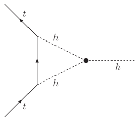
Fig. 2: Correction to the $ht\bar{t}$ coupling in the low energy effective theory below $\Lambda$. The bullet represents a local operator that includes CFT contributions to the 3-point function as well.

3.3 Phenomenology

We now turn to the phenomenology of this class of models. One important question in these models is the size of precision electroweak corrections. The effective operator that contributes to $S$ is obtained from the effective lagrangian Eq. (3.15):

$$\Delta\mathcal{L}_{\rm eff}\sim\frac{\epsilon g_{1}g_{2}}{\Lambda^{2}}h^{\dagger}W^{\mu\nu}hB_{\mu\nu}\sim\frac{g_{1}g_{2}}{16\pi^{2}}W^{\mu\nu}_{3}B_{\mu\nu}+\cdots.$$ (3.25)

This gives a contribution to $S$ with NDA strength, $S\sim 1/\pi$, i.e. similar to small-$N$ technicolor. The $T$ parameter requires breaking of custodial symmetry, and therefore requires an additional hypercharge loop. The effective coupling that gives rise to $T$ is therefore

$$\Delta\mathcal{L}_{\rm eff}\sim\frac{g_{1}^{2}}{16\pi^{2}}\frac{16\pi^{2}\epsilon^{2}}{\Lambda^{2}}|h^{\dagger}D_{\mu}h|^{2}\sim\frac{\epsilon g_{1}^{2}m_{Z}^{2}}{16\pi^{2}}Z_{\mu}^{2}+\cdots,$$ (3.26)

where $Z_{\mu}$ is the $Z$ boson field. This gives a contribution to $T$ that is parametrically smaller than the NDA value:

$$T\sim\frac{\epsilon}{4\pi}\sim\epsilon\,T_{\rm NDA}.$$ (3.27)

Taken at face value, this is not so great for precision electroweak fits, since the best fit for nonzero electroweak corrections has both $S$ and $T$ positive and comparable. However, given the uncertainties in these estimates these theories are still viable.

The phenomenology at high energy colliders depends on the structure of strong resonances at the TeV scale. We cannot make any rigorous prediction about these resonances other than the fact that they must exist to unitarize WW scattering (the ‘no lose theorem’). In the case where the small dimension of the electroweak order parameter is due to a moderately small parameter in the fundamental theory, we argued above that there will be a prominent scalar resonance below the TeV scale whose couplings to gauge bosons and the top quark are parametrically close to the standard-model values. The deviation from the standard-model value for the coupling to the top quark is quite small, between $1\%$ and $10\%$, while the deviation from the standard model value for the $\phi WW$ coupling is of order $\epsilon$, which is expected to be at least $10\%$. The possibility of studying a ‘non-standard’ heavy Higgs-like scalar at the LHC has been discussed by a number of authors [24]. The discovery of such a particle and the measurement of deviations from the standard-model predictions for its couplings may well be the first indication of strong conformal dynamics as the origin of electroweak symmetry breaking.

4 Conclusions

We have described a new paradigm for dynamical electroweak symmetry breaking in which the electroweak symmetry breaking sector is a conformal field theory (CFT) above the TeV scale. Conformal symmetry and electroweak symmetry are broken at the TeV scale, triggered by an asymptotically-free gauge group or a slightly relevant operator becoming strong, or by a relevant operator with a coefficient made small naturally by symmetries. Any of these mechanisms stabilizes the weak scale against quantum corrections and gives a solution of the hierarchy problem.

The flavor problem of dynamical electroweak symmetry breaking is solved if the dimension of the CFT operator that acts as the order parameter for electroweak symmetry breaking has a dimension $d$ close to 1, the dimension of an elementary Higgs scalar field. For $d=1+\epsilon$, the scale where the top quark Yukawa coupling becomes strong is raised to $\Lambda_{\rm EW}(\Lambda_{\rm EW}/m_{t})^{1/\epsilon}$, where $\Lambda_{\rm EW}\sim 2\mathrm{~{}TeV}$. For $\epsilon\sim 1/{\rm few}$, this is large enough to effectively decouple flavor.

Finding a CFT with the required properties is highly nontrivial. Weakly coupled CFT’s can certainly have operators with dimension near 1 in the form of an elementary scalar Higgs field $h$, but this clearly does not solve the hierarchy problem because of the existence of the relevant operator $h^{\dagger}h$ with dimension near 2. What is required is a strongly-coupled CFT with a scalar operator $\mathcal{O}$ with dimension $d=1+\epsilon$, where strong CFT dynamics renders the operator $\mathcal{O}^{\dagger}\mathcal{O}$ irrelevant by giving it a large anomalous dimension. We have shown, however, that strong CFT’s with large $N$, including those obtained from the AdS/CFT correspondence, have the property that the dimension of $\mathcal{O}^{\dagger}\mathcal{O}$ is close to $2d$, and are therefore fine-tuned for $d<2$.

We are therefore led to consider strongly-coupled, small-$N$ CFT’s. These theories also naturally have small electroweak precision corrections, addressing another strong constraint on models of dynamical electroweak symmetry breaking. The difficulty is that there are no reliable theoretical tools for studying such theories, and in fact no explicit examples are known. In the case where the smallness of $\epsilon$ is due to a small parameter in the fundamental theory, we argued that there will be a prominent scalar resonance with couplings to gauge bosons and the top quark that are comparable to that of a heavy standard-model Higgs, but with $O(\epsilon)$ deviations that can be measured at LHC. We believe that this gives strong motivation to experimental studies of a heavy Higgs-like particle, and look forward to a decisive test of these ideas.

Appendix A: Composite Fermions

In this appendix, we consider the possibility that fermion masses are generated by mixing with fermionic operators of the CFT. That is, we suppose that the CFT contains operators with quantum numbers conjugate to the standard model fermion fields, and we include interaction terms

$$\delta\mathcal{L}=z_{Q}Q\mathcal{Q}^{\rm c}+z_{u}u^{\rm c}\mathcal{U}+z_{d}d^{\rm c}\mathcal{D}+z_{L}L\mathcal{L}^{\rm c}+z_{e}e^{\rm c}\mathcal{E},$$ (A.1)

where $Q,\ldots,e^{\rm c}$ are standard model fermions, and $\mathcal{Q}^{\rm c},\ldots,\mathcal{E}$ are fermionic CFT operators. The unitarity limit on the dimension of the CFT operators is $d=\frac{3}{2}$, the dimension of a free fermion, so the couplings $z_{Q},\ldots,z_{e}$ can be marginal or even relevant without approaching the unitarity limit for CFT operators. This means that the flavor scale where these operators are generated can be decoupled completely, just as in the standard model. We will show that this mechanism generally require a mild $\sim 10$% tuning to accomodate constraints on $Z\to b\bar{b}$ and the $T$ parameter together with the heavy top mass.

This mechanism for generating fermion masses was first considered in the context of technicolor theories in Ref. [16]. It has been revived recently in the context of RS theories, where it corresponds to putting standard model fermions in the bulk [15]. We consider this framework here using our CFT language, which makes it clear that our analysis is model-independent.

In Eq. (A.1), the couplings $z_{Q},\ldots,z_{e}$ are $3\times 3$ matrices in flavor space. These $z$’s act as spurions that violate the $SU(3)^{5}$ flavor symmetry that is otherwise present, and their transformation properties under the flavor symmetry determine the structure of flavor violation in this model. We will normalize the CFT operators $\mathcal{Q}^{\rm c},\ldots,\mathcal{E}$ so that $z\sim 1$ corresponds to strong coupling at the scale of conformal and electroweak symmetry breaking $\Lambda$. If the conformal and electroweak symmetry breaking is strong with no large or small parameters, NDA tells us that the quark mass matrices are

$$m_{u}=c\Lambda z_{Q}^{\dagger}z_{u},\qquad m_{d}=c\Lambda z_{Q}^{\dagger}z_{d},$$ (A.2)

where $c\sim 1$. To get the top quark mass, we must therefore have

$$(z_{Q}^{\dagger}z_{u})_{33}\sim\frac{m_{t}}{\Lambda}\sim\frac{1}{10}.$$ (A.3)

Because the $z$’s violate flavor and custodial symmetry, they give rise to corrections to the $\rho$ parameter and the $Z\to b\bar{b}$ vertex. Note that the leading corrections to the $\rho$ parameter do not involve internal gauge bosons, so we can ignore the custodial symmetry breaking from $U(1)_{Y}$. In this limit the standard model and the CFT each have a separate $SU(2)_{L}\times SU(2)_{R}$ symmetry, which are broken to diagonal subgroups by $z_{Q}$ and $z_{u,d}$. Specifically, the $z$’s transform like

$$z_{L}&\longrightarrow L_{\rm SM}\,z_{L}L_{\rm CFT}^{\dagger}\\ z_{R}\longrightarrow R_{\rm SM}\,z_{R}R_{\rm CFT}^{\dagger},$$

where $z_{L}\equiv z_{Q}$ and $z_{R}\equiv{\rm diag}(z_{d},\,z_{u})$. Electroweak symmetry is broken with NDA strength in the strong sector in the pattern $[SU(2)_{L}\times SU(2)_{R}]_{\rm CFT}\to SU(2)_{\rm cust,CFT}$, so custodial symmetry breaking in the standard model sector depends on the spurion $z_{u}z_{u}^{\dagger}-z_{d}z_{d}^{\dagger}$. This spurion has $\Delta I_{\rm cust,SM}=1$, while a custodial symmetry violating contribution to the $Z$ mass has $\Delta I_{\rm cust,SM}=2$. Therefore

$$\Delta M_{Z}^{2}\sim\frac{g^{2}\Lambda^{2}}{16\pi^{2}}\mathop{\rm tr}(z_{u}z_{u}^{\dagger}-z_{d}z_{d}^{\dagger})^{2}\sim\frac{g^{2}\Lambda^{2}}{16\pi^{2}}\mathop{\rm tr}(z_{u}z_{u}^{\dagger})^{2}$$ (A.4)

In order to satisfy the constraint on the $\rho$ (or $T$) parameter, we require

$$\mathop{\rm tr}(z_{u}z_{u}^{\dagger})^{2}\mathrel{{\mathrel{\raise 1.29167pt\hbox{$<$\kern-7.5pt\lower 4.30554pt\hbox{$\sim$}}}}}\frac{1}{100}.$$ (A.5)

On the other hand, the correction to the $Z\to b_{L}\bar{b}_{L}$ vertex is

$$\Delta g_{Z\to b\bar{b}}\sim 4\pi\frac{g}{4\pi}(z_{Q}^{\dagger}z_{Q})_{33}.$$ (A.6)

Satisfying the experimental constraint requires

$$(z_{Q}^{\dagger}z_{Q})_{33}\mathrel{{\mathrel{\raise 1.29167pt\hbox{$<$\kern-7.5pt\lower 4.30554pt\hbox{$\sim$}}}}}\frac{1}{100}.$$ (A.7)

We see that generically there is a tension in satisfying all three constraints: the $\rho$ parameter constraint (A.5), the $Z\to b\bar{b}$ constraint (A.7) and the top mass condition (A.3). For example, with $(z_{Q})_{33}\sim 1$, Eq. (A.3) forces $(z_{u})_{33}\sim\frac{1}{10}$, which makes the $\rho$ constraint completely safe while requiring an additional contribution to the $Z\to b\bar{b}$ coupling that cancels the non-standard one to $1\%$ accuracy. With $z_{u}\sim 1$, the $Z\to b\bar{b}$ constraint is just on the edge while the $\rho$ constraint needs $1\%$ tuning. However, we can ‘compromise’ and choose $(z_{Q})_{33}\sim(z_{u})_{33}\sim\frac{1}{3}$, which puts us just on the edge of the $\rho$ constraint, while we must find additional contributions to $Z\to b\bar{b}$ that cancel the unwanted CFT contribution to $10\%$ accuracy. Therefore, in this part of the parameter space, this framework is viable with mild tuning.

References

- [1] L. Susskind, Phys. Rev. D 20, 2619 (1979); S. Weinberg, Phys. Rev. D 13, 974 (1976); S. Weinberg, Phys. Rev. D 19, 1277 (1979).
- [2] B. Holdom and J. Terning, Phys. Lett. B 247, 88 (1990); M. Golden and L. Randall, Nucl. Phys. B 361, 3 (1991); M. E. Peskin and T. Takeuchi, Phys. Rev. D 46, 381 (1992).
- [3] S. Eidelman et al. [Particle Data Group Collaboration], Phys. Lett. B 592, 1 (2004).
- [4] B. Holdom, Phys. Lett. B 150, 301 (1985); T. Akiba and T. Yanagida, Phys. Lett. B 169, 432 (1986); T. W. Appelquist, D. Karabali and L. C. R. Wijewardhana, Phys. Rev. Lett. 57, 957 (1986); K. Yamawaki, M. Bando and K. i. Matumoto, Phys. Rev. Lett. 56, 1335 (1986); T. Appelquist and L. C. R. Wijewardhana, Phys. Rev. D 35, 774 (1987); Phys. Rev. D 36, 568 (1987).
- [5] L. Randall and R. Sundrum, Phys. Rev. Lett. 83, 3370 (1999) [arXiv:hep-ph/9905221].
- [6] H. Davoudiasl, J. L. Hewett and T. G. Rizzo, Phys. Lett. B 473, 43 (2000) [arXiv:hep-ph/9911262]; A. Pomarol, Phys. Lett. B 486, 153 (2000) [arXiv:hep-ph/9911294].
- [7] J. M. Maldacena, Adv. Theor. Math. Phys. 2, 231 (1998) [Int. J. Theor. Phys. 38, 1113 (1999)] [arXiv:hep-th/9711200]; E. Witten, Adv. Theor. Math. Phys. 2, 253 (1998) [arXiv:hep-th/9802150]; H. Verlinde, Nucl. Phys. B 580, 264 (2000) [arXiv:hep-th/9906182]; J. Maldacena, unpublished remarks; E. Witten, 1999 ITP Santa Barbara conference ‘New Dimensions in Field Theory and String Theory,’, http://www.itp.ucsb.edu/online/susy c99/discussion; E. Verlinde and H. Verlinde, JHEP 0005, 034 (2000) [arXiv:hep-th/9912018]; N. Arkani-Hamed, M. Porrati and L. Randall, JHEP 0108, 017 (2001) [arXiv:hep-th/0012148]; R. Rattazzi and A. Zaffaroni, JHEP 0104, 021 (2001) [arXiv:hep-th/0012248].
- [8] S. Dimopoulos and L. Susskind, Nucl. Phys. B 155, 237 (1979); E. Eichten and K. D. Lane, Phys. Lett. B 90, 125 (1980).
- [9] A. G. Cohen and H. Georgi, Nucl. Phys. B 314, 7 (1989).
- [10] T. Appelquist, M. Einhorn, T. Takeuchi and L. C. R. Wijewardhana, Phys. Lett. B 220, 223 (1989); V. A. Miransky and K. Yamawaki, Mod. Phys. Lett. A 4, 129 (1989); K. Matumoto, Prog. Theor. Phys. 81, 277 (1989); V. A. Miransky, M. Tanabashi and K. Yamawaki, Phys. Lett. B 221, 177 (1989); Mod. Phys. Lett. A 4, 1043 (1989).
- [11] T. Appelquist, J. Terning and L. C. R. Wijewardhana, Phys. Rev. Lett. 79, 2767 (1997) [arXiv:hep-ph/9706238].
- [12] G. Mack, Commun. Math. Phys. 55, 1 (1977); S. Minwalla, Adv. Theor. Math. Phys. 2, 781 (1998) [arXiv:hep-th/9712074].
- [13] O. Aharony, A. Fayyazuddin and J. M. Maldacena, JHEP 9807, 013 (1998) [arXiv:hep-th/9806159].
- [14] M. J. Strassler, arXiv:hep-th/0309122.
- [15] Y. Grossman and M. Neubert, Phys. Lett. B 474, 361 (2000) [arXiv:hep-ph/9912408]; T. Gherghetta and A. Pomarol, Nucl. Phys. B 586, 141 (2000) [arXiv:hep-ph/0003129]; S. J. Huber and Q. Shafi, Phys. Rev. D 63, 045010 (2001) [arXiv:hep-ph/0005286]; Phys. Lett. B 498, 256 (2001) [arXiv:hep-ph/0010195].
- [16] D. B. Kaplan, Nucl. Phys. B 365, 259 (1991).
- [17] K. Agashe, A. Delgado, M. J. May and R. Sundrum, JHEP 0308, 050 (2003) [arXiv:hep-ph/0308036].
- [18] A. de Gouvea, A. Friedland and H. Murayama, Phys. Rev. D 59, 105008 (1999) [arXiv:hep-th/9810020].
- [19] T. Banks and A. Zaks, Nucl. Phys. B 196, 189 (1982).
- [20] T. Appelquist, A. Ratnaweera, J. Terning and L. C. R. Wijewardhana, Phys. Rev. D 58, 105017 (1998) [arXiv:hep-ph/9806472].
- [21] P. Breitenlohner and D. Z. Freedman, Annals Phys. 144, 249 (1982).
- [22] I. R. Klebanov and E. Witten, Nucl. Phys. B 556, 89 (1999) [arXiv:hep-th/9905104].
- [23] C. Csaki, J. Erlich and J. Terning, Phys. Rev. D 66, 064021 (2002) [arXiv:hep-ph/0203034]; K. Agashe, A. Delgado, M. J. May and R. Sundrum, JHEP 0308, 050 (2003) [arXiv:hep-ph/0308036]; G. Cacciapaglia, C. Csaki, C. Grojean and J. Terning, [arXiv:hep-ph/0401160].
- [24] J. Bagger, S. Dawson and G. Valencia, Nucl. Phys. B 399, 364 (1993) [arXiv:hep-ph/9204211]; J. Bagger, V. D. Barger, K. Cheung, J. F. Gunion, T. Han, G. A. Ladinsky, R. Rosenfeld, C. P. Yuan, Phys. Rev. D 52, 3878 (1995) [arXiv:hep-ph/9504426]; K. Iordanidis and D. Zeppenfeld, Phys. Rev. D 57, 3072 (1998) [arXiv:hep-ph/9709506]; H. J. He, Y. P. Kuang, C. P. Yuan and B. Zhang, Phys. Lett. B 554, 64 (2003) [arXiv:hep-ph/0211229]; B. Zhang, Y. P. Kuang, H. J. He and C. P. Yuan, Phys. Rev. D 67, 114024 (2003) [arXiv:hep-ph/0303048].