Two–Loop Bethe Logarithms for Higher Excited $S$ Levels

Abstract

Processes mediated by two virtual low-energy photons contribute quite significantly to the energy of hydrogenic $S$ states. The corresponding level shift is of the order of $(\alpha/\pi)^{2}\,(Z\alpha)^{6}\,m_{\rm e}\,c^{2}$ and may be ascribed to a two-loop generalization of the Bethe logarithm. For $1S$ and $2S$ states, the correction has recently been evaluated by Pachucki and Jentschura [Phys. Rev. Lett. 91, 113005 (2003)]. Here, we generalize the approach to higher excited $S$ states, which in contrast to the $1S$ and $2S$ states can decay to $P$ states via the electric-dipole ($E1$) channel. The more complex structure of the excited-state wave functions and the necessity to subtract $P$-state poles lead to additional calculational problems. In addition to the calculation of the excited-state two-loop energy shift, we investigate the ambiguity in the energy level definition due to squared decay rates.

I INTRODUCTION

Both the experimental and the theoretical study of radiative corrections to bound-state energies have been the subject of a continued endeavor over the last decades (for topical reviews see Sapirstein and Yennie (1990); Mohr et al. (1998); Eides et al. (2001); Shabaev (2002)). Simple atomic systems like atomic hydrogen, and heliumlike or lithiumlike systems, provide a testbed for our understanding of the fundamental interactions of light and matter, including the intricacies of the renormalization procedure and the complexities of the bound-state formalism. One of the historically most problematic corrections for bound states in hydrogenlike systems is the two-loop self-energy (2LSE) effect (relevant Feynman diagrams in Fig. 1), and this correction will be the subject of the current paper.

Figure 1: Two-photon processes may be interpreted in terms of Feynman diagrams. The double line denotes the bound-electron propagator. In the figure, we display the crossed-loop (A), the rainbow (B), and the loop-after-loop (C) diagram.

Regarding self-energy calculations, two different approaches have been developed for hydrogenlike systems: (i) the semianalytic approach, which is the so-called $Z\alpha$ expansion and in which the radiative corrections are expressed as a semianalytic series expansion in the quantities $Z\alpha$ and $\ln[(Z\alpha)^{-2}]$, and (ii) the numerical approach, which avoids this expansion and leads to excellent accuracy for systems with a high nuclear charge number. Over the last couple of years, a number of calculations have been reported that profit from recently developed numerical algorithms and an improved physical understanding of the problem at hand. These have led to numerical results even at low nuclear charge number Jentschura et al. (1999, 2001); Yerokhin et al. (2002).

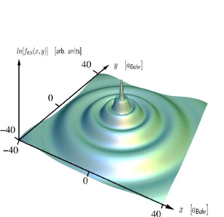
Figure 2: (color online). Hydrogenic $S$ levels have the same (radial) symmetry properties as the ground state. The wave function $\psi(r)$ of an $S$ level therefore depends only on the radial coordinate $r\equiv\sqrt{x^{2}+y^{2}+z^{2}}$. The function $f_{\rm 6S}(x,y)\equiv\int^{\infty}_{-\infty}{\rm d}z\,\left|\psi_{\rm 6S}(x,y,z)\right|^{2}$ is positive definite and constitutes effectively an integrated projection of the $6S$ electron probability density onto the $x$-$y$ plane. Indeed, we plot here the natural logarithm of this function, which is $\ln[f_{\rm 6S}(x,y)]$, as a function of $x\in[-40\,a_{\rm Bohr},40\,a_{\rm Bohr}]$ and $y\in[-40\,a_{\rm Bohr},40\,a_{\rm Bohr}]$. Here, $a_{\rm Bohr}$ denotes the Bohr radius $a_{\rm Bohr}=\hbar/(\alpha mc)=0.529\,177\,2108(18)\times 10^{-10}\,{\rm m}$ MoT .

Within approach (i), a number of calculations have recently been reported which rely on a separation of the energy scale(s) of the virtual photon(s) into high- and low-energy domains (see, e.g., (Berestetskii et al., 1982, Chap. 123), (Itzykson and Zuber, 1980, Chap. 7) and Pachucki (1993a)). This has recently been generalized to two-loop corrections Pachucki (2001); Jentschura and Pachucki (2002). Also, there have been attempts to enhance our understanding of logarithmic corrections in higher orders of the $Z\alpha$ expansion by renormalization-group techniques Manohar and Stewart (2000); Pineda (2002).

In the current paper, we discuss the evaluation of a specific two-loop correction, which can quite naturally be referred to as the two-loop generalization of the Bethe logarithm, for higher excited $S$ states (see also Fig. 2). The calculation is carried out for the dominant nonlogarithmic contribution to the two-loop self-energy shift of order $\alpha^{2}\,(Z\alpha)^{6}\,m\,c^{2}$, where $m\,c^{2}$ is the rest energy of the electron ($m$ is the rest mass), $\alpha$ is the fine-structure constant, and $Z$ is the nuclear charge number.

The two-loop Bethe logarithm is formally of the same order of magnitude [$\alpha^{2}\,(Z\alpha)^{6}\,m\,c^{2}$] as a specific set of two-loop corrections which are mediated by squared decay rates and whose physical interpretation has been shown to be limited by the predictive power of the Gell–Mann–Low theorem on which bound-state calculations are usually based Jentschura et al. (2002a). For excited $nS$ states ($n\geq 3$), the problematic squared decay rates lead to an ambiguity which we assign to the two-loop Bethe logarithm as a further theoretical source of uncertainty. Beyond the order of $\alpha^{2}\,(Z\alpha)^{6}\,m\,c^{2}$, the definition of an atomic energy level becomes ambiguous, and the evaluation of radiative corrections to energy levels has to be augmented by a more complete theory of the line shape Low (1952); Labzowsky et al. (2001); Jentschura and Mohr (2002); Jentschura et al. (2002a, b); Labzowsky et al. (2002a, b), with the $1S$ state being the only true asymptotic state and therefore—in a strict sense—the only valid in- and out-state in the calculation of $S$-matrix type amplitudes Jentschura et al. (2002a). Further interesting thoughts on questions related to line shape profiles can be found in Mohr (1978); Hillery and Mohr (1980). It had also been pointed out in Sec. VI of Jentschura et al. (1997) that the asymmetry of the natural line shape has to be considered at the order $\alpha^{8}$.

It is tempting to ask how one may intuitively understand the slow convergence of the $Z\alpha$ expansion of the two-loop energy shift. As pointed out in Eides et al. (2001), terms of different order in the $Z\alpha$ expansion have rather distinct physical origins. In the order $\alpha^{2}\,(Z\alpha)^{4}\,m\,c^{2}$, there are two corrections, both arising from hard (high-energy) virtual photons. These correspond, respectively, to the infrared convergent slope of the two-loop electron Dirac form factor and to a two-loop anomalous magnetic moment correction. The term of order $\alpha^{2}\,(Z\alpha)^{5}\,m\,c^{2}$ may also be computed without any consideration of low-energy virtual quanta Pachucki (1993a, 1994); Eides et al. (1994); Eides and Shelyuto (1995); Eides et al. (2001). The terms of order $\alpha^{2}\,(Z\alpha)^{6}\,m\,c^{2}$ are not the leading terms arising from the two-loop self-energy shifts. Logarithmic correction terms of order $\alpha^{2}\,(Z\alpha)^{6}\,\ln^{i}[(Z\alpha)^{-2}]\,m\,c^{2}$ ($i=1,2,3$) have been considered in Karshenboim (1996); Pachucki (2001). It is only at the order of $\alpha^{2}\,(Z\alpha)^{6}\,m\,c^{2}$ that the low-energy virtual photons begin to contribute to the hydrogenic energy shift(s) of $S$ states. They do so quite significantly, enhanced by the triple logarithm ($i=3$) and a surprisingly large coefficient of the single logarithm ($i=1$), as shown in Pachucki (2001). It is therefore evident that we need to gain an understanding of all logarithmic and nonlogarithmic terms ($i=0,1,2,3$) of order $\alpha^{2}\,(Z\alpha)^{6}\,\ln^{i}[(Z\alpha)^{-2}]\,m\,c^{2}$ before any reliable prediction for the two-loop bound-state correction can be made even at low nuclear charge number.

An interesting observation can be made based on the fact that the imaginary part of the (nonrelativistic) one-loop self-energy gives the leading-order contribution to the $E1$ one-photon decay width of excited states Barbieri and Sucher (1978). Analogously, it is precisely the imaginary part of the nonrelativistic two-loop self-energy which corresponds to the two-photon decay rate of the $2S$ state. The $2S$ two-photon decay rate is of the order of $\alpha^{2}\,(Z\alpha)^{6}\,m\,c^{2}$ (see, e.g., Shapiro and Breit (1959); Klarsfeld (1969); Cresser et al. (1986); Florescu et al. (1988)). From a nonrelativistic point of view, the scaling $\alpha^{2}\,(Z\alpha)^{6}\,m\,c^{2}$ can be seen as some kind of “natural” order for the two-loop effect. It is the first order in which logarithms of $Z\alpha$ appear and the first order in which a matching of low- and high-energy contributions is required. This is also reflected in the properties of the two-photon decay.

This article is organized as follows. In Sec. II, we review the status of known two-loop self-energy corrections. The formulation of the problem in nonrelativistic quantum electrodynamics (NRQED) and calculation is discussed in Sec. III. Squared decay rates are the subject of Sec. IV, and further contributions to the self-energy in the order of $\alpha^{2}\,(Z\alpha)^{6}\,m\,c^{2}$ are discussed in Sec. V. Finally, conclusions are drawn in Sec. VI.

II KNOWN TWO–LOOP SELF–ENERGY COEFFICIENTS

We work in natural units ($\hbar=c=\epsilon_{0}=1$), as is customary in QED bound-state calculations. The (real part of the) level shift of a hydrogenic state due to the two-loop self-energy reads

$$\Delta E^{\rm(2L)}_{\mathrm{SE}} = \left(\frac{\alpha}{\pi}\right)^{2}\,\frac{(Z\alpha)^{4}\,m_{\rm e}}{n^{3}}\,H(Z\alpha)\,.$$ (1)

For the two-loop self-energy (2LSE) diagrams (see Fig. 1), the first terms of the semianalytic expansion in powers of $Z\alpha$ and $\ln[(Z\alpha)^{-2}]$ read

$$H(Z\alpha)=B^{\rm(2LSE)}_{40}+(Z\alpha)\,B^{\rm(2LSE)}_{50}$$ (2)

$$+(Z\alpha)^{2}\,\left\{B^{\rm(2LSE)}_{63}\,\ln^{3}(Z\alpha)^{-2}+B^{\rm(2LSE)}_{62}\,\ln^{2}(Z\alpha)^{-2}\right.$$

$$\left.+B^{\rm(2LSE)}_{61}\,\ln(Z\alpha)^{-2}+B^{\rm(2LSE)}_{60}\right\}\,.$$

The function $H(Z\alpha)$ is dimensionless. We ignore unknown higher-order terms in the $Z\alpha$ expansion and focus on a specific numerically large contribution to $B^{\rm(2LSE)}_{60}$ given by the two-loop Bethe logarithm. We also keep the upper index (2LSE) in order to distinguish the two-loop self-energy contributions to the analytic coefficients from the self-energy vacuum-polarization (SEVP) effects Pachucki (2001); Jentschura (2003a) and the vacuum-polarization insertion into the virtual photon line in the one-loop self-energy (SVPE). By contrast, the sum of these effects carries no upper index, according to a convention adopted previously in Pachucki (2001); Jentschura (2003a). It has been mentioned earlier that $B_{40}$ and $B_{50}$ are purely relativistic effects mediated by hard virtual photons. The coefficient $B_{40}$ in Eq. (2) involves a Dirac and a Pauli form factor correction and reads Two

$$B^{\rm(2LSE)}_{40}(nS)=-\frac{163}{72}-\frac{85}{36}\,\zeta(2)+9\,\ln(2)\,\zeta(2)-\frac{9}{4}\,\zeta(3)\,;$$ (3)

the numerical value is $1.409\,244$. The first relativistic correction $B^{\rm(2LSE)}_{50}(nS)$ is known to have a rather large value Pachucki (1994),

$$B^{\rm(2LSE)}_{50}(nS)=-24.2668(31)\,.$$ (4)

The triple logarithm in the sixth order of $Z\alpha$ reads,

$$B_{63}(nS)=B^{\rm(2LSE)}_{63}(nS)=-\frac{8}{27}\,.$$ (5)

It has meanwhile been clarified Yerokhin (2000, 2001); Jentschura and Nandori (2002); Yerokhin et al. (2003) that the total value of this coefficient is the result of subtle cancellations among the different diagrams displayed in Fig. 1. The double logarithm for $nS$ is given by

$$B^{\rm(2LSE)}_{62}(1S) = \frac{16}{27}-\frac{16}{9}\,\ln(2)=-0.639\,669\,,$$ (6)

$$B^{\rm(2LSE)}_{62}(nS) = B^{\rm(2LSE)}_{62}(1S)$$ (7)

$$\!\!\!\!\!\!\!\!\!\!\!\!\!\!\!\!\!\!\!\!\!\!\!\!\!\!\!\!\!\!\!\!+\frac{16}{9}\left(\frac{3}{4}+\frac{1}{4n^{2}}-\frac{1}{n}-\ln(n)\!+\!\Psi(n)+C\right),$$

where $\Psi$ denotes the logarithmic derivative of the gamma function, and $C=0.577216\dots$ is Euler’s constant.

The result for $B_{61}$, restricted to the two-loop diagrams in Fig. 1, reads Pachucki (2001); Jentschura (2003a)

$$B^{\rm(2LSE)}_{61}(1S) = \frac{5\,221}{1\,296}+\frac{875}{72}\,\zeta(2)+\frac{9}{2}\,\,\zeta(2)\,\ln 2$$ (8)

$$-\frac{9}{8}\,\zeta(3)-\frac{152}{27}\,\ln 2+\frac{40}{9}\,\ln^{2}2$$

$$+\frac{4}{3}\,N(1S)$$

$$= 49.838\,317\,,$$

$$B^{\rm(2LSE)}_{61}(nS) = B^{\rm(2LSE)}_{61}(1S)+\frac{4}{3}\,\left[N(nS)-N(1S)\right]$$ (9)

$$+\!\left(\frac{80}{27}-\frac{32}{9}\,\ln 2\right)\,\left(\frac{3}{4}+\frac{1}{4n^{2}}\right.$$

$$\left.-\frac{1}{n}-\ln(n)\!+\!\Psi(n)\!+\!C\right)\,.$$

We correct here a calculational error in Eq. (7a) of Ref. Jentschura (2003a) where a result of $49.731651$ had been given for $B^{\rm(2LSE)}_{61}(1S)$. However, even with this correction, the result for $B^{\rm(2LSE)}_{61}(1S)$ given in Eq. (8) is incomplete because it lacks contributions from two-Coulomb-vertex diagrams. These diagrams give rise to an effective interaction proportional to $\bm{E}^{2}$ in the NRQED Hamiltonian and will be discussed in Pachucki et al. (a). The additional contribution to $B^{\rm(2LSE)}_{61}(1S)$ does not affect the $n$-dependence of this coefficient as indicated in Eq. (9), nor does it affect the calculation of the two-loop Bethe logarithms presented in this article.

Numerical values of $N(nS)$ are given in (Jentschura, 2003b, Eq. (12)) for $n=1,\dots,8$:

$$N(1S) = 17.855\,672(1)\,,$$ (10a)

$$N(2S) = 12.032\,209(1)\,,$$ (10b)

$$N({3S}) = 10.449\,810(1)\,,$$ (10c)

$$N(4S) = 9.722\,413(1)\,,$$ (10d)

$$N(5S) = 9.304\,114(1)\,,$$ (10e)

$$N(6S) = 9.031\,832(1)\,,$$ (10f)

$$N(7S) = 8.840\,123(1)\,,$$ (10g)

$$N(8S) = 8.697\,639(1)\,.$$ (10h)

III TWO–LOOP PROBLEM IN NRQED

Historically, one of the first two-photon problems to be tackled theoretically in atomic physics has been the two-photon decay of the metastable $2S$ level which was treated in  Göppert (1929); Göppert-Mayer (1931). It is this decay channel which limits the lifetime of the $2S$ hydrogenic state. We have Shapiro and Breit (1959)

$$\tau^{-1}=\Gamma=8.229\,Z^{6}\,{\rm s}^{-1}=1.310\,Z^{6}\,{\rm Hz}\,.$$ (11)

The numerical prefactors of the width is different when expressed in inverse seconds and alternatively in Hz. The following remarks are meant to clarify this situation as well as the entries in Table 2 below. In order to obtain the width in Hz, one should interpret the imaginary part of the self-energy Barbieri and Sucher (1978) as $\Gamma/2$, and do the same conversion as for the real part of the energy, i.e. divide by $h$, not $\hbar$. This gives the width in Hz. The unit Hz corresponds to cycles per second.

In order to obtain the lifetime in inverse seconds, which is radians per second, one has to multiply the previous result by a factor of $2\pi$, a result which may alternatively be obtained by dividing $\Gamma$—i.e. the imaginary part of the energy, by $\hbar$, not $h$. The general paradigm is that in order to evaluate an energy in units of Hz, one should use the relation $E=h\,\nu$, whereas for a conversion of an imaginary part of an energy to the inverse lifetime, one should use $\Gamma=\hbar\,\tau^{-1}$. As calculated in Refs. Shapiro and Breit (1959); Klarsfeld (1969), the width of the metastable $2S$ state in atomic hydrogenlike systems is $8.229\,Z^{6}\,{\rm s}^{-1}$ (inverse seconds). At $Z=1$, this is equivalent to the “famous” value of $1.3\,{\rm Hz}$ which is nowadays most frequently quoted in the literature. The lifetime of a hydrogenic $2S$ level is thus $0.1215\,Z^{-6}\,{\rm s}$. This latter fact has been verified experimentally for ionized helium Prior (1972); Kocher et al. (1972); Hinds et al. (1978).

We now briefly recall the expression for the two-photon decay involving two emitted photons with polarization vectors $\bm{\varepsilon}_{1}$ and $\bm{\varepsilon}_{2}$, in a two-photon transition from an initial state $|\phi_{i}\rangle$ to a final state $|\phi_{f}\rangle$. The two-photon decay width $\Gamma$ is given by [see, for example, Eq. (3) of Ref. Shapiro and Breit (1959)]

$$\Gamma = \frac{4}{27}\,\frac{\alpha^{2}}{\pi}\,\int\limits^{\omega_{\rm max}}_{0}{\rm d}\omega_{1}\,\omega^{3}_{1}\,\omega^{3}_{2}\,$$ (12)

$$\left|\left<\phi_{f}\left|x^{i}\,\frac{1}{H-E+\omega_{2}}\,x^{i}\right|\phi_{i}\right>\right.$$

$$\left.+\left<\phi_{f}\left|x^{i}\,\frac{1}{H-E+\omega_{1}}\,x^{i}\right|\phi_{i}\right>\right|^{2}\,,$$

where $\omega_{2}=\omega_{\rm max}-\omega_{1}$ and $\omega_{\rm max}=E-E^{\prime}$ is the maximum energy that any of the two photons may have. The Einstein summation convention is used throughout this article. Note the identity Bassani et al. (1977); Kobe (1978)

$$\left<\phi_{f}\left|\frac{p^{i}}{m}\,\frac{1}{H-E+\omega_{1}}\,\frac{p^{i}}{m}\right|\phi_{i}\right>$$ (13)

$$+\left<\phi_{f}\left|\frac{p^{i}}{m}\,\frac{1}{H-E+\omega_{2}}\,\frac{p^{i}}{m}\right|\phi_{i}\right>$$

$$= -\omega_{1}\,\omega_{2}\,m^{2}\,\left\{\left<\phi_{f}\left|x^{i}\,\frac{1}{H-E+\omega_{1}}\,x^{i}\right|\phi_{i}\right>\right.$$

$$\left.+\left<\phi_{f}\left|x^{i}\,\frac{1}{H-E+\omega_{2}}\,x^{i}\right|\phi_{i}\right>\right\}\,,$$

which is valid at exact resonance $\omega_{1}+\omega_{2}=E_{i}-E_{f}$. This identity permits a reformulation of the problem in the velocity-gauge as opposed to the length-gauge form.

In a number of cases, the formulation of a quantum electrodynamic bound-state problem may be simplified drastically when employing the concepts of an effective low-energy field theory known as nonrelativistic quantum electrodynamics Caswell and Lepage (1986). The basic idea consists in a correspondence between fully relativistic quantum electrodynamics and effective low-energy couplings between the electron and radiation field, which still lead to ultraviolet divergent expressions. However, the ultraviolet divergences may be matched against effective high-energy operators, which leads to a cancellation of the cut-off parameters. Within the context of the one-loop self-energy problem, a specialized approach has been discussed in Pachucki (1993a); Jentschura and Pachucki (1996); Jentschura et al. (1997); Jentschura . The formulation of the two-loop self-energy problem within the context of nonrelativistic quantum electrodynamics (NRQED) has been discussed in Pachucki (2001). We denote by $p^{j}$ the Cartesian components of the momentum operator $\bm{p}=-{\rm i}\,\bm{\nabla}$. The expression for the two-loop self-energy shift reads Pachucki (2001); rem (a)

$$\Delta E_{\rm NRQED}=-\left(\frac{2\,\alpha}{3\,\pi\,m^{2}}\right)^{2}\,\int_{0}^{\epsilon_{1}}{\rm d}\omega_{1}\,\omega_{1}\,\int_{0}^{\epsilon_{2}}{\rm d}\omega_{2}\,\omega_{2}\,\left\{\left<p^{i}\,\frac{1}{H-E+\omega_{1}}\,p^{j}\,\frac{1}{H-E+\omega_{1}+\omega_{2}}\,p^{i}\,\frac{1}{H-E+\omega_{2}}\,p^{j}\right>\right.$$ (14)

$$+\frac{1}{2}\,\left<p^{i}\,\frac{1}{H-E+\omega_{1}}\,p^{j}\,\frac{1}{H-E+\omega_{1}+\omega_{2}}\,p^{j}\,\frac{1}{H-E+\omega_{1}}\,p^{i}\right>$$

$$+\frac{1}{2}\,\left<p^{i}\,\frac{1}{H-E+\omega_{2}}\,p^{j}\,\frac{1}{H-E+\omega_{1}+\omega_{2}}\,p^{j}\,\frac{1}{H-E+\omega_{2}}\,p^{i}\right>$$

$$+\left<p^{i}\,\frac{1}{H-E+\omega_{1}}\,p^{i}\,\left(\frac{1}{H-E}\right)^{\prime}\,p^{j}\,\frac{1}{H-E+\omega_{2}}\,p^{i}\right>$$

$$-\frac{1}{2}\,\left<p^{i}\,\frac{1}{H-E+\omega_{1}}\,p^{i}\right>\,\left<p^{j}\,\left(\frac{1}{H-E+\omega_{2}}\right)^{2}\,p^{i}\right>-\frac{1}{2}\,\left<p^{i}\,\frac{1}{H-E+\omega_{2}}\,p^{i}\right>\,\left<p^{j}\,\left(\frac{1}{H-E+\omega_{1}}\right)^{2}\,p^{i}\right>$$

$$\left.-m\,\left<p^{i}\,\frac{1}{H-E+\omega_{1}}\,\frac{1}{H-E+\omega_{2}}\,p^{i}\right>-\frac{m}{\omega_{1}+\omega_{2}}\,\left<p^{i}\,\frac{1}{H-E+\omega_{2}}\,p^{i}\right>-\frac{m}{\omega_{1}+\omega_{2}}\,\left<p^{i}\,\frac{1}{H-E+\omega_{1}}\,p^{i}\right>\right\}.$$

All of the matrix elements are evaluated on the reference state $|\phi\rangle$, for which the nonrelativistic Schrödinger wave function is employed. The Schrödinger Hamiltonian is denoted by $H$, and $E=-(Z\alpha)^{2}\,m/(2n^{2})$ is the Schrödinger energy of the reference state ($n$ is the principal quantum number).

Expressions (12) and (13) now follow in a natural way as the imaginary part generated by the sum of the first three terms in curly brackets in Eq. (14). Specifically, the poles are generated upon $\omega_{2}$-integration by the propagator

$$\frac{1}{H-E+\omega_{1}+\omega_{2}}=\sum_{j}\frac{|j\rangle\,\langle j|}{E_{j}-E+\omega_{1}+\omega_{2}}$$ (15)

when $E-E_{j}=\omega_{1}+\omega_{2}$, which is just the energy conservation condition for two-photon decay. Of course, other terms in Eq. (14), not just the first three in curly brackets, may also generate imaginary parts (especially if the reference state is an excited state, and one-photon decay is possible). The corresponding pole terms must be dealt with in a principal-value prescription if we are interested only in the real part of the energy shift. For $P$ states and higher excited $S$ states, the remaining imaginary parts find a natural interpretation as radiative correction to the one-photon decay width Sapirstein et al. (2004).

From here on we scale the photon frequencies $\omega_{1,2}$ by

$$\omega_{k}\to\omega^{\prime}_{k}\equiv\frac{\omega_{k}}{(Z\alpha)^{2}\,m}\,,\quad k=1,2\,.$$ (16a)

This scaling, which is convenient for our numerical calculations, (almost) corresponds to a transition to atomic units [but with $$(Z\alpha)^{2}\,m=1$$ instead of a unit Rydberg constant]. The momentum operator is scaled as

$$\bm{p}\to\bm{p}^{\prime}\equiv\frac{\bm{p}}{Z\alpha\,m}$$ (16b)

and becomes a dimensionless quantity. The Schrödinger Hamiltonian is scaled as

$$H\to H^{\prime}\equiv\frac{H}{(Z\alpha)^{2}\,m}\,.$$ (16c)

The binding energy of the reference state receives a scaling as

$$E\to E^{\prime}\equiv\frac{E}{(Z\alpha)^{2}\,m}=-\frac{1}{2n^{2}}$$ (16d)

and is from now on also a dimensionless quantity ($$n$$ is the principal quantum number). The scaled, dimensionless radial coordinate is obtained as

$$r\to r^{\prime}\equiv Z\alpha\,m\,r\,.$$ (16e)

The scaled Green function

$$G^{\prime}(\omega^{\prime})=\frac{1}{E^{\prime}-H^{\prime}-\omega^{\prime}}$$ (16f)

is also dimensionless. Finally, the quantity

$$G^{\prime}_{\rm red}(0)=\sum_{|j\rangle\neq|\phi\rangle}\frac{|j\rangle\,\langle j|}{E^{\prime}-E^{\prime}_{j}}$$ (16g)

is the reduced Green function where the reference state $|\phi\rangle$ is excluded from the sum over intermediate states. The (scaled dimensionless) Schrödinger Hamiltonian is then given as $H^{\prime}=\bm{p}^{\prime 2}/2-1/r^{\prime}$. Scaled quantities will be used from here on until the end of the current Section III, and we will denote the scaled, dimensionless quantities by primes, for absolute clarity of notation. (Note that in Ref. Pachucki and Jentschura (2003), the corresponding scaled quantities were denoted by the same symbol as the dimensionful quantities.) As indicated in (Pachucki and Jentschura, 2003, Eq. (5)), the expression (14) can be rewritten in terms of the scaled quantities as

$$\Delta E_{\rm NRQED}=\frac{4}{9}\,\left(\frac{\alpha}{\pi}\right)^{2}\,(Z\alpha)^{6}\,m\,\int{\rm d}\omega^{\prime}_{1}\int{\rm d}\omega^{\prime}_{2}\,f(\omega^{\prime}_{1},\omega^{\prime}_{2})\,,$$ (17)

where the (dimensionless) function $f(\omega^{\prime}_{1},\omega^{\prime}_{2})$ is defined as [see also Eq. (14)]

$$f(\omega^{\prime}_{1},\omega^{\prime}_{2})=\omega^{\prime}_{1}\,\omega^{\prime}_{2}\,\left[\left<p^{\prime i}\,G^{\prime}(\omega^{\prime}_{1})\,p^{\prime j}\,G^{\prime}(\omega^{\prime}_{1}+\omega^{\prime}_{2})\,p^{\prime i}\,G^{\prime}(\omega^{\prime}_{2})\,p^{\prime j}\right>+\frac{1}{2}\,\left<p^{\prime i}\,G^{\prime}(\omega^{\prime}_{1})\,p^{\prime j}\,G^{\prime}(\omega^{\prime}_{1}+\omega^{\prime}_{2})\,p^{\prime j}\,G^{\prime}(\omega^{\prime}_{1})\,p^{\prime i}\right>\right.$$

$$+\frac{1}{2}\,\left<p^{\prime i}\,G^{\prime}(\omega^{\prime}_{2})\,p^{\prime j}\,G^{\prime}(\omega^{\prime}_{1}+\omega^{\prime}_{2})\,p^{\prime j}\,G^{\prime}(\omega^{\prime}_{2})\,p^{\prime i}\right>+\left<p^{\prime i}\,G^{\prime}(\omega^{\prime}_{1})\,p^{\prime i}\,G^{\prime}_{\rm red}(0)\,p^{\prime j}\,G^{\prime}(\omega^{\prime}_{2})\,p^{\prime i}\right>$$

$$-\frac{1}{2}\,\left<p^{\prime i}\,G^{\prime}(\omega^{\prime}_{1})\,p^{\prime i}\right>\,\left<p^{\prime j}\,G^{\prime 2}(\omega^{\prime}_{2})\,p^{\prime i}\right>-\frac{1}{2}\,\left<p^{\prime i}\,G^{\prime}(\omega^{\prime}_{2})\,p^{\prime i}\right>\,\left<p^{\prime j}\,G^{\prime 2}(\omega^{\prime}_{1})\,p^{\prime i}\right>$$

$$\left.+\left<p^{\prime i}\,G^{\prime}(\omega^{\prime}_{1})\,G^{\prime}(\omega^{\prime}_{2})\,p^{\prime i}\right>-\frac{1}{\omega^{\prime}_{1}+\omega^{\prime}_{2}}\,\left<p^{\prime i}\,G^{\prime}(\omega^{\prime}_{2})\,p^{\prime i}\right>-\frac{1}{\omega^{\prime}_{1}+\omega^{\prime}_{2}}\,\left<p^{\prime i}\,G^{\prime}(\omega^{\prime}_{1})\,p^{\prime i}\right>\right]\,.$$ (18)

In Pachucki and Jentschura (2003), the corresponding Equation (5) has a typographical error: the term $m\,\left<p^{\prime i}\,G^{\prime}(\omega^{\prime}_{1})\,G^{\prime}(\omega^{\prime}_{2})\,p^{\prime i}\right>$ should have a plus instead of a minus sign (seventh term in the square brackets). In particular, the scaling (16) leads to a disappearance of the powers of $Z\alpha$ when considering the expression $\int{\rm d}\omega^{\prime}_{1}\,\omega^{\prime}_{1}\,\int{\rm d}\omega^{\prime}_{2}\,\omega^{\prime}_{2}\,f(\omega^{\prime}_{1},\omega^{\prime}_{2})$.

First, we fix $\omega^{\prime}_{1}$ and integrate over $\omega^{\prime}_{2}$. The subtraction procedure is as follows. We need to subtract the contribution from the following terms that lead to divergent expressions as $\omega^{\prime}_{2}\to\infty$. We therefore expand $f(\omega^{\prime}_{1},\omega^{\prime}_{2})$ for large $\omega^{\prime}_{2}$ at fixed $\omega^{\prime}_{1}$. The asymptotics read Pachucki and Jentschura (2003)

$$f(\omega^{\prime}_{1},\omega^{\prime}_{2}) = a(\omega^{\prime}_{1})+\frac{b(\omega^{\prime}_{1})}{\omega^{\prime}_{2}}+\dots$$ (19)

where the further terms in the expansion of $f(\omega^{\prime}_{1},\omega^{\prime}_{2})$ for $\omega^{\prime}_{2}\to\infty$ lead to convergent expressions when integrated over $\omega^{\prime}_{2}$ in the region of large $\omega^{\prime}_{2}$. The leading coefficient is

$$a(\omega^{\prime}_{1})=\omega^{\prime}_{1}\,\left<p^{\prime i}\,\frac{H^{\prime}-E^{\prime}}{(H^{\prime}-E^{\prime}+\omega^{\prime}_{1})^{2}}\,p^{\prime i}\right>\,,$$ (20)

and the second reads

$$b(\omega^{\prime}_{1})=\omega^{\prime}_{1}\,\,\delta_{W}\left\{\left<p^{\prime i}\,\frac{1}{E^{\prime}-(H^{\prime}+\omega^{\prime}_{1})}\,p^{\prime i}\right>\right\}\,,$$ (21)

where by $\delta_{W}$ we denote the first-order correction to the quantity in curly brackets obtained via the action of the scaled, dimensionless, local potential

$$W=\frac{\pi\,\delta^{(3)}(\bm{r})}{(Z\alpha)^{3}\,m^{3}}=\pi\,\delta^{(3)}(\bm{r}^{\prime})\,,$$ (22)

i.e., by the replacements [see Eq. (16f)],

$$H^{\prime} \to H^{\prime}+W\,,$$ (23a)

$$|\phi\rangle \to |\phi\rangle+|\delta\phi\rangle\,,$$ (23b)

$$E^{\prime} \to E^{\prime}+\delta E^{\prime}\,.$$ (23c)

Here

$$\delta E^{\prime}=\langle W\rangle\,,\qquad|\delta\phi\rangle=G^{\prime}_{\rm red}(0)\,W|\phi\rangle\,.$$ (24)

The correction (21) has been calculated for excited $S$ states in Ref. Jentschura (2003b).

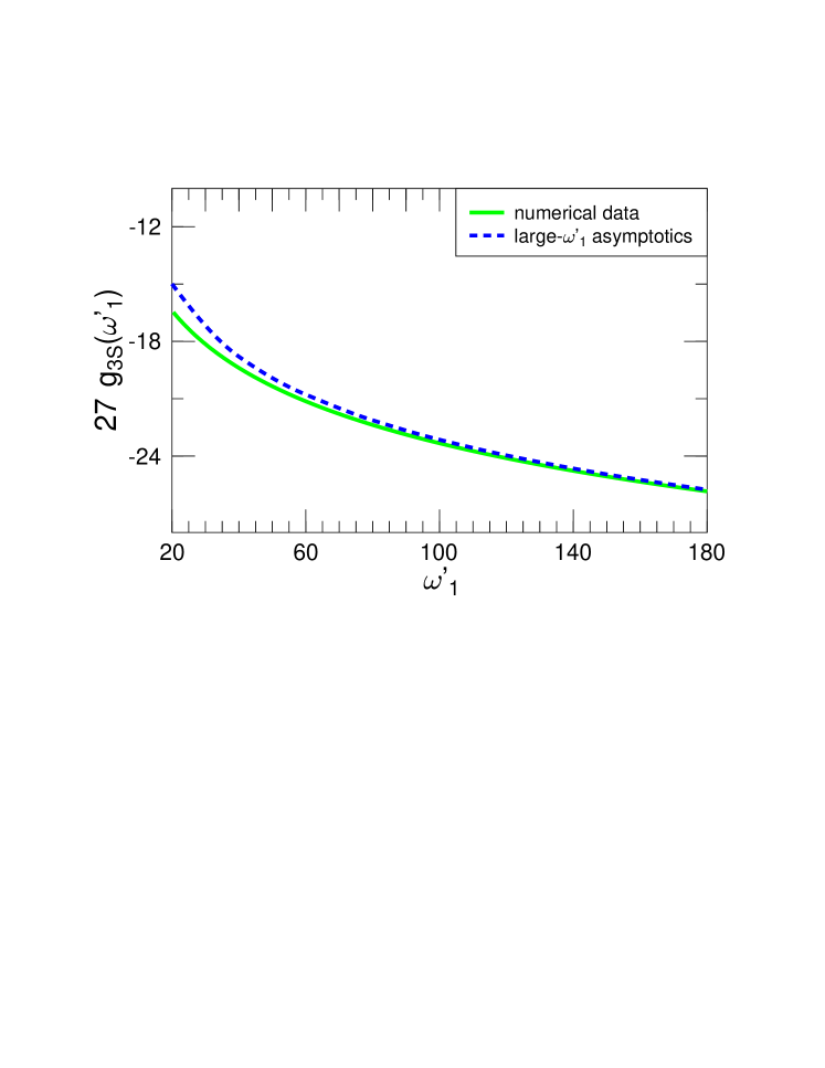
Figure 3: (color online). Plot of the large-$\omega^{\prime}_{1}$ asymptotics of $g$ [see Eq. (29)] against numerical data obtained for $g_{3S}(\omega^{\prime}_{1})$ in the range $\omega^{\prime}_{1}\in[20,180]$. The numerical data are scaled by a factor of $3^{3}=27$. See also Table 1 and Eq. (25a) where $g$ is defined. Dimensionless quantities are displayed in the figure [this statement relates to both the abscissa as well as the ordinate axis, see also Eq. (16)].

We are interested in evaluating the constant term $g(\omega^{\prime}_{1})$ in the integral of $f(\omega^{\prime}_{1},\omega^{\prime}_{2})$ in the range $\omega^{\prime}_{2}\in(0,\Lambda)$ at fixed $\omega^{\prime}_{1}$ for large $\Lambda$:

$$\int_{0}^{\Lambda}{\rm d}\omega^{\prime}_{2}\,f(\omega^{\prime}_{1},\omega^{\prime}_{2})=a(\omega^{\prime}_{1})\,\Lambda+b(\omega^{\prime}_{1})\,\ln\Lambda+g(\omega^{\prime}_{1})\,,$$ (25a)

where we neglect terms that vanish as $$\Lambda\to\infty g(\omega^{\prime}_{1}) \Lambda\to 0$$. This equation provides an implicit definition of as the constant term which results in the limit . The constant term may be evaluated as

$$g(\omega^{\prime}_{1})={\cal I}_{1}+{\cal I}_{2}+{\cal I}_{3}\,,$$ (25b)

where

$${\cal I}_{1} = \int_{0}^{M}{\rm d}\omega^{\prime}_{2}\,f(\omega^{\prime}_{1},\omega^{\prime}_{2})\,,$$ (26a)

$${\cal I}_{2} = \int_{M}^{\infty}{\rm d}\omega^{\prime}_{2}\left[f(\omega^{\prime}_{1},\omega^{\prime}_{2})-a(\omega^{\prime}_{1})-\frac{b(\omega^{\prime}_{1})}{\omega^{\prime}_{2}}\right]\,,$$ (26b)

$${\cal I}_{3} = -a(\omega^{\prime}_{1})\,M-b(\omega^{\prime}_{1})\,\ln M\,,$$ (26c)

with arbitrary $M$ [the result for $g(\omega^{\prime}_{1})$ is independent of $M$]. Sample values of the $g$-function for $nS$ states are given in Table 1. The sign of the ${\cal I}_{3}$-term (cf. (Pachucki and Jentschura, 2003, Eq. (8c))) is determined by the necessity of subtracting the integral of the subtraction term [second term in the integrand of Eq. (26b)], at the lower limit of integration $M$. In both the $\omega^{\prime}_{1}$ as well as the $\omega^{\prime}_{2}$ integrations, there is a further complication due to bound-state poles ($P$ states) which need to be considered for higher excited $nS$ states ($n\geq 3$). In the current section, we completely ignore the imaginary parts and carry out all integrations with a principal-value prescription. Idem est, we use the prescription ($M>a$)

$$\int_{0}^{M}{\rm d}\omega^{\prime}\,\frac{1}{(\omega^{\prime}-a)}\to\ln\left(\frac{M-a}{a}\right)\,.$$ (27)

For double poles, which originate from some of the terms in Eq. (14), the appropriate integration prescription is as follows:

$$\int_{0}^{M}{\rm d}\omega^{\prime}\,\frac{1}{(\omega^{\prime}-a)^{2}}\to\frac{M}{a\,(a-M)}\,.$$ (28)

Even if $M>a$, this prescription leads to a finite result which is real rather than complex. The same result can also be obtained under a symmetric deformation of the integration contour into the complex plane. Analogous integration prescriptions have been used in Jentschura and Pachucki (1996); Jentschura et al. (1997). Double poles normally lead to nonintegrable singularities and give rise to serious concern. It is therefore necessary to ask how these terms originate in the context of the current calculation. To answer this question it is useful to remember that expression (14) is obtained by perturbation theory in powers of the nonrelativistic QED interaction Lagrangian; an expansion in powers of the interaction is, however, not allowed when we are working close to a resonance of the unperturbed atomic Green function—i.e., close to a bound-state pole. The double poles incurred by this expansion find a natural a posteriori treatment by the prescriptions (27) and (28) above. In general, double poles as encountered here and previously in Jentschura and Pachucki (1996); Jentschura et al. (1997) originate whenever we work with (i) excited states which can decay through $E1$ one-photon emission and (ii) propagators are perturbatively expanded near bound-state poles.

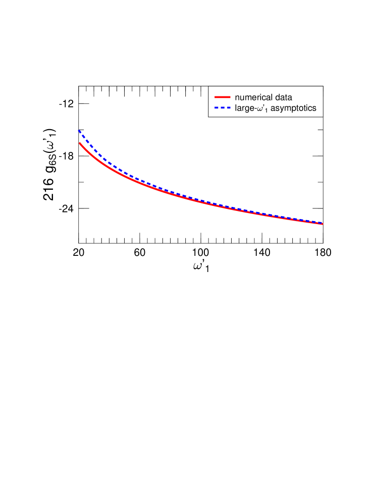
Figure 4: (color online). Large-$\omega^{\prime}_{1}$ asymptotics of $g$ plotted against numerical data for the $6S$ state in the range $\omega^{\prime}_{1}\in[20,180]$. The numerical data are scaled by a factor of $6^{3}=216$. Explicit numerical sample values for $g_{6S}(\omega^{\prime}_{1})$ can also be found in Table 1. The apparent similarity of Figs. 3 and 4 is reflected in the scaled entries in this Table. The difference between the numerical data (solid line) and the asymptotics (dashed line) is negative. The formula for the large-$\omega^{\prime}_{1}$ asymptotics of $g$ is given in Eqs. (29) and (30). The difference between the numerical data and the asymptotics gives rise to a negative contribution to the integral $J_{2}$ defined according to Eq. (33b) and to a negative value for the $B_{60}$-coefficient [see Eq. (52) below]. The scaled, primed quantities plotted along both the abscissa as well as the ordinate axis are dimensionless [see also Eq. (16)].

The leading terms in the asymptotics of $g(\omega^{\prime}_{1})$ for large $\omega^{\prime}_{1}$ read Pachucki and Jentschura (2003)

$$g(\omega^{\prime}_{1}) = \frac{1}{n^{3}}\,\left[A\,\ln\omega^{\prime}_{1}+B+C\,\frac{\ln(\omega^{\prime}_{1})}{\sqrt{\omega^{\prime}_{1}}}+D\,\frac{1}{\sqrt{\omega^{\prime}_{1}}}\right.$$ (29)

$$\left.+E\,\frac{\ln^{2}(\omega^{\prime}_{1})}{\omega^{\prime}_{1}}+F\,\frac{1}{\omega^{\prime}_{1}}\right]+\dots,$$

where

$$A = -4\,,$$ (30a)

$$B = 2\,\left[\ln 2-1-\ln k_{0}(nS)\right]\,,$$ (30b)

$$C = 4\,\sqrt{2}\,,$$ (30c)

$$D = 4\,\sqrt{2}\,\left(2\,(\ln 2-1)-\pi\right)\,,$$ (30d)

$$E = 1\,,$$ (30e)

$$F = 8+\frac{3}{2}\,N(nS)+5\pi^{2}\,.$$ (30f)

The higher-order terms in the large-$\omega^{\prime}_{1}$ expansion, which are ignored in Eq. (29), lead to convergent expressions in the problematic integration region $\omega^{\prime}_{1}\to\infty$. Explicit numerical values for $N(nS)$ are given in Eq. (10). For ${3S}$ and $6S$ states, numerical data for $g$ are compared to the leading asymptotics in Figs. 3 and 4.

The two-loop Bethe logarithm, which is equal to the low-energy contribution $B^{\rm lep}_{60}(nS)$ to the coefficient $B^{\rm(2LSE)}_{60}$ [see Eq. (2)], can be obtained by considering

$$\int_{0}^{\Lambda}{\rm d}\omega^{\prime}_{1}\,g(\omega^{\prime}_{1})\,,$$ (31)

and subtracting all terms that diverge as $\Lambda\to\infty$, as given by the leading asymptotics in Eq. (29). Specifically, the integration procedure is as follows. We define the two-loop Bethe logarithm as

$$b_{L}(nS)=n^{3}\,\left({\cal J}_{1}+{\cal J}_{2}+{\cal J}_{3}\right)\,,$$ (32)

where

$${\cal J}_{1} = \int_{0}^{N}{\rm d}\omega^{\prime}_{1}\,g(\omega^{\prime}_{1})\,,$$ (33a)

$${\cal J}_{2} = \int_{N}^{\infty}{\rm d}\omega^{\prime}_{1}\,\left[g(\omega^{\prime}_{1})-\frac{1}{n^{3}}\,\biggl{(}A\,\ln\omega^{\prime}_{1}+B\right.$$ (33b)

$$+C\,\frac{\ln(\omega^{\prime}_{1})}{\sqrt{\omega^{\prime}_{1}}}+D\,\frac{1}{\sqrt{\omega^{\prime}_{1}}}$$

$$\left.+E\,\frac{\ln^{2}(\omega^{\prime}_{1})}{\omega^{\prime}_{1}}+F\,\frac{1}{\omega^{\prime}_{1}}\biggr{)}\right]\,,$$

$${\cal J}_{3} = A\,N(\ln N-1)+B\,N$$ (33c)

$$+C\,\sqrt{N}\,\left(\ln N-2\right)+2D\,\sqrt{N}$$

$$+2E\,\sqrt{N}\,\left(8+(\ln N-4)\,\ln N\right)$$

$$+F\,\ln N\,.$$

Again, in analogy to the integration prescription in Eqs. (25) and (26), the result for $b_{L}$ is independent of the choice of $N$. Our numerical results for the two-loop Bethe logarithm of 1S and 2S states read (results for $1S$ and $2S$ are quoted from Pachucki and Jentschura (2003)):

$$b_{L}(1S) = -81.4(3)\,,$$ (34a)

$$b_{L}(2S) = -66.6(3)\,,$$ (34b)

$$b_{L}(3S) = -63.5(6)\,,$$ (34c)

$$b_{L}(4S) = -61.8(8)\,,$$ (34d)

$$b_{L}(5S) = -60.6(8)\,,$$ (34e)

$$b_{L}(6S) = -59.8(8)\,.$$ (34f)

These results are displayed in Fig. 5.

From here on, we restore in the following formulas the physical dimensions of all energies and frequencies and revoke the scaling introduced in Eq. (16). Primed quantities will no longer be used in the following sections of this work.

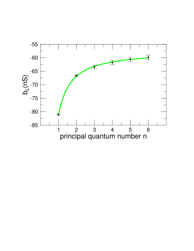
Figure 5: (color online). Dependence of the two-loop Bethe logarithm $b_{L}(nS)$ on the principal quantum number $n$. The explicit numerical results [Eq. (34)] are displayed together with a three-parameter fit of the form $-57.4-13.7/n-10.1/n^{2}$ from which one may infer $\lim_{n\to\infty}b_{L}(nS)=-57(2)$. Quantities plotted along the abscissa and the ordinate axis are (of course) dimensionless.

IV AMBIGUITY IN THE DEFINITION OF $B_{60}$

Low Low (1952) was the first to point out that the definition of an atomic energy level becomes problematic at the order of $\alpha^{8}$ [more specifically, $\alpha^{2}\,(Z\alpha)^{6}\,m$], and that it becomes necessary at this level of accuracy to consider the contribution of nonresonant energy levels to the elastic scattering cross section. In Jentschura and Mohr (2002), it has been stressed that nonresonant effects are enhanced in differential as opposed to total cross section, leading to corrections of order $\alpha^{2}\,(Z\alpha)^{4}\,m$. Related issues have recently attracted some attention (see also the discussion in Sec. I), and there is even a connection to the two-loop corrections of order $\alpha^{2}\,(Z\alpha)^{6}\,m$, as we discuss in the following. Namely, as pointed out in Jentschura et al. (2002a), the two-loop self-energy contains contributions which result from squared decay rates.

For excited reference states, the nonrelativistic two-loop self-energy (14) contains imaginary contributions which are generated by both the $\omega_{1}$- as well as the $\omega_{2}$-integrations. The imaginary part of the one-photon self-energy is generated by a pole contribution and leads to the decay rate which is the imaginary part of the self-energy. Consequently, real contributions to the two-photon self-energy which result as a product of two imaginary contributions are naturally referred to as squared decay rates. These are natural contributions to the two-loop self-energy shift in the order of $\alpha^{2}\,(Z\alpha)^{6}\,m$ and cannot be associated in a unique manner with one and only one atomic level. Roughly speaking, the problems in the interpretation originate from the fact that the Gell–Mann–Low–Sucher Gell-Mann and Low (1951); Sucher (1957) formalism involves a priori asymptotic states with an infinite lifetime (vanishing decay rate). Furthermore, it has been mentioned Jentschura et al. (2002b) that problematic issues persist even if the concept of an atomic energy is generalized to a resonance with a finite width—i.e., even if the canonical concept of a pole of the resolvent on the second Riemann sheet Cohen-Tannoudji et al. (1989, 1992) is used for the definition of an atomic resonance. In general, the squared decay rates illustrate that we are reaching the limit of the proper definition of atomic energy levels in considering higher-order two-loop binding corrections.

In Jentschura et al. (2002a), the squared decay rates have been analyzed in some detail. There are four specific terms out of the nine in curly brackets in Eq. (14) which give rise to squared decay rates. We list these terms here with a special emphasis on the higher excited $3S$ state, following the notation introduced in Jentschura et al. (2002a). In the following formulas, the physical dimensions of all energies and frequencies are restored [cf. Eq. (16)], and we have for the first term ${\mathcal{T}}_{1}({3S})$, which is the analog of Eq. (4) of Jentschura et al. (2002a):

$${\mathcal{T}}_{1}({3S})=\lim_{\delta\to 0^{+}}-\left(\frac{2\,\alpha}{3\,\pi\,m^{2}}\right)^{2}\,\int_{0}^{\epsilon_{1}}{\rm d}\omega_{1}\,\omega_{1}\,\int_{0}^{\epsilon_{2}}{\rm d}\omega_{2}\,\omega_{2}\,$$ (35a)

$$\times\left<{3S}\left|p^{i}\,\frac{1}{H-{\rm i}\,\delta-E_{3S}+\omega_{1}}\,p^{j}\,\frac{1}{H-E_{3S}+\omega_{1}+\omega_{2}}\,p^{i}\,\frac{1}{H-{\rm i}\,\delta-E_{3S}+\omega_{2}}\,p^{j}\right|{3S}\right>\,.$$

For the analog of Eq. (8) of Jentschura et al. (2002a), we have

$${\mathcal{T}}_{2}({3S})=\lim_{\delta\to 0^{+}}-\left(\frac{2\,\alpha}{3\,\pi\,m^{2}}\right)^{2}\,\int_{0}^{\epsilon_{1}}{\rm d}\omega_{1}\,\omega_{1}\,\int_{0}^{\epsilon_{2}}{\rm d}\omega_{2}\,\omega_{2}\,$$ (35b)

$$\times\left<{3S}\left|p^{i}\,\frac{1}{H-{\rm i}\,\delta-E_{3S}+\omega_{1}}\,p^{i}\,\left(\frac{1}{H-E_{3S}}\right)^{\prime}\,p^{j}\,\frac{1}{H-{\rm i}\,\delta-E_{3S}+\omega_{2}}\,p^{j}\right|{3S}\right>\,,$$

and we also have [see Eq. (15) of Jentschura et al. (2002a)]

$${\mathcal{T}}_{3}({3S})=\lim_{\delta\to 0^{+}}\left(\frac{2\,\alpha}{3\,\pi\,m^{2}}\right)^{2}\,\int_{0}^{\epsilon_{1}}{\rm d}\omega_{1}\,\omega_{1}\,\int_{0}^{\epsilon_{2}}{\rm d}\omega_{2}\,\omega_{2}\,$$ (35c)

$$\times\left<{3S}\left|p^{i}\,\frac{1}{H-{\rm i}\,\delta-E_{3S}+\omega_{1}}\,p^{i}\,\right|{3S}\right>\,\left<{3S}\left|p^{j}\,\left(\frac{1}{H-{\rm i}\,\delta-E_{3S}+\omega_{2}}\right)^{2}\,p^{j}\right|{3S}\right>\,.$$

The last relevant term is [see Eq. (17) of Jentschura et al. (2002a)]

$${\mathcal{T}}_{4}({3S})=\lim_{\delta\to 0^{+}}\left(\frac{2\,\alpha}{3\,\pi\,m^{2}}\right)^{2}\,\int_{0}^{\epsilon_{1}}{\rm d}\omega_{1}\,\omega_{1}\,\int_{0}^{\epsilon_{2}}{\rm d}\omega_{2}\,\omega_{2}\,$$ (35d)

$$\times\left<{3S}\left|p^{i}\,\frac{1}{H-{\rm i}\,\delta-E_{3S}+\omega_{1}}\,\frac{1}{H-{\rm i}\,\delta-E_{3S}+\omega_{2}}\,p^{i}\right|{3S}\right>\,.$$

Here, $H$ is the Schrödinger Hamiltonian. We now proceed to analyze the squared decay rates generated by the terms ${\cal T}_{i}$ ($i=1,\dots,4$) in some detail. It should be reemphasized here that the main contributions to the energy shift generated by the ${\cal T}_{i}$ have already been analyzed in Sec. III. However, the prescriptions (27) and (28) lead to a complete neglect of the (squared) imaginary contributions. Consequently, we here “pick up” only the terms of the “squared-decay” type—i.e., the terms generated by the infinitesimal half-circles around the poles at $\omega_{1}=E_{3S}-E_{2P}$ and $\omega_{2}=E_{3S}-E_{2P}$. For the evaluation of these squared pole terms, specification of the infinitesimal imaginary part $-{\rm i}\,\delta$ is required in order to fix the sign of the pole contribution. This procedure of extracting squared imaginary parts leads to the terms ${\cal C}_{i}$ ($i=1,\dots,4$), respectively rem (b).

We now proceed to analyze the squared decay rates generated by the terms ${\cal T}_{i}$ ($i=1,\dots,4$) in some detail. The term ${\cal T}_{1}$ is due to the diagram with crossed loops in Fig. 1(A). For the contribution $C_{1}({3S})$ generated by the poles at $\omega_{1}=E_{3S}-E_{2P}$ and $\omega_{2}=E_{3S}-E_{2P}$ in ${\mathcal{T}}_{1}({2P})$, we obtain

$$C_{1}({3S}) = \alpha^{2}\,\frac{4}{9m^{4}}\left(E_{3S}-E_{2P}\right)^{2}\,|\langle{2P}|\bm{p}|{3S}\rangle|^{2}$$ (36)

$$\times\left<{2P}\left|p^{i}\,\frac{1}{H+E_{3S}-2\,E_{2P}}\,p^{i}\right|{2P}\right>$$

$$= \frac{2^{5}}{3^{3}\,5^{8}}\,\alpha^{2}\,(Z\alpha)^{6}\,m\,{\cal M}_{1}\,,$$

where we define $|{2P}\rangle$ to be the state with magnetic quantum number (angular momentum projection) $m=0$. This explains the additional factor of $3$ in comparison to Eq. (5) of Jentschura et al. (2002a). The factor originates from the summation over magnetic quantum numbers of the $|{2P}\rangle$ state, and we reemphasize that we understand by $|{2P}\rangle$ only the state with magnetic quantum number (angular momentum projection) $m=0$. The matrix element ${\cal M}_{1}$ reads

$${\cal M}_{1}=\frac{1}{m}\,\left<{2P}\left|\,p^{i}\,\frac{1}{H+E_{3S}-2\,E_{2P}}\,p^{i}\,\right|{2P}\right>=0.697\,,$$ (37)

and we have for the well-known dipole matrix element

$$\left|\left<{2P}\left|\frac{\bm{p}}{m}\right|{3S}\right>\right|^{2}=\frac{2^{9}\,3^{3}}{5^{10}}\,(Z\alpha)^{2}\,.$$ (38)

Note that the contribution $C_{1}$ lacks the factors $\pi$ in the denominator which are characteristic of other two–loop corrections: these are compensated by additional factors of $\pi$ in the numerator that characterize the pole contributions.

The rainbow diagram in Fig. 1(B) with the second loop inside the first does not create squared imaginary contributions. From the irreducible part of the loop-after-loop diagram in Fig. 1(C) (we exclude the reference state in the intermediate electron propagator), the term ${\cal T}_{2}$ is obtained. Again, picking up only those terms which are generated by the infinitesimal half-circles around the poles at $\omega_{1}=E_{3S}-E_{2P}$ and $\omega_{2}=E_{3S}-E_{2P}$, we obtain the contribution $C_{2}({3S})$ involving squared decay rates:

$$C_{2}({3S}) = \alpha^{2}\,\frac{4}{9m^{4}}\left(E_{3S}-E_{2P}\right)^{2}\,|\langle{2P}|\bm{p}|{3S}\rangle|^{2}$$ (39)

$$\times\left<{2P}\left|p^{i}\,\left(\frac{1}{H-E_{3S}}\right)^{\prime}\,p^{i}\right|{2P}\right>$$

$$= \frac{2^{5}}{3^{3}\,5^{8}}\,\alpha^{2}\,(Z\alpha)^{6}\,m\,{\cal M}_{2}\,,$$

where the matrix element ${\cal M}_{2}$ reads

$${\cal M}_{2}=\frac{1}{m}\,\left<{2P}\left|\,p^{i}\,\left(\frac{1}{H-E_{3S}}\right)^{\prime}\,p^{i}\,\right|{2P}\right>=0.490\,.$$ (40)

The prime in the reduced Green function indicates that the $3S$ state is excluded from the sum over intermediate states, and it should not be confused with the notation used in Sec. III, where the prime was used to denote scaled dimensionless instead of dimensionful quantities.

From the derivative term (reducible part of the loop-after-loop diagram), we obtain

$$C_{3}({2P}) = -\alpha^{2}\,\frac{4}{3m^{4}}\left(E_{3S}-E_{2P}\right)\,|\langle{2P}|\bm{p}|{3S}\rangle|^{4}\,$$ (41)

$$= -\frac{2^{17}\,3^{3}}{5^{19}}\,\alpha^{2}\,(Z\alpha)^{6}\,m\,.$$

In order to derive the imaginary parts, one should remember that the squared propagator originates from a differentiation of a single propagator with respect to the energy. An integration by parts is helpful.

The last contribution of the “squared-decay” type—it originates from the “seagull term” characteristic of NRQED—is ${\cal T}_{4}$. The corresponding ${\cal C}$-term is

$$C_{4}({3S}) = -\alpha^{2}\,\frac{4}{3m^{3}}\left(E_{3S}-E_{2P}\right)^{2}\,|\langle{2P}|\bm{p}|{3S}\rangle|^{2}\,$$ (42)

$$= -\frac{2^{5}}{3^{2}\,5^{8}}\,\alpha^{2}\,(Z\alpha)^{6}\,m\,.$$

Adding all contributions, we obtain a shift of

$$\sum_{i=1}^{4}C_{i}({3S})=\left(\frac{\alpha}{\pi}\right)^{2}\,\frac{(Z\alpha)^{6}\,m}{3^{3}}\,(-0.00151)$$ (43)

for the $3S$ level. The numerical value is tiny; for $Z=1$ the shift amounts to only

$$\delta^{2}\nu(3S)=-0.00565\,{\rm Hz}\,.$$ (44)

For the corresponding ambiguous contributions to the $B_{60}$-coefficient [see Eqs. (2) and (43)], we use the notation

$$\delta^{2}B_{60}(3S)=-0.00151\,.$$ (45)

For the $4S$ state, we have to take into account the decays into the $2P$ and $3P$ states. For example, the contribution $C_{1}(4S)$ reads

$$C_{1}(4S) = \alpha^{2}\,\frac{4}{9m^{4}}\,\left\{\left(E_{\rm 4S}-E_{2P}\right)^{2}\,|\langle{2P}|\bm{p}|{\rm 4S}\rangle|^{2}\,\left<{2P}\left|p^{i}\,\frac{1}{H+E_{\rm 4S}-2\,E_{2P}}\,p^{i}\right|{2P}\right>\right.$$ (46)

$$\quad\left.+\left(E_{\rm 4S}-E_{\rm 3P}\right)^{2}\,|\langle{\rm 3P}|\bm{p}|{\rm 4S}\rangle|^{2}\,\left<{\rm 3P}\left|p^{i}\,\frac{1}{H+E_{\rm 4S}-2\,E_{\rm 3P}}\,p^{i}\right|{\rm 3P}\right>\right\}$$

$$+\alpha^{2}\,\frac{8}{9m^{4}}\,(E_{\rm 4S}-E_{2P})\,(E_{\rm 4S}-E_{\rm 3P})\,{\rm Re}\left(\langle{\rm 4S}|p^{j}|{2P}\rangle\,\left<{2P}\left|p^{i}\,\frac{1}{H+E_{\rm 4S}-E_{\rm 3P}-E_{2P}}\,p^{i}\right|{\rm 3P}\right>\,\langle{\rm 3P}|p^{j}|{\rm 4S}\rangle\right)$$

$$= \left(\frac{\alpha}{\pi}\right)^{2}\,\frac{(Z\alpha)^{6}\,m}{4^{3}}\,(0.00108)\,.$$

Table 1: Sample values of the $g$ function, defined in Eq. (25), for the $nS$ states with $n=1,\dots,6$. Multiplication by a factor of $n^{3}$ approximately accounts for the $n$-dependence, in agreement with the $n^{-3}$-type scaling of the two-loop correction as implied by Eq. (1).

$\omega$	$g_{1S}$	$8\,g_{2S}$	$27\,g_{{3S}}$	$64\,g_{4S}$	$125\,g_{{3S}}$	$216\,g_{6S}$
0	0.000 00	0.000 00	0.000 0	0.000 0	0.000 0	0.000 0
5	-10.281 60	-10.367 94	-10.450 1	-10.490 8	-10.522 6	-10.546 0
20	-16.560 34	-16.415 97	-16.393 4	-16.385 1	-16.386 1	-16.386 7
80	-22.714 02	-22.439 66	-22.372 0	-22.345 5	-22.332 0	-22.326 3
180	-26.232 35	-25.923 09	-25.848 0	-25.813 6	-25.798 1	-25.789 5

Table 2: Squared decay rates are extracted as the squared bound-state pole terms from the terms ${\cal T}_{1}$—${\cal T}_{4}$ in Eqs. (35a)—(35d). Explicit formulas ($3S$ state) for the terms ${\cal C}_{i}$ ($i=1,\dots,4$) are given in Eqs. (36)—(42). All contributions ${\cal C}_{i}$ scale as $Z^{6}$, whereas the decay rates $\Gamma$ given in the eighth column scale as $Z^{4}$. Numerical values are given for $Z=1$. The decay rates may be derived in the standard way [see the derivation of Fermi’s golden rule as given in Eqs. (2.103)—(2.118) of Sakurai (1967)]. We only indicate approximate values for $\Gamma$, without relativistic corrections. For the $2P_{1/2}$ states, a detailed calculation leads to $\Gamma(2P_{1/2})=0.9970942\,Z^{4}\,{\rm MHz}$ Sapirstein et al. (2004). For any given state, the squared decay rates $\delta^{2}\nu$ are about seven to eight orders of magnitude smaller than the width $\Gamma$. All states listed in the table may decay via the $E1$ mode, wherefore the decay rates as well as the ambiguities $\delta^{2}\nu$ are formally of the same order-of-magnitude [$\alpha\,(Z\alpha)^{4}\,m$ and $\alpha^{2}\,(Z\alpha)^{6}\,m$, respectively]. However, the numerical coefficients differ by two orders of magnitude; $S$ states typically have a much longer lifetime.

state	${\cal C}_{1}$	${\cal C}_{2}$	${\cal C}_{3}$	${\cal C}_{4}$	$\delta^{2}\nu=\sum_{i=1}^{4}{\cal C}_{i}$	$\delta^{2}B_{60}$	$\Gamma$	$\tau$
${2P}$	$1.42208$ Hz	$2.06790$ Hz	$-1.00843$ Hz	$-4.84593$ Hz	$-2.36438$ Hz	$-0.18789$	$99.76$ MHz	$0.16\times 10^{-8}$ s
$3P$	$0.50353$ Hz	$0.06037$ Hz	$-0.12787$ Hz	$-2.00952$ Hz	$-1.57349$ Hz	$-0.42202$	$30.21$ MHz	$0.53\times 10^{-8}$ s
${3S}$	$0.00210$ Hz	$0.00148$ Hz	$-0.00018$ Hz	$-0.00565$ Hz	$-0.00564$ Hz	$-0.00151$	$1.00$ MHz	$15.83\times 10^{-8}$ s
$4S$	$0.00170$ Hz	$-0.00100$ Hz	$-0.00015$ Hz	$-0.01019$ Hz	$-0.00964$ Hz	$-0.00613$	$0.70$ MHz	$22.65\times 10^{-8}$ s

The sum of $C_{1,\dots,4}$ for the $4S$ state of hydrogenlike systems with (low) nuclear charge $Z$ is

$$\sum_{i=1}^{4}C_{i}(4S)=\left(\frac{\alpha}{\pi}\right)^{2}\,\frac{(Z\alpha)^{6}\,m}{4^{3}}\,(-0.00613)\,.$$ (47)

For atomic hydrogen ($Z=1$), this correction evaluates to

$$\delta^{2}\nu(4S)=-0.00964\,{\rm Hz}\,.$$ (48)

This is numerically larger than the corresponding effect for ${3S}$ [see Eq. (44)]. We have

$$\delta^{2}B_{60}(4S)=-0.00613\,.$$ (49)

Although self-energy corrections canonically scale as $n^{-3}$ [see Eq. (1)], the coefficient in this case grows so rapidly with $n$ that the correction is enhanced for $4S$ in comparison to $3S$. Further detailed information can be found in Table 2. We also take the opportunity to clarify that numerical values for squared decay as given in Jentschura et al. (2002a) (for $2P$ and $3P$ states) should be understood as given in inverse seconds rather than Hz (see also the discussion near the beginning of Sec. III).

V FURTHER CONTRIBUTIONS TO $B_{60}$

The coefficient $B_{60}$ can be represented as the sum

$$B_{60}=b_{L}+b_{M}+b_{F}+b_{H}+b_{\rm VP}\,.$$ (50)

The two-loop Bethe logarithm $b_{L}$ comes from the region where both photon momenta are small and has been the subject of this work. $b_{M}$ stems from an integration region where one momentum is large $\sim m$, and the second momentum is small. This contribution is given by a Dirac $\delta$ correction to the Bethe logarithm [see also Eq. (21) and Ref. Jentschura (2003b)]. It has already been derived in Pachucki (2001) but not included in the theoretical predictions for the Lamb shift:

$$b_{M}=\frac{10}{9}\,N(nS)\,.$$ (51)

As has already been mentioned in Pachucki and Jentschura (2003), the contributions $b_{F}$ and $b_{H}$ originate from a region where both photon momenta are large $\sim m$, and the electron momentum is small and large respectively. Finally, $b_{\rm VP}$ is a contribution from diagrams that involve a closed fermion loop. None of these effects have been calculated as yet. On the basis of our experience with the one- and two-loop calculations we estimate the magnitude of these uncalculated terms to be of the order of 15%. For higher excited states ($3S,\dots,6S$), the $15\,\%$ uncertainty due to unknown contributions is larger than the ambiguity $\delta^{2}B_{60}$ listed in Table 2.

Concerning logarithmic two-loop vacuum-polarization effects Pachucki (2001), we mention that the contribution of the two-loop self-energy diagrams to $B_{61}$ for the $1S$ state reads $49.8$, whereas the diagrams that involve a closed fermion loop amount to $0.6$. Concerning the one-loop higher-order binding correction $A_{60}(1S)$ (analog of $B_{60}$) it is helpful to consider that the result for $1S$ is $-30.92415(1)$ (see Refs. Pachucki (2001); Jentschura et al. (1999)); this is the sum of a contribution due to low-energy virtual photons of $-27.3$ (Pachucki, 2001, Eq. (5.116)), and a relatively small high-energy term of about $-3.7$ (Pachucki, 2001, Eq. (6.102)). In estimating these contributions, we follow Pachucki and Jentschura (2003).

This leads to the following overall result for the $B_{60}$ coefficients, where the first two results ($1S$ and $2S$) are quoted from Pachucki and Jentschura (2003), and the latter results are obtained within the current investigation:

$$B_{60}(1S) = -61.6(3)\pm 15\%\,,$$ (52a)

$$B_{60}(2S) = -53.2(3)\pm 15\%\,,$$ (52b)

$$B_{60}(3S) = -51.9(6)\pm 15\%\,,$$ (52c)

$$B_{60}(4S) = -51.0(8)\pm 15\%\,,$$ (52d)

$$B_{60}(5S) = -50.3(8)\pm 15\%\,,$$ (52e)

$$B_{60}(6S) = -49.8(8)\pm 15\%\,.$$ (52f)

The values are in numerical agreement with those used in latest adjustment of the fundamental physical constants MoT ; these are based on an extrapolation of the results obtained for $n=1,2$ Pachucki and Jentschura (2003) to higher $n$, using a functional form $a+b/n$, with an extra uncertainty added in order to account for the somewhat incomplete form of the functional form used in the extrapolation. We here confirm the validity of the approach taken in MoT by our explicit numerical calculation.

VI CONCLUSIONS

The calculation of binding two-loop self-energy corrections has received considerable attention within the last decade Pachucki (1993b, 1994); Eides et al. (1994); Eides and Shelyuto (1995). As outlined in Sec. I, there is an intuitive physical reason why a reliable understanding of the two-loop energy shift requires the calculation of all logarithmic as well as nonlogarithmic corrections through the order of $\alpha^{2}\,(Z\alpha)^{6}\,m$. It is the order of $\alpha^{2}\,(Z\alpha)^{6}\,m$ which is the “natural” order-of-magnitude for the two-loop self-energy effect from the point of view of nonrelativistic quantum electrodynamics (NRQED); i.e., low-energy virtual photons begin to contribute at this order only, whereas effects of lower order [$\alpha^{2}\,(Z\alpha)^{4}\,m$ and $\alpha^{2}\,(Z\alpha)^{5}\,m$] are mediated exclusively by high-energy virtual quanta.

In Sec. II, we recall known lower-order coefficients for $S$ states, as well as logarithmic corrections. The formulation of the problem within NRQED Caswell and Lepage (1986) and the actual numerical evaluation of the two-loop Bethe logarithms $b_{L}$ for higher excited $S$ states is discussed in Sec. III. Numerical results for $b_{L}$ are given in Eq. (34). As shown in Fig. 5, the dependence of these results on the principal quantum number follows a pattern recently observed quite universally for binding corrections to radiative bound-state energy shifts Jentschura (2003b); Jentschura et al. (2003). This permits an extrapolation of the results to higher principal quantum numbers, which is useful for the determination of fundamental constants MoT .

There is a certain ambiguity in the definition of the two-loop nonlogarithmic coefficient $B_{60}$ due to squared decay rates (Sec. IV); this aspect has previously been considered in Jentschura et al. (2002a) for $P$ states. Here, the treatment of the squared decay rates is generalized to excited $S$ states. The ambiguity, while formally of the order of $\alpha^{2}\,(Z\alpha)^{6}\,m$, is shown to be barely significant for $S$ states (see Table 2), due to small prefactors.

Numerical estimates of the total $B_{60}$-coefficient for excited $nS$ states ($n=1,\dots,6$) are given in Eq. (52). These results improve our theoretical knowledge of the hydrogen spectrum. On the occasion, we would also like to mention ongoing efforts regarding the calculation of binding three-loop corrections of order $\alpha^{3}\,(Z\alpha)^{5}$ Eides and Shelyuto (2004). At $Z=1$, these binding three-loop corrections are of the same order-of-magnitude ($\alpha^{8}$) as the two-loop Bethe logarithms discussed here. There is considerable hope that in the near future, our possibilities for a self-consistent interpretation of high-precision laser spectroscopic experiments may be enhanced significantly via a combination of ongoing experiments at Paul Scherrer Institute (PSI), Laboratoire Kastler–Brossel and Max–Planck–Institute for Quantum Optics, whose purpose is a much improved Lamb-shift measurement ($1S$–$2S$– and $1S$–${3S}$–transitions combined with an improved knowledge of the proton charge radius as derived from the PSI muonic hydrogen experiment). The comparison of numerous transitions in hydrogenlike systems with theory may also help in this direction as it allows for an evaluation of the proton charge radius using an overdetermined system of equations, provided that theoretical Lamb-shift values are used as input data for the systems of equations rather than variables for which the systems should be solved [see, e.g., Eqs. (2) and (3) of Udem et al. (1997)].

Finally, we would like comment on the relation of the analytic approach ($Z\alpha$ expansion) pursued here and numerical calculations of the self-energy at low nuclear charge $Z$, which avoid the $Z\alpha$ expansion and which have been carried out on the one-loop level for high nuclear charge numbers $Z$ Mohr (1974), with recent extensions to the numerically more problematic regime of low $Z$ Jentschura et al. (1999). One might note that traditionally, the most accurate Lamb-shift values at low $Z$ have been obtained via a combination of analytic and numerical techniques—i.e., by using both numerical data obtained for high $Z$ and known analytic coefficients from the $Z\alpha$ expansion Mohr (1975). (This is one of the main motivations for pursuing both numerical and analytic calculations of the two-loop self energy, in addition to the obvious requirement for an additional cross-check of the two distinct approaches.) The general paradigm is the extrapolation of the self-energy remainder function obtained from high-$Z$ numerical data after the subtraction of known analytic terms; in many cases this extrapolation leads to more accurate predictions for the remainder at low $Z$ than the simple truncation of the $Z\alpha$ expansion alone. Various algorithms have been developed for this purpose (see, e.g., Mohr (1975); Ivanov and Karshenboim (2001)). Indeed, the combination of analytic and numerical techniques has recently proven to be useful in the context of binding corrections to the one-loop bound-electron $g$ factor Pachucki et al. (b), although direct numerical evaluations at $Z=1$ had been available before Yerokhin et al. (2002). Still, it was possible to improve the theoretical predictions for the $g$ factor self-energy remainder function at low $Z$ by an order of magnitude via a combination of the analytic and numerical approaches, in addition to the fact that an important cross-check of the analytic and the numerical approaches versus each other became feasible.