Abstract

In this talk I report on the results of a recent calculation of the $\alpha_{s}$ corrections to a three-point correlation function at the three-loop level in QCD perturbation theory, which allows one to extract the matrix element of $B^{0}-\bar{B}^{0}$ mixing with next-to-leading order accuracy [1]. The evaluation of mixing parameter at NLO allows for a consistent analysis of $B^{0}-\bar{B}^{0}$ mixing since the coefficient functions of the effective Hamiltonian for this process are known with the necessary accuracy.

Presently the pattern of CP violation in the Standard Model is under thorough experimental study in dedicated experiments by BABAR collaboration at SLAC (e.g. [2, 3]) and BELLE collaboration at KEK (e.g. [4, 5]). The standard mechanism of CP violation to be primarily tested is a Cabibbo-Kobayashi-Maskawa paradigm with mixing of (at least) three quark generations (for review, see e.g. [6]). At the hadronic level the fact of quark mixing mainly reveals itself as mixing of neutral pseudoscalar mesons. The most famous system where mixing occurs and has been studied in much detail is the system of neutral kaons. Study of $K^{0}-\bar{K}^{0}$ mixing strongly constrained the physics of heavy particles and allowed to estimate the numerical value of the charm quark mass from the requirement of GIM cancellation before the experimental discovery of charm (see e.g. [7]). At present the experimental studies of CP violation shifted to the realm of heavy mesons for which they are considered more promising. In particular, recent experimental results for heavy charmed mesons $D(\bar{u}c)$ are encouraging [8]. However the systems of $B_{d}(\bar{d}b)$ and $B_{s}(\bar{s}b)$ mesons are the most promising laboratory for performing a precision analysis of CP violation and mixing both experimentally and theoretically [9].

Mixing in any system of neutral pseudoscalar mesons is described by a 2x2 effective Hamiltonian or mass operator $\left(M-i\Gamma/2\right)_{ij}$, $\{i,j\}=\{1,2\}$ where $M$ is related to the mass spectrum of the system and $\Gamma$ describes the widths of the mesons. In the presence of flavor violating interactions ($\Delta B=2$ in our particular case) the effective Hamiltonian acquires non-diagonal terms. The difference between the values of the mass eigenstates of $B$ mesons $\Delta m=M_{heavy}-M_{light}\approx 2\left|M_{12}\right|$ is precisely measured $\Delta m=0.489\pm 0.005(stat)\pm 0.007(syst)~{}ps^{-1}$ [10]. With an accurate theoretical description of the mixing, it can be used to extract the top quark CKM parameters. In Wolfenstein’s parametrization the CKM matrix elements reveal a hierarchy in magnitude. In terms of Cabibbo angle $\lambda\approx 0.22$, this parametrization of the CKM matrix $V$ reads

$$V\simeq\left(\matrix{1-{1\over 2}\lambda^{2}&\lambda&A\lambda^{3}\left(\rho-i\eta\right)\cr-\lambda(1+iA^{2}\lambda^{4}\eta)&1-{1\over 2}\lambda^{2}&A\lambda^{2}\cr A\lambda^{3}\left(1-\rho-i\eta\right)&-A\lambda^{2}&1\cr}\right)$$

Here

$$V_{us}=\lambda,\quad V_{cb}=A\lambda^{2},\quad V_{ub}=A\lambda^{3}(\rho-i\eta),\quad V_{td}=A\lambda^{3}(1-\bar{\rho}-i\bar{\eta}).$$

While $|V_{cb}|$ and $|V_{ub}|$ can be extracted from semileptonic $B$ decays, $|V_{td}|$ is at present probed in the process of $B_{d}^{0}$–${\bar{B}_{d}^{0}}$ mixing.

The expression for the effective Hamiltonian describing $\Delta B=2$ transitions is known at next-to-leading order (NLO) in QCD perturbation theory of the Standard Model [11]

$$H_{\mbox{eff}}^{\triangle B=2} = \frac{G_{F}^{2}M_{W}^{2}}{4\pi^{2}}\left({V_{tb}}^{*}V_{td}\right)^{2}\eta_{B}S_{0}(x_{t})\times\left[\alpha_{s}^{(5)}(\mu)\right]^{-6/23}\left[1+\frac{\alpha_{s}^{(5)}(\mu)}{4\pi}J_{5}\right]{\cal O}(\mu)$$

where $G_{F}$ is a Fermi constant, $M_{W}$ is the W-boson mass, $\eta_{B}=0.55\pm 0.1$ [12], $J_{5}=1.627$ in the naive dimensional regularization (NDR) scheme, $S_{0}(x_{t})$ is the Inami-Lim function [13], and ${\cal O}(\mu)=(\bar{b}_{L}\gamma_{\sigma}d_{L})(\bar{b}_{L}\gamma_{\sigma}d_{L})(\mu)$ is a local four-quark operator at the normalization point $\mu$. Mass splitting of heavy and light mass eigenstates is

$$\Delta m=2|\langle\bar{B}^{0}|H_{\mbox{eff}}^{\triangle B=2}|B^{0}\rangle|=~{}\!\!{\cal C}\left[\alpha_{s}^{(5)}(\mu)\right]^{-6/23}\left[1+\frac{\alpha_{s}^{(5)}(\mu)}{4\pi}J_{5}\right]\langle\bar{B}^{0}|{\cal O}(\mu)|B^{0}\rangle$$

where we introduced a constant ${\cal C}=G_{F}^{2}M_{W}^{2}\left({V_{tb}}^{*}V_{td}\right)^{2}\eta_{B}m_{B}S_{0}(x_{t})/\left(4\pi^{2}\right)$. The largest uncertainty in calculation of the mass splitting is introduced by the hadronic matrix element ${\cal A}=\langle\bar{B}^{0}|{\cal O}(\mu)|B^{0}\rangle$ that is poorly known [10]. The evaluation of this matrix element is a genuine non-perturbative task, which should be approached with some non-direct techniques. The simplest approach (“factorization”) [14] reduces the matrix element ${\cal A}$ to the product of simpler matrix elements measured in leptonic $B$ decays

$${\cal A}^{f}=\frac{8}{3}\langle\bar{B}^{0}|\bar{b}_{L}\gamma_{\sigma}d_{L}|0\rangle\langle 0|\bar{b}_{L}\gamma^{\sigma}d_{L}|B^{0}\rangle=\frac{2}{3}f_{B}^{2}m_{B}^{2}$$ (1)

where the decay constant $f_{B}$ is defined by $\langle 0|\bar{b}_{L}\gamma_{\mu}d_{L}|B^{0}({\bf p})\rangle=ip_{\mu}f_{B}/2$ and $m_{B}$ is the $B^{0}$ meson mass. A deviation from the factorization ansatz is usually described by the parameter $B_{B}$ defined as ${\cal A}=B_{B}{\cal A}^{f}$; in factorization $B_{B}=1$. The evaluation of this parameter (and the analogous parameter $B_{K}$ of $K^{0}-\bar{K}^{0}$ mixing) has long history. Many different results were obtained within approaches based on quark models, unitarity, ChPT. The approach of direct numerical evaluation on the lattice has also been used. The corresponding results can be found in the literature [15, 16, 17, 18, 19, 20, 21, 22].

In my talk I report on the results of the calculation of the hadronic mixing matrix elements using Operator Product Expansion (OPE) and QCD sum rule techniques for three-point functions [1, 16, 17, 18, 23, 24]. This approach is very close in spirit to lattice computations [21], which is a model-independent, first-principles method. The difference is that the QCD sum rule approach uses an asymptotic expansions of a Green’s function computed analytically while on the lattice the function itself can be numerically computed provided the accuracy of the technique is sufficient. The sum rule techniques also provide a consistent way of taking into account perturbative corrections to matrix elements which is needed to restore the RG invariance of physical observables usually violated in the factorization approximation [25].

To start with let me introduce the three-point correlation function

$$\Pi(p_{1},p_{2})=\int dxdy\langle 0|TJ_{\bar{B}}(x){\cal O}(0)\bar{J}_{B}(y)|0\rangle e^{ip_{2}x-ip_{1}y}$$ (2)

of the relevant $\Delta B=2$ operator ${\cal O}(\mu)$ and interpolating currents for the $B^{0}$-meson $J_{B}=(m_{b}+m_{d})\bar{d}i\gamma_{5}b$. Here $m_{b}$ is the $b$ quark mass. The current $J_{B}$ is RG invariant and $J_{B}=\partial_{\mu}(\bar{d}\gamma_{\mu}\gamma_{5}b)$. The main relevant property of this current is $\langle 0|J_{B}(0)|B^{0}(p)\rangle=f_{B}m_{B}^{2}$ where $m_{B}$ is the $B$-meson mass. A dispersive representation of the correlator reads

$$\Pi(p_{1},p_{2})\equiv\Pi(p_{1}^{2},p_{2}^{2},q^{2})=\int\frac{\rho(s_{1},s_{2},q^{2})ds_{1}ds_{2}}{(s_{1}-p_{1}^{2})(s_{2}-p_{2}^{2})}$$ (3)

where $q=p_{2}-p_{1}$. For the analysis of $B^{0}-\bar{B}^{0}$ mixing within the sum rule framework this correlator can be computed at $q^{2}=0$.

Phenomenologically the matrix element $\langle\bar{B}^{0}|{\cal O}(\mu)|B^{0}\rangle$ determines the contribution of the $B$-mesons in the form of a double pole to the three-point correlator

$$\Pi(p_{1}^{2},p_{2}^{2},q^{2})=\frac{\langle J_{\bar{B}}|\bar{B}^{0}\rangle}{m_{B}^{2}-p_{1}^{2}}\langle\bar{B}^{0}|{\cal O}(\mu)|B^{0}\rangle\frac{\langle B^{0}|\bar{J}_{B}\rangle}{m_{B}^{2}-p_{2}^{2}}+\ldots$$ (4)

Because of technical difficulties of calculation, a practical way of extracting the $B^{0}-\bar{B}^{0}$ matrix element is to analyze the moments of the correlation function at ${p_{1}^{2}=p_{2}^{2}=0}$ at the point $q^{2}=0$

$$M(i,j)\equiv\frac{\partial^{i+j}\Pi(p_{1}^{2},p_{2}^{2},0)}{i!j!\partial p_{1}^{2i}\partial p_{2}^{2j}}=\int\frac{\rho(s_{1},s_{2},0)ds_{1}ds_{2}}{s_{1}^{i+1}s_{2}^{j+1}}\,.$$

A theoretical computation of these moments reduces to an evaluation of single scale vacuum diagrams and can be done analytically with available tools for the automatic computation of multi-loop diagrams. Note that masses of light quarks are small (e.g. [26]) and can be accounted for as small perturbation which is relevant for the problem of $B_{s}$ meson mixing [27].

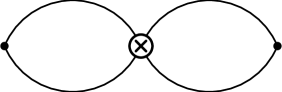
Figure 1: Perturbation theory diagram at LO

The leading contribution to the asymptotic expansion is given by the diagram shown in Fig. 1. At the leading order in QCD perturbation theory the three-point function $\Pi(p_{1},p_{2})$ of Eq. (2) completely factorizes

$$\Pi(p_{1},p_{2})=\frac{8}{3}\Pi_{\mu}(p_{1})\Pi^{\mu}(p_{2})$$ (5)

into a product of the two-point correlators $\Pi_{\mu}(p)$

$$\Pi_{\mu}(p)=p_{\mu}\Pi(p^{2})=\int dxe^{ipx}\langle 0|TJ_{\bar{B}}(x)\bar{b}_{L}\gamma_{\mu}d_{L}(0)|0\rangle.$$ (6)

At LO the calculation of moments is straightforward since the double spectral density $\rho(s_{1},s_{2},q^{2})$ is explicitly known in this approximation. Indeed, using dispersion relation for the two-point correlator

$$\Pi(p^{2})=\int_{m^{2}}^{\infty}\frac{\rho(s)ds}{s-p^{2}},\quad\rho(s)=\frac{3}{16\pi^{2}}m^{2}\left(1-\frac{m^{2}}{s}\right)^{2}$$ (7)

one obtains the LO double spectral density in a factorized form

$$\rho^{\rm LO}(s_{1},s_{2},q^{2})=\frac{8}{3}(p_{1}\cdot p_{2})\rho(s_{1})\rho(s_{2})=\frac{4}{3}(s_{1}+s_{2}-q^{2})\rho(s_{1})\rho(s_{2})\ .$$ (8)

Thus, all PT contributions are of the factorizable form at LO. First non-factorizable contributions to Eq. (3) appear at NLO. Of course, at NLO there are also the factorizable diagrams. Note that the classification of diagrams in terms of their factorizability is consistent as both classes are independently gauge and RG invariant.

Consider first the NLO factorizable contributions that are given by the product of two-point correlation functions from Eq. (6), as shown in Fig. 2. Analytical expression for such contributions can be obtained as follows. Writing $\Pi(p^{2})=\Pi_{\rm LO}(p^{2})+\Pi_{\rm NLO}(p^{2})$ one finds

$$\Pi_{\rm NLO}^{f}(p_{1},p_{2})=\frac{8}{3}(p_{1}.p_{2})(\Pi_{\rm LO}(p_{1}^{2})\Pi_{\rm NLO}(p_{2}^{2})+\Pi_{\rm NLO}(p_{1}^{2})\Pi_{\rm LO}(p_{2}^{2})).$$ (9)

Since the spectral density of the correlator $\Pi_{\rm NLO}(p^{2})$ is known analytically the problem of the NLO analysis in factorization is completely solved. Even a NNLO analysis of factorizable diagrams is possible as several moments of two-point correlators are known analytically. Others can be obtained numerically from the approximate spectral density [28].

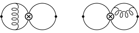
Figure 2: Factorizable diagrams at NLO

The NLO analysis of non-factorizable contributions within perturbation theory is the main point of my talk. The analysis amounts to the calculation of a set of three-loop diagrams (a typical diagram is presented in Fig. 3). These diagrams have been computed using the package MATAD for automatic calculation of Feynman diagrams [29]. The package is applicable only for computation of scalar integrals. the decomposition of the three-point amplitude into scalars is known [30]. A scalar function $A(p_{1},p_{2})$ of two four-momenta $p_{1}$ and $p_{2}$ can be expanded in a series over the scalar variable $p_{1}^{2}$, $p_{2}^{2}$ and $p_{1}\cdot p_{2}$ of the general form

$$A(p_{1},p_{2})=\sum_{j_{1},j_{2},j_{3}}a_{j_{1},j_{2},j_{3}}({p_{1}^{2}})^{j_{1}}({p_{2}^{2}})^{j_{2}}(p_{1}\cdot p_{2})^{j_{3}}.$$

For the coefficients $a_{j_{1},j_{2},j_{3}}$ one finds

$$a_{j_{1},j_{2},j_{3}}= \frac{1}{2^{j_{1}}2^{j_{2}}j_{3}!}\sum_{k=0}^{[j_{1}+\frac{j_{3}}{2}]}\frac{(-1)^{k-j_{1}}}{2^{2k+j_{2}-j_{1}}(2j_{1}+j_{3}-2k)!}$$

$$\sum_{l=max(0,k-j_{1})}^{min(k,k+j_{2}-j_{1})}\frac{(2j_{1}+j_{3}-2k+2l)!}{l!(j_{1}-k+l)!}\times$$

$$\frac{(1-\varepsilon)_{2j_{1}+j_{3}-2k+2l+1}(1-\varepsilon)_{j_{1}+j_{3}-k+l}}{(1-\varepsilon)_{2j_{1}+j_{3}-2k+2l}(1-2\varepsilon)_{2j_{1}+j_{3}-2k+2l+1}}$$

$$\frac{(1-\varepsilon)_{2j_{1}+j_{3}-2k+l}(1-\varepsilon)_{1}(1-2\varepsilon)_{1}}{(1-\varepsilon)_{2j_{1}+j_{3}-k+l+1}(1-\varepsilon)_{j_{1}+j_{2}+j_{3}-k+l+1}}$$

$$\quad\times\triangle_{11}^{k}\triangle_{22}^{k+j_{2}-j_{1}}\triangle_{12}^{2j_{1}+j_{3}-2k}A(p_{1},p_{2})|_{p_{1}=p_{2}=0}$$

with

$$\triangle_{ij}=g^{\mu\nu}\frac{\partial^{2}}{\partial p_{i}^{\mu}p_{j}^{\nu}}.$$

Here $(a)_{b}$ stands for the Pochhammer symbol $(a)_{b}=\Gamma(a+b)/\Gamma(a)$ and $d=4-2\varepsilon$ is the spacetime dimension. The actual calculation has been performed with the computer algebra system FORM [31].

Renormalization of the local four-quark operator ${\cal O}$ entering the effective Hamiltonian has been done in dimensional regularization with an anticommuting $\gamma_{5}$.

Figure 3: A typical non-factorizable diagram at NLO

The renormalization of the operator ${\cal O}$ reads

$${\cal O}^{R}={\cal O}^{B}-\frac{\alpha_{s}}{4\pi}\frac{1}{\varepsilon}{\cal O}_{c}$$ (10)

with ${\cal O}_{c}=(\bar{b}_{L}\Gamma_{\mu\nu\alpha}t^{a}d_{L})(\bar{b}_{L}\Gamma^{\mu\nu\alpha}t^{a}d_{L})$. The color space matrices $t^{a}$ are the $SU_{c}(3)$ generators and $\Gamma_{\mu\nu\alpha}=(\gamma_{\mu}\gamma_{\nu}\gamma_{\alpha}-\gamma_{\alpha}\gamma_{\nu}\gamma_{\mu})/2$. Note that in four dimensional space-time the matrix $\Gamma_{\mu\nu\alpha}$ reduces to the expression $-i\epsilon_{\mu\nu\alpha\beta}\gamma^{\beta}\gamma_{5}$. This relation is however ill defined in $D$-dimensional spacetime of dimensional regularization. The renormalization of the factorizable contributions reduces to that of the $b$-quark mass $m$. We use the quark pole mass as a mass parameter of the calculation.

The expression for the “theoretical” moments reads

$$M_{th}(i,j)=\frac{m^{6}a_{ij}}{m^{2(i+j)}}\left(1+\frac{\alpha_{s}}{4\pi}\left(b^{f}_{ij}+b^{nf}_{ij}\right)\right)$$ (11)

where the quantities $a_{ij}$, $b^{f}_{ij}$ and $b^{nf}_{ij}$ represent LO, NLO factorizable and NLO nonfactorizable contributions as shown in Figs. 1-3. The NLO nonfactorizable contributions $b^{nf}_{ij}$ with $i+j\leq 7$ are analytically calculated in ref. [1] for the first time. The calculation required about 24 hours of computing time on a dual-CPU 2 GHz Intel Xeon machine. The calculation of higher moments is feasible but requires considerable optimization of the code. This work is in progress. The analytical result for the lowest finite moment $M_{th}(2,2)$ reads

$$a_{22}=\frac{1}{(16\pi^{2})^{2}}\left(\frac{8}{3}\right),\quad b^{f}_{22}=\frac{40}{3}+\frac{16\pi^{2}}{9}\,,$$ (12)

$$b^{nf}_{22}=S_{2}\frac{8366187}{17500}-\zeta_{3}\frac{84608}{875}-\pi^{2}\frac{33197}{52500}-\frac{426319}{315000}.$$

Here $S_{2}=\frac{4}{9\sqrt{3}}{\rm Cl}_{2}\left(\frac{\pi}{3}\right)=0.2604\ldots$, $\zeta_{3}=\zeta(3)$, and $\mu^{2}=m^{2}$. Higher moments contain the same transcendental entries $S_{2}$, $\zeta_{3}$, $\pi^{2}$ with different numerical coefficients. The numerical values for the moments are $b^{nf}_{ij}$: $b^{nf}_{2(2345)}=\{0.68,1.22,1.44,1.56\}$ and $b^{nf}_{3(34)}=\{1.96,2.25\}$. The above theoretical results are used to extract the non-perturbative parameter $B_{B}$ from the sum rules analysis.

The “phenomenological” side of the sum rules is given by the moments which can be inferred from Eq. (4)

$$M_{ph}(i,j)=\frac{8}{3}B_{B}\frac{f_{B}^{4}m_{B}^{2}}{m_{B}^{2(i+j)}}+{\cal O}\left(\frac{1}{(m_{B}^{2}+\Delta)^{i+1}m_{B}^{2j}},\frac{1}{(m_{B}^{2}+\Delta)^{j+1}m_{B}^{2i}}\right)$$

where the contribution of the $B$-meson is displayed explicitly. The remaining parts are the contributions due to higher resonances and the continuum which are suppressed due to the mass gap $\Delta$ in the spectrum model. A rough picture of the phenomenological spectrum is given in Fig. (4).

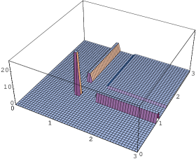
Figure 4: A model of phenomenological spectrum

For comparison we consider the factorizable approximation for both “theoretical”

$$M_{th}^{f}(i,j)=\frac{m^{6}a_{ij}}{m^{2(i+j)}}\left(1+\frac{\alpha_{s}}{4\pi}b^{f}_{ij}\right)$$ (13)

and “phenomenological” moments, which, by construction, are built from the moments of the two-point function of Eq. (6)

$$M_{ph}^{f}(i,j)=\frac{8}{3}\frac{f_{B}^{4}m_{B}^{2}}{m_{B}^{2(i+j)}}+...$$ (14)

According to standard QCD sum rule technique, the “theoretical” calculation is dual to the “phenomenological” one. Thus, Eq. (S0.Ex14) should be equivalent (in the sum rule sense) to Eq. (11). Also, in factorization, Eq. (14) is equivalent to Eq. (13). Now Eq. (13) and Eq. (11) differ only due to non-factorizable corrections. Therefore, the difference between Eq. (14) and Eq. (S0.Ex14) is because the residues differ from their factorized values.

To find the nonfactorizable addition to $B_{B}$ from the sum rules we form ratios of the total and factorizable contributions. On the “theoretical” side one finds

$$\frac{M_{th}(i,j)}{M_{th}^{f}(i,j)}=1+\frac{\alpha_{s}}{4\pi}\frac{b^{nf}_{ij}}{1+\frac{\alpha_{s}}{4\pi}b^{f}_{ij}}\,.$$ (15)

This ratio is mass-independent. On the “phenomenological” side we have

$$\frac{M_{ph}(i,j)}{M_{ph}^{f}(i,j)}=\frac{B_{B}+R_{B}(z^{j}+z^{i})+C_{B}z^{i+j}}{1+R^{f}(z^{j}+z^{i})+C^{f}z^{i+j}}$$ (16)

where $z=m_{B}^{2}/(m_{B}^{2}+\Delta)$ is a parameter that describes the suppression of higher state contributions. $\Delta$ is a gap between the squared masses of the $B$-meson and higher states. $R_{B}$, $C_{B}$, $R^{f}$ and $C^{f}$ are parameters of the model for higher state contributions within the sum rule approach. In order to extract the non-factorizable contribution to $B_{B}$ we write $B_{B}=1+\Delta B$. Similarly, one can parameterize contributions to “phenomenological” moments due to higher $B$-meson states by writing $R_{B}=R^{f}+\Delta R$ and $C_{B}=C^{f}+\Delta C$. Clearly, $\Delta B=\Delta R=\Delta C=0$ in factorization. We obtain

$$\frac{M_{ph}(i,j)}{M_{ph}^{f}(i,j)}=1+\frac{\Delta B+\Delta R(z^{j}+z^{i})+\Delta Cz^{i+j}}{1+R^{f}(z^{j}+z^{i})+C^{f}z^{i+j}}\,.$$ (17)

Comparing Eqs. (15) and (17) one sees how the perturbative non-factorizable correction $b^{nf}_{ij}$ is “distributed” among the phenomenological parameters of the spectrum. We extract $\Delta B$ by a combined fit of several “theoretical” and “phenomenological” moments. The final formula for the determination of $\Delta B$ reads

$$\frac{\alpha_{s}}{4\pi}b^{nf}_{ij}=\Delta B+\Delta R(z^{j-2}+z^{i-2})+\Delta Cz^{i+j-4}$$ (18)

where $\Delta R$ and $\Delta C$ are free parameters of the fit. We take $\Delta=0.4m_{B}^{2}$ for the $B$ meson two-point correlator. This corresponds to the duality interval of $1~{}{\rm GeV}$ in energy scale for the analysis based on finite energy sum rules [32]. The actual value of $\Delta B$ has been extracted using the least-square fit of all available moments. Estimating all uncertainties we finally find the NLO non-factorizable QCD corrections to $\Delta B$ due to perturbative contributions to the sum rules to be

$$\Delta B=(6\pm 1)\frac{\alpha_{s}(m)}{4\pi}$$

We checked the stability of the sum rules which lead to a prediction of $\Delta B$. For $m_{b}=4.8~{}{\rm GeV}$ and $\alpha_{s}(m_{b})=0.2$ [33] one finds $\Delta B=0.1$. The calculation can be further improved with the evaluation of higher moments. The result is sensitive to the parameter $z$ or to the magnitude of the mass gap $\Delta$ used in the parametrization of the spectrum.

In conclusion, the $B^{0}-\bar{B}^{0}$ mixing matrix element has been evaluated in the framework of QCD sum rules for three-point functions at NLO in perturbative QCD. The effect of radiative corrections on $B_{B}$ is under complete control within pQCD and amounts to approximately $+10$% of the factorized value.

References

• [1] J. G. Körner, A. I. Onishchenko, A. A. Petrov and A. A. Pivovarov, Phys. Rev. Lett. 91, 192002 (2003) [arXiv:hep-ph/0306032].
• [2] B. Aubert et al. [BABAR Collaboration], Phys. Rev. D 66, 032003 (2002) [arXiv:hep-ex/0201020].
• [3] B. Aubert et al. [BABAR Collaboration], Phys. Rev. Lett.  89, 201802 (2002)
• [4] K. Abe et al. [Belle Collaboration], Phys. Rev. Lett.  86, 3228 (2001)
• [5] A. Abashian et al. [BELLE Collaboration], Phys. Rev. Lett.  86, 2509 (2001)
• [6] G. Buchalla, A. J. Buras and M. Lautenbacher, Rev.  Mod. Phys. 68, 1125 (1996).
• [7] I. I. Bigi and A. I. Sanda, Cambridge Monogr. Part. Phys. Nucl. Phys. Cosmol.  9, 1 (2000).
• [8] A. A. Petrov, arXiv:hep-ph/0207212.
• [9] A. Ali and D. London, arXiv:hep-ph/0002167.
• [10] K. Hagiwara et al., Phys. Rev. D 66, 010001 (2002).
• [11] F. J. Gilman and M. B. Wise, Phys. Rev.  D 27, 1128 (1983); A. J. Buras, arXiv:hep-ph/9806471.
• [12] A. J. Buras, M. Jamin and P. H. Weisz, Nucl. Phys. B 347, 491 (1990); J. Urban, F. Krauss, U. Jentschura and G. Soff, Nucl. Phys. B 523, 40 (1998).
• [13] T. Inami and C. S. Lim, Prog. Theor. Phys.  65, 297 (1981) [Erratum-ibid.  65, 1772 (1981)].
• [14] M. Gaillard and B. Lee, Phys. Rev. D 10, 897 (1974).
• [15] J. Bijnens, H. Sonoda and M. B. Wise, Phys. Rev. Lett.  53, 2367 (1984); W. A. Bardeen, A. J. Buras and J. M. Gerard, Phys. Lett. B 211, 343 (1988).
• [16] K. G. Chetyrkin et al., Phys.  Lett.  B 174, 104 (1986); L. J. Reinders and S. Yazaki, Nucl. Phys. B 288, 789 (1987); K. G. Chetyrkin and A. A. Pivovarov, Nuovo Cim. A 100, 899 (1988), A. A. Pivovarov, Nucl. Phys. Proc. Suppl. B 23, 419 (1991).
• [17] A. A. Ovchinnikov and A. A. Pivovarov, Sov. J. Nucl. Phys.  48, 120 (1988), Phys. Lett.  B 207, 333 (1988); A. A. Pivovarov, arXiv:hep-ph/9606482.
• [18] L. J. Reinders and S. Yazaki, Phys. Lett. B 212, 245 (1988).
• [19] A. Pich, Phys. Lett. B 206, 322 (1988); S. Narison and A. A. Pivovarov, Phys. Lett. B 327, 341 (1994).
• [20] D. Melikhov and N. Nikitin, Phys. Lett. B 494, 229 (2000).
• [21] D. Becirevic et al., Phys. Lett. B 487, 74 (2000); D. Becirevic et al., Nucl. Phys. B 618, 241 (2001); M. Lusignoli, G. Martinelli and A. Morelli, Phys. Lett. B 231, 147 (1989); M. Lusignoli, L. Maiani, G. Martinelli and L. Reina, Nucl. Phys. B 369, 139 (1992); C. T. Sachrajda, Nucl. Instrum. Meth. A 462, 23 (2001); J. M. Flynn and C. T. Sachrajda, Adv. Ser. Direct. High Energy Phys.  15, 402 (1998).
• [22] A. Hiorth and J. O. Eeg, Eur. Phys. J. C 30, 006 (2003).
• [23] M. A. Shifman, A. I. Vainshtein and V. I. Zakharov, Nucl. Phys. B 147, 448 (1979).
• [24] N. V. Krasnikov, A. A. Pivovarov and A. N. Tavkhelidze, Pisma Zh. Eksp. Teor. Fiz. 36, 272 (1982) [JETP Lett. 36, 333 (1982)]; Z. Phys. C 19, 301 (1983).
• [25] A. A. Pivovarov, Int. J. Mod. Phys. A 10, 3125 (1995).
• [26] A. L. Kataev, N. V. Krasnikov and A. A. Pivovarov, Phys. Lett. B 123, 93 (1983); Nuovo Cim. A 76, 723 (1983). K. G. Chetyrkin, J. H. Kühn and A. A. Pivovarov, Nucl. Phys. B 533, 473 (1998); J. G. Körner, F. Krajewski and A. A. Pivovarov, Eur. Phys. J. C20, 259 (2001), Eur. Phys. J. C 14, 123 (2000).
• [27] K. Hagiwara, S. Narison and D. Nomura, Phys. Lett. B 540, 233 (2002)
• [28] K. G. Chetyrkin, M. Steinhauser, arXiv:hep-ph/0108017.
• [29] M. Steinhauser, Comput. Phys. Commun.  134, 335 (2001).
• [30] A. I. Davydychev and J. B. Tausk, Nucl. Phys. B 465, 507 (1996).
• [31] J. A. Vermaseren, arXiv:math-ph/0010025.
• [32] N. V. Krasnikov and A. A. Pivovarov, Phys. Lett. B 112, 397 (1982), Yad. Fiz. 35, 1270 (1982); A. A. Pivovarov, Yad. Fiz. 62, 2077 (1999).
• [33] J. H. Kühn, A. A. Penin and A. A. Pivovarov, Nucl. Phys. B 534, 356 (1998); A. A. Penin and A. A. Pivovarov, Phys. Lett. B 435, 413 (1998), Nucl. Phys. B 549, 217 (1999).