Abstract

R-parity can be violated through either bilinear and/or trilinear terms in the superpotential. The decay properties of sneutrinos can be used to obtain information about the relative importance of these couplings provided sneutrinos are the lightest supersymmetric particles. We show that in some specific scenarios it is even possible to decide whether bilinear or trilinear terms give the dominant contribution to the neutrino mass matrix.

1 Introduction

Supersymmetry offers many possibilities to describe the observed neutrino data. The most popular one is certainly the usual seesaw mechanism, which introduces heavy right-handed neutrinos carrying a $\Delta L=2$ lepton number violating Majorana mass. However, there also exists one interesting option which is intrinsically supersymmetric, namely, breaking of R-parity.

The breaking of R-parity can be realized by introducing explicit R-parity breaking terms [1] or by a spontaneous break-down of lepton number [2]. The first class of models can be obtained in mSugra scenarios where depending on the choice of discrete symmetries various combinations of R-parity violating parameters are present at the GUT or Planck scale [3]. The latter class of models leads after electroweak symmetry breaking to effective terms, the so-called bilinear terms, which are a sub-class of the terms present in the models with explicit R-parity breaking. These bilinear terms have an interesting feature: They do not introduce trilinear terms when evolved from one scale to another with renormalization group equations (RGEs). In contrast, trilinear terms do generate bilinear terms when evolved from one scale to another. Thus, from the model-building point of view it is an interesting question whether there are observables which are sensitive to the presence/absence of the different terms. In this letter we tackle this question in scenarios where the sneutrinos are the lightest supersymmetric particles (LSPs) taking the Minimal Supersymmetric Standard Model (MSSM) augmented with bilinear and trilinear lepton-number and hence R-parity violating couplings as a reference model.

One might ask, if there are high-scale models which lead to such scenarios. In mSugra motivated scenarios one usually finds that either the lightest neutralino or the right stau is the LSP. In the case of mSugra with R-parity violation it has been shown in ref. [3] that sneutrinos can be the LSP provided the R-parity violating parameters follow some specific structures and are sufficiently large. Also in models with conserved R-parity there are some regions in the mSugra parameter space where the sneutrinos can be LSPs. However, these scenarios imply $m_{0},m_{1/2}<m_{W}$ and small $\tan\beta$ and are, thus, excluded by LEP and TEVATRON data [4]. It is probably this theoretical prejudice why the possibility of sneutrinos being LSPs has been largely ignored. However, many models which depart from strict mSugra in one way or another can be found in the literature. Just to mention a few representative examples, there are string inspired models where supersymmetry breaking is triggered not only by the dilaton fields but also by moduli fields [5]. In $SO(10)$ or $E(6)$ models, where all neutral gauge bosons, except those forming $Z$ and $\gamma$, have masses of the order of $m_{\rm GUT}$ one expects additional D-term contributions to the sfermion mass parameters at $m_{\rm GUT}$ [6]. This is equivalent to assuming non-universal values of $m_{0}$ for left sleptons, right sleptons, left squarks and right squarks. Thus sneutrinos can easily be the LSPs in these models. In the following we will take the general MSSM at the electroweak scale as a model as we do not want to rely on specific features of a particular high scale model.

It has been shown that in models where R-parity violation is the source of neutrino masses and mixings the decay properties of the LSP are correlated to neutrino properties [7, 8, 9, 10, 11, 12, 13, 14]. In this letter we will work out some general features of these correlations for sneutrinos and we will discuss how they depend on the dominance of various couplings, either bilinear or trilinear R-parity violating couplings. The scenarios we consider are: (i) a scenario where the contributions to the neutrino mass matrix are dominated by bilinear terms, (ii) a scenario where bilinear terms and trilinear terms are of equal importance and (iii) a scenario where trilinear couplings give the dominant contributions to neutrino masses.

Limits on sneutrinos decaying through R-parity violating operators have been published by all LEP collaborations [15, 16, 17, 18] with similar results. Limits found for sneutrino LSPs range from approximately $m_{\tilde{\nu}}\geq 82-100$ GeV for the different sneutrino flavours and different analyses. In ref. [19] larger mass limits up to $200$ GeV have been reported considering single sneutrino production in an s-channel resonance in $e^{+}e^{-}$ collisions [20, 21]. However, these limits are irrelevant for us because they apply only for large sneutrino widths. In our case we find sneutrino widths of the order of eV.

This letter is organized as follows: in Sect. 2 we discuss briefly the model considered, the choice of basis as well as aspects related to neutrino physics. In Sect. 3 we discuss sneutrino production at future colliders, such as the LHC and a future $e^{+}e^{-}$ collider. In addition we discuss general aspects concerning sneutrino signatures. In Sect. 4 we discuss specific scenarios pointing out how to obtain information on the relative importance of the various couplings. Finally we present in Sect. 5 our conclusions.

2 Model

2.1 Generalities

The most general form for the R-parity violating and lepton number violating part of the superpotential is given by

$$W_{R_{p}/\;\>}=\varepsilon_{ab}\left[\frac{1}{2}\lambda_{ijk}\widehat{L}_{i}^{a}\widehat{L}_{j}^{b}\widehat{E}_{k}+\lambda^{\prime}_{ijk}\widehat{L}_{i}^{a}\widehat{Q}_{j}^{b}\widehat{D}_{k}+\epsilon_{i}\widehat{L}_{i}^{a}\widehat{H}_{u}^{b}\right]~{}.$$ (1)

In addition, for consistency, one has to add three more bilinear terms to $V_{soft}$, the SUSY breaking potential,

$$V_{\rm{soft},R_{p}/\;\>}=-\varepsilon_{ab}B_{i}\epsilon_{i}\widetilde{L}_{i}^{a}H_{u}^{b}+\frac{1}{2}A_{\lambda,ijk}\lambda_{ijk}\tilde{L}_{i}^{a}\tilde{L}_{j}^{b}\tilde{E}_{k}+A_{\lambda^{\prime},ijk}\lambda^{\prime}_{ijk}\tilde{L}_{i}^{a}\tilde{Q}_{j}^{b}\tilde{D}_{k}\,.$$ (2)

Eq. (1) contains in general 36 different $\lambda_{ijk}$, and $\lambda^{\prime}_{ijk}$ and three $\epsilon_{i}$, for a total of 39 parameters. As already pointed out in [1], the number of parameters in Eq. (1) can be reduced by 3 by a suitable rotation of basis and a number of authors have used this freedom to absorb the bilinear parameters $\epsilon_{i}$ into re-defined trilinear parameters [22] (for connections to mSUGRA models see also [3]). It is important to note that in general there is no rotation which can eliminate the bilinear terms in Eq. (2) and Eq. (1) simultaneously [1]. The only exception is the case where $B=B_{i}$ and $m_{H_{d}}^{2}=m_{L_{i}}^{2}$ for all $i$. However, these conditions are not stable under RGE running [23]. Therefore we are back to 39 independent parameters relevant for neutrino physics in the most general case. The 36 A-parameter contribute only at the 2-loop level to neutrino physics and are ignored in the following as they also do not affect the sneutrino decays in our scenarios.

The first term in Eq. (2) induces non-zero vacuum expectation values $v_{L_{i}}$ for the sneutrinos. These are connected to the parameters $B_{i}$ via the tadpole equations [24, 25] and thus are not independent. We will trade the $B_{i}$ for the $v_{L_{i}}$ as independent parameters in the following.

2.2 Basis rotation

Although in the numerical part of this work we always diagonalize all mass matrices exactly starting from the general basis, Eq. (1), for an analytical understanding of our results it is very useful to define an “$\epsilon$-less” basis using the following transformation. The bilinear terms can be removed from the superpotential by a series of three rotations ${\bf R}={\bf R_{3}}{\bf R_{2}}{\bf R_{1}}$:

$${\bf R}=\left(\begin{array}[]{ccccc}c_{1}c_{2}c_{3}&-c_{2}c_{3}s_{1}&-c_{3}s_{2}&-s_{3}\cr s_{1}&c_{1}&0&0\cr c_{1}s_{2}&-s_{1}s_{2}&c_{2}&0\cr c_{1}c_{2}s_{3}&-c_{2}s_{1}s_{3}&-s_{2}s_{3}&c_{3}\end{array}\right)\,\,,$$ (7)

where the angles $\theta_{i}$ are defined by

$$\sin\theta_{3}=\frac{\epsilon_{3}}{\mu^{\prime}}\hskip 14.22636pt\sin\theta_{2}=\frac{\epsilon_{2}}{\mu^{\prime\prime}}\hskip 14.22636pt\sin\theta_{1}=\frac{\epsilon_{1}}{\mu^{\prime\prime\prime}}\hskip 14.22636pt,$$ (8)

and $\mu^{\prime}=\sqrt{\mu^{2}+\epsilon_{3}^{2}}$, $\mu^{\prime\prime}=\sqrt{\mu^{{}^{\prime}2}+\epsilon_{2}^{2}}$ and $\mu^{\prime\prime\prime}=\sqrt{\mu^{{}^{\prime\prime}2}+\epsilon_{1}^{2}}$. Note that with $\epsilon_{i}\ll\mu$, as required by neutrino data, $\mu^{\prime}\simeq\mu^{\prime\prime}\simeq\mu^{\prime\prime\prime}\simeq\mu$ to a very good approximation. After this rotation the trilinear parameters in Eq. (1) get additional contributions. Assuming, without loss of generality, that the lepton and down type Yukawa couplings are diagonal they are given to leading order in $\epsilon_{i}/\mu$ as :

$$\lambda^{\prime}_{ijk}\to\lambda^{\prime}_{ijk}+\delta_{jk}h_{d_{k}}\frac{\epsilon_{i}}{\mu}$$ (9)

and

$$\lambda_{ijk}\to\lambda_{ijk}+\delta\lambda_{ijk},\hskip 119.50157pt$$ (10)

$$\delta\lambda_{121}=h_{e}\frac{\epsilon_{2}}{\mu},\hskip 14.22636pt\delta\lambda_{122}=h_{\mu}\frac{\epsilon_{1}}{\mu},\hskip 14.22636pt\delta\lambda_{123}=0$$

$$\delta\lambda_{131}=h_{e}\frac{\epsilon_{3}}{\mu},\hskip 14.22636pt\delta\lambda_{132}=0,\hskip 14.22636pt\delta\lambda_{133}=h_{\tau}\frac{\epsilon_{1}}{\mu}$$

$$\delta\lambda_{231}=0,\hskip 14.22636pt\delta\lambda_{232}=h_{\mu}\frac{\epsilon_{3}}{\mu},\hskip 14.22636pt\delta\lambda_{233}=h_{\tau}\frac{\epsilon_{2}}{\mu}$$

The essential point to notice is that the additional contributions in Eqs. (9) and (10) follow the hierarchy dictated by the down quark and charged lepton masses of the standard model.

2.3 Neutrino masses

Contributions to the neutrino mass matrix are induced at tree-level by the bilinear R-parity violating terms. In the “$\epsilon$-less” basis they can be expressed as [27, 28]

$$m_{\rm eff}=\frac{(M_{1}g^{2}+M_{2}{g^{\prime}}^{2})\mu^{2}}{4\ \det({\mathcal{M}}_{\chi^{0}})}\left(\hskip-5.69054pt\begin{array}[]{ccc}v_{e}^{2}&v_{e}v_{\mu}&v_{e}v_{\tau}\\ v_{e}v_{\mu}&v_{\mu}^{2}&v_{\mu}v_{\tau}\\ v_{e}v_{\tau}&v_{\mu}v_{\tau}&v_{\tau}^{2}\end{array}\right),$$ (14)

Only one neutrino acquires mass at the tree level from Eq. (14). Therefore $m_{\rm eff}$ is diagonalized with only two mixing angles which can be expressed in terms of $v_{i}$:

$$\tan\theta_{13} = -\frac{v_{e}}{\sqrt{(v_{\mu}^{2}+v_{\tau}^{2})}}~{},$$ (15)

$$\tan\theta_{23} = -\frac{v_{\mu}}{v_{\tau}}~{}.$$ (16)

One-loop contributions to the neutrino mass matrix from bilinear terms have been discussed extensively, see for example [24, 25] and will not be repeated here. The contributions from trilinear terms are given by $m^{1-loop}=m^{\lambda}+m^{\lambda^{\prime}}$, where [3, 13, 29]

$$m_{ii^{\prime}}^{\lambda(\lambda^{\prime})}=-\frac{1(N_{c})}{32\pi^{2}}~{}\lambda^{(^{\prime})}_{ijk}\lambda^{(^{\prime})}_{i^{\prime}kj}\left[m_{k}\sin 2\theta_{j}\ln\left(\frac{m^{2}_{2j}}{m^{2}_{1j}}\right)+m_{j}\sin 2\theta_{k}\ln\left(\frac{m^{2}_{2k}}{m^{2}_{1k}}\right)\right]~{},$$ (17)

where $m_{k}$ is the appropriate fermion mass, $\theta_{j}$ denotes the appropriate sfermion mixing angle and $m^{2}_{(1,2)j}$ are the corresponding sfermion masses. Note the manifest symmetry of this matrix as well as the presence of logarithmic factors. We stress that Eq. (17) is an approximation to the full 1-loop calculation. The complete formula including bilinear and trilinear couplings can be easily obtained by replacing the following couplings in Ref. [24]:

$$O^{cns}_{Lijk} \to O^{cns}_{Lijk}-\lambda_{rst}V^{*}_{i,2+t}N^{*}_{j,4+r}R^{S^{\pm}}_{k,2+s}$$ (18)

$$O^{cns}_{Rijk} \to O^{cns}_{Rijk}-\lambda_{rst}U_{i,2+t}N_{j,4+r}R^{S^{\pm}}_{k,5+s}$$ (19)

in Eqs. (B4)–(B6) and

$$O^{dns}_{Lijk} \to O^{dns}_{Lijk}-\lambda^{\prime}_{rst}N^{*}_{j,4+r}R^{\tilde{d}*}_{k,s}R^{d}_{Ri,t}$$ (20)

$$O^{dns}_{Rijk} \to O^{dns}_{Rijk}-\lambda^{\prime}_{rst}N_{j,4+r}R^{\tilde{d}*}_{k,t+3}R^{d*}_{Li,s}$$ (21)

in Eqs. (B12)–(B14). In the numerical results below we use the complete formula obtained by these replacements.

3 Sneutrino pair production and decays

In the following we discuss sneutrino production at a future $e^{+}e^{-}$ collider and the LHC as well as sneutrino decays. In Fig. (1) we show the cross sections at an 1 TeV $e^{+}e^{-}$ collider with unpolarized beams. Here we have scanned the following parameter range: $95\leq m_{\tilde{\nu}}\leq 500$ GeV, $-1000\leq\mu\leq 1000$ GeV, $100\leq M_{2}\leq 750$ GeV, $3\leq\tan\beta\leq 40$. We have fixed $M_{1}$ by the GUT relation $M_{1}=5\tan^{2}\theta_{W}M_{2}/3$ to reduce the number of free parameters. This choice does not affect any of our conclusions, as only the overall normalization in the tree-level neutrino mass matrix in Eq. (14) is slightly affected. In Fig. (1a) the cross sections for sneutrino production are shown as a function of $m_{\tilde{\nu}}$, the points for the lower line are the cross sections for $\mu$ and $\tau$ sneutrinos whereas the ones in the upper region are for $e$ sneutrinos. In Fig. (1b) the cross section for chargino production is shown as a function of $m_{{\tilde{\chi}}^{-}_{1}}$. Here we have taken into account only those points where the chargino is heavier than the sneutrinos and is heavier than 104 GeV to be consistent with the LEP constraint [4].

Figure 1: Production cross section for a) sneutrinos and b) charginos at an 1 TeV $e^{+}e^{-}$ collider with unpolarized beams.

For the direct production we see in Fig. (1a) that up to a mass of $\sim$450 GeV the electron sneutrino has a cross section larger than 10 fb. Assuming an integrated luminosity of 1 ab^-1 this implies that at least $10^{4}$ sneutrino pairs are produced directly.

The sneutrino has the following decay modes

$$\tilde{\nu}_{i} \to q_{j}\,\bar{q}_{k}$$ (22)

$$\tilde{\nu}_{i} \to l^{+}_{j}\,l^{-}_{k}$$ (23)

$$\tilde{\nu}_{i} \to \nu_{j}\,\nu_{k}$$ (24)

where the hadronic final states contain in general $d$-type quarks. As we will see below, measurable relations to neutrino mixing angles can be obtained mainly by considering final states with charged leptons. Since one expects sneutrinos of different flavours to be nearly mass degenerate it will probably not be possible to decide which sneutrino flavour has been produced in the direct production. As has been shown in [12] the sharpest correlations between sneutrino decay properties and neutrino mixing angles are obtained if the sneutrino flavour is known. Therefore we propose to study sneutrinos stemming from chargino decays

$$\tilde{\chi}^{\pm}_{1}\to\tilde{\nu}_{l}l^{\pm}$$ (25)

and use the additional lepton as a flavour tag. Clearly one has to be careful not to confuse this lepton with the leptons stemming from the sneutrino decays. To minimize the combinatorial background one has to know the sneutrino and chargino masses. At an LC this information can be obtained via threshold scans. At the LHC one can in principal proceed in the following way to obtain the necessary information: (i) Take the data sample containing only two leptons as they will contain events stemming from the pair production of $\tilde{q}_{R}$ where $\tilde{q}_{R}$ decays according to

$$\tilde{q}_{R}\to q\tilde{\chi}^{0}_{1}\to q\nu\tilde{\nu}\,\,.$$ (26)

This sample now contains events where only one of the sneutrinos decays into charged leptons and the second one into either neutrinos or jets. (ii) The chargino mass can be obtained by a suitable adjustment of the so-called ’edge’ variables discussed in ref. [30] which are obtained by studying invariant momentum spectra of leptons and quarks. Interesting decay chains are for example those containing

$$\tilde{q}_{L}\to\tilde{\chi}^{\pm}_{1}q^{\prime}\to\tilde{\nu}_{l}l^{\pm}q^{\prime}\,\,.$$ (27)

Here one should first consider events containing three charged leptons, which occurs for example if one of the ${\tilde{q}}_{L}$ decays according to the chain in Eq. (27) and the second one according to the chain in Eq. (26). Clearly one has in this case a combinatorial background which has two sources: (i) the sneutrino from the chargino decay decays hadronically or invisible and the second one into charged leptons and (ii) the pairing of the charged leptons with the same charge is incorrect. In the latter case a study of the kinematics shows that there is exactly one kinematical situation in the rest frame of the chargino where this is possible, namely if the angle $\theta$ between the leptons with the same charge fulfills the following relation:

$$\cos\theta = \frac{1-2\beta}{\beta}\,\,,\,\,\beta=\frac{m_{\tilde{\chi}^{+}_{1}}^{2}-m_{\tilde{\nu}_{l}}^{2}}{m_{\tilde{\chi}^{+}_{1}}^{2}+m_{\tilde{\nu}_{l}}^{2}}\,\,.$$ (28)

The condition $|\cos\theta|\leq 1$ requires $m_{\tilde{\nu}_{l}}/m_{\tilde{\chi}^{+}_{1}}\raise 1.29167pt\hbox{$\;<$\kern-7.5pt\raise-4.73611pt\hbox{$\sim\;$}}0.755$. For larger ratios no confusion is possible because the lepton stemming from the chargino has much less energy than the one from the sneutrino decay.

In case of four and more leptons in the event, which have to be analyzed for example in scenarios where the sneutrinos decay mainly into charged leptons, more kinematical configurations exists where a confusion of the various leptons is possible. A principle way to minimize the combinatorial background is to take out the events with these special kinematical configurations. It is clear that this type of analysis is an experimental challenge. Detailed Monte Carlo studies will be necessary to determine the impact of the experimental environments of future LHC and $e^{+}e^{-}$ collider experiments on these considerations.

We want to note, that in scenarios, where sneutrinos are the LSPs, the left charged sleptons are not much heavier as the mass difference is roughly given by: $m^{2}_{\tilde{l},L}-m^{2}_{\tilde{\nu}}\simeq-\cos 2\beta m^{2}_{W}>0$. The left sleptons decay in these scenarios either via three body decays, which conserve R-parity, into [31, 32]

$$\tilde{l}_{L} \to \tilde{\nu}\,\bar{q}q^{\prime}\,\,\,,\,\,\,\tilde{l}_{L}\to\tilde{\nu}\,\nu l$$ (29)

or via R-parity violating couplings into

$$\tilde{l}_{L} \to \bar{q}q^{\prime}\,\,\,,\,\,\,\tilde{l}_{L}\to\nu l\,.$$ (30)

The latter decay modes give in principal rise to additional observables correlated with neutrino physics. However, we have found that for mass differences larger than $\simeq 5$–10 GeV the three body decays clearly dominate. Therefore this additional information is only available if either $\tan\beta$ is small and/or if all particles have masses above $\raise 1.29167pt\hbox{$\;>$\kern-7.5pt\raise-4.73611pt\hbox{$\sim\;$}}400$ GeV.

At the LHC [33] as well as at a $e^{+}e^{-}$ machine [20, 21] it is possible to produce sneutrinos in s-channel reactions if R-parity is violated. Assuming that all R-parity violating couplings are at most as large as the largest one compatible with neutrino physics it turns out that these processes are strongly suppressed. We therefore neglect them in the following considerations. However, if there is an ’anti-hierarchical’ structure present in the trilinear couplings allowing e.g. for large $\lambda_{121}$ and/or $\lambda^{\prime}_{k11}$ couplings this would lead to additional statistics as well as to additional interesting information.

4 Numerical Studies

We now turn to the discussion of the numerical results. In all the following studies we first created a set of supersymmetric spectra in which sneutrinos are the LSPs. Instead of resorting to some specific supersymmetry breaking scheme, this is simply achieved by taking the sneutrino mass as a free parameter, as discussed above. After selecting sneutrino masses to obey the LEP bounds [15, 16, 17, 18] we add R-parity violating parameters taking into account constraints from neutrino physics. These are $\Delta m^{2}_{Atm}$ and $\tan^{2}\theta_{Atm}$, the atmospheric mass squared difference and mixing angle, $\Delta m^{2}_{\odot}$ and $\tan^{2}\theta_{\odot}$, the solar mass squared difference and mixing angle, as well as the upper limit on $\sin^{2}2\theta_{R}$, the reactor angle. Different assumptions as to which of the R-parity breaking parameters give the dominant contributions to the neutrino mass matrix give different decay patterns of the sneutrinos, which we will now discuss in turn. The scenarios we consider are: (i) a scenario where the contributions to the neutrino mass matrix are dominated by bilinear terms, (ii) a scenario where bilinear terms and trilinear terms are of equal importance and (iii) a scenario where trilinear couplings give the dominant contributions to neutrino masses. One should keep in mind here that neutrino physics does not fix all of the R-parity violating parameters and, thus, there will be several sneutrino decay channels which are not directly related to neutrino physics. The main assumption in the discussion below is that those decays related to neutrino physics have a branching ratio in the order of at least per-mille. Moreover, we will assume that the flavour of sneutrinos has been tagged with the help of the additional lepton in the chargino decay. In addition, we note that all R-parity parameters discussed below are given in the “$\epsilon$-less” basis discussed in section 2.

4.1 Scenario I: Bilinear terms only

This scenario has been discussed previously briefly in [12]. Here we assume that the atmospheric mass scale and angle is dominated by the tree-level contribution to the mass matrix, whereas the solar mass scale is induced by loops.

In this scenario the trilinear couplings of the sneutrinos to down quarks and charged leptons follow a hierarchy dictated by the standard model quark and charged lepton masses, see Eqs (9) and (10). With this observation and the help of Eqs (14) and (17) the relative size of all sneutrino couplings can be fixed with the help of neutrino data. The atmospheric neutrino mass scale can be estimated to be $\sqrt{\Delta m^{2}_{Atm}}\sim{\cal O}(0.05)$ eV, while the solar neutrino mass scale is approximately given by $\sqrt{\Delta m^{2}_{\odot}}\sim{\cal O}(0.009)$ eV. From Eq. (14) one can estimate $\frac{v}{M_{2}}\sim 10^{-6}$, where $v=\sqrt{\sum_{i}v_{i}^{2}}$. On the other hand, $\lambda^{\prime}_{i33}$ can be estimated from Eq. (17) to be of the order of typically $\lambda^{\prime}_{i33}\sim h_{b}\frac{\epsilon_{i}}{\mu}\sim{\cal O}(10^{-4})$ to correctly produce the solar neutrino mass scale.

One expects therefore that the most important final state for sneutrinos is $b{\bar{b}}$, independent of the sneutrino generation. Electron and muon sneutrinos will decay also to $\tau{\bar{\tau}}$ final states with a relative ratio of

$$\frac{Br({\tilde{\nu}}_{e,\mu}\rightarrow\tau{\bar{\tau}})}{Br({\tilde{\nu}}_{e,\mu}\rightarrow b{\bar{b}})}\simeq\frac{h^{2}_{\tau}}{3h^{2}_{b}(1+\Delta_{QCD})}$$ (31)

independent of all other parameters. Here $\Delta_{QCD}$ are the QCD radiative corrections. Decays to $\mu{\bar{\mu}}$ (and non-$b$ jets) final states are suppressed by the corresponding Yukawa couplings squared.

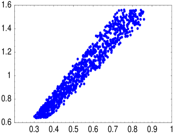
$Br({\tilde{\nu}}_{\tau}\to e\tau)/Br({\tilde{\nu}}_{\tau}\to\mu\tau)$

$Br({\tilde{\nu}}_{\tau}\to e\tau)/Br({\tilde{\nu}}_{\tau}\to\mu\tau)$

$(\epsilon_{1}/\epsilon_{2})^{2}$                                                $\tan^{2}\theta_{\odot}$

Figure 2: Ratio of branching ratios $Br({\tilde{\nu}}_{\tau}\to e\tau)/Br({\tilde{\nu}}_{\tau}\to\mu\tau)$ versus a) (left) $(\epsilon_{1}/\epsilon_{2})^{2}$ and b) (right) $\tan^{2}\theta_{\odot}$ for scenario I.

Tau sneutrinos, on the other hand, will decay to final states $e\tau$ and $\mu\tau$ with sizable branching ratios

$$\frac{Br({\tilde{\nu}}_{\tau}\rightarrow e\tau)[Br({\tilde{\nu}}_{\tau}\rightarrow\mu\tau)]}{Br({\tilde{\nu}}_{\tau}\rightarrow b{\bar{b}})}\simeq\frac{h^{2}_{\tau}}{3h^{2}_{b}(1+\Delta_{QCD})}\frac{\epsilon_{1}^{2}[\epsilon_{2}^{2}]}{\epsilon_{3}^{2}}$$ (32)

The above relation allows one to cross check the consistency of the bilinear scenario with neutrino data, as demonstrated in Fig. (2). The current $3\sigma$ allowed range for $\tan^{2}\theta_{\odot}$ of $\tan^{2}\theta_{\odot}=$ [$0.30,0.59$] fixes $Br({\tilde{\nu}}_{\tau}\rightarrow e\tau)/Br({\tilde{\nu}}_{\tau}\rightarrow\mu\tau)\simeq[0.55,1.25]$, as can be seen in Fig. (2).

Non-zero sneutrino vevs induce the decay ${\tilde{\nu}}\rightarrow\nu\nu$, i.e. by measuring non-zero branching ratios for invisible decays one could establish that sneutrino vevs exist. From the estimate on $\frac{v}{M_{2}}$ and $\frac{\epsilon}{\mu}$ discussed above one can estimate that branching ratios of sneutrino decays to invisible states should be of the order ${\cal O}(10^{-4})$.

Figure (3) shows the calculated branching ratios for invisible final states, $Br(\tilde{\nu}_{i}\to\sum\nu_{j}\nu_{k})$, as a function of the sneutrino mass. The figure shows that the estimate discussed above is correct within an order of magnitude. It also demonstrates that for sneutrinos below $m_{\tilde{\nu}}\leq 500$ GeV one expects $Br(\tilde{\nu}_{i}\to\sum\nu_{j}\nu_{k})\geq 10^{-5}$, i.e. with the cross sections calculated, see Fig. 1, a few events per year are expected with the signature $l^{+}l^{-}b{\bar{b}}$ + missing energy (from chargino pair production) and $b{\bar{b}}$ + missing energy (from sneutrino pair production).

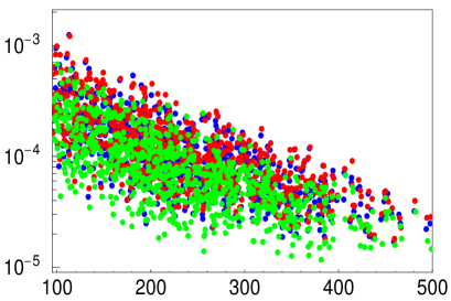
$Br(\tilde{\nu}_{i}\to\sum\nu_{j}\nu_{k})$

$m_{\tilde{\nu}}$ [GeV]

Figure 3: Invisible sneutrino decay branching ratio versus sneutrino mass for scenario I. Light (medium, dark) points (green, red, blue) are for ${\tilde{\nu}}_{e}$ (${\tilde{\nu}}_{\mu}$, ${\tilde{\nu}}_{\tau}$).

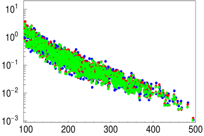
$L(\tilde{\nu}_{i})$ [$\mu m$]

$m_{\tilde{\nu}}$ [GeV]

Figure 4: Sneutrino decay length versus sneutrino mass for scenario I.

To measure absolute values of R-parity violating parameters it would be necessary to measure the decay widths of the sneutrinos. Given the current neutrino data, however, such a measurement seems to be out of reach for the next generation of colliders. Figure (4) shows calculated decay lengths, assuming a center of mass energy of $\sqrt{s}=1$ TeV, versus sneutrino mass. The decay lengths are short compared to sensitivities expected at a future linear collider which are of order 10 $\mu$m [34]. One can turn this argument around to conclude that observing decay lengths much larger than those shown in Fig. (4) would rule out explicit R-parity violation as the dominant source of neutrino mass.

4.2 Scenario II: $\lambda^{\prime}_{ijk}\simeq 0$

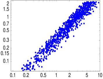
$\frac{Br({\tilde{\nu}}_{e}\to\tau\tau)/Br({\tilde{\nu}}_{\mu}\to\tau\tau)}{Br({\tilde{\nu}}_{e}\to\mu\mu)/Br({\tilde{\nu}}_{\mu}\to e\mu)}$

$(\lambda_{133}/\lambda_{233})^{2}$                                            $\tan^{2}\theta_{\odot}$

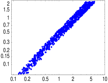
$\frac{Br({\tilde{\nu}}_{e}\to\tau\tau)/Br({\tilde{\nu}}_{\mu}\to\tau\tau)}{Br({\tilde{\nu}}_{e}\to\mu\mu)/Br({\tilde{\nu}}_{\mu}\to e\mu)}$

$(\lambda_{133}/\lambda_{233})^{2}$                                            $\tan^{2}\theta_{\odot}$

Figure 5: Double ratio of branching ratios $\frac{Br({\tilde{\nu}}_{e}\to\tau\tau)/Br({\tilde{\nu}}_{\mu}\to\tau\tau)}{Br({\tilde{\nu}}_{e}\to\mu\mu)/Br({\tilde{\nu}}_{\mu}\to e\mu)}$ as a function of a) (left) $(\lambda_{133}/\lambda_{233})^{2}$ and b) (right) $\tan^{2}\theta_{\odot}$ for scenario II. Top panel: All $\lambda_{ijk}$ same order of magnitude. Bottom panel: Assuming $\lambda_{133}$ and $\lambda_{233}$ larger than all other $\lambda_{ijk}$ by a factor of a few.

In this scenario we assume that the atmospheric neutrino mass scale is due to tree-level (bilinear) R-parity violation, while the solar neutrino mass scale is due to charged scalar loops ($\lambda_{ijk}$), assuming $\lambda^{\prime}_{ijk}\ll\lambda_{ijk}$. In this scenario the atmospheric neutrino data as well as $U^{2}_{e3}$ fix the allowed ranges for the $v_{i}$ whereas the solar neutrino data fix the ranges for $\lambda_{133}$ and $\lambda_{233}$.

We have calculated branching ratios for invisible sneutrino decays and find that they are smaller than for the bilinear-only case shown in Fig. (3), and thus not measurable. Also sneutrino decay lengths in this scenario are smaller than the ones shown in Fig. (4). From a phenomenological point of view this scenario mainly differs from the bilinear-only case in the fact that (by assumption) there are very few jets in the decays of sneutrinos.

Ratios of branching ratios can measure ratios of $\lambda_{ijk}$ and despite the fact that we assume here no hierarchy for the $\lambda_{ijk}$ this feature can be used to create a cross check of the scenario with solar neutrino physics. As an example we show in Fig. (5) double ratios of branching ratios as a function of $(\lambda_{133}/\lambda_{233})^{2}$ (left) and as a function of $\tan^{2}\theta_{\odot}$ (right). The correlation of this double ratio with $(\lambda_{133}/\lambda_{233})^{2}$ can be easily understood, since

$$Br({\tilde{\nu}}_{e}\to\tau\tau)\simeq c_{{\tilde{\nu}}_{e}}\lambda_{133}^{2} Br({\tilde{\nu}}_{\mu}\to\tau\tau)\simeq c_{{\tilde{\nu}}_{\mu}}\lambda_{233}^{2}$$ (33)

$$Br({\tilde{\nu}}_{e}\to\mu\mu)\simeq c_{{\tilde{\nu}}_{e}}\lambda_{122}^{2} Br({\tilde{\nu}}_{\mu}\to e\mu)\simeq c_{{\tilde{\nu}}_{\mu}}\lambda_{122}^{2}$$

where $c_{{\tilde{\nu}}_{\mu}}$ and $c_{{\tilde{\nu}}_{e}}$ are constants which differ for the different generations of sneutrinos but which cancel in the double ratio. Here we have considered two limiting scenarios (i) $|\lambda_{133}|$ and $|\lambda_{233}|$ are larger than the other $\lambda_{ijk}$ and (ii) all of them are in the same order of magnitude. Interestingly, Fig. (5) demonstrates that a correlation of $(\lambda_{133}/\lambda_{233})^{2}$ with the solar angle exists even if all $\lambda_{ijk}$ are of the same order of magnitude. Clearly, these two scenarios can easily be distinguished at future collider experiments as in the first scenario $\tilde{\nu}_{e}$ and $\tilde{\nu}_{\mu}$ decay mainly into taus and $\tilde{\nu}_{\tau}$ decays mainly in a $l^{\pm}\tau^{\pm}$ (l=$e,\mu$) whereas in the second scenario the variety of different decay channels is much larger for all sneutrinos.

4.3 Scenario III: $v_{i}\simeq 0$

In this scenario we assume that the neutrino mass matrix is dominated by trilinear terms and that the sneutrino vevs are negligible. There are thus no invisible decays of sneutrinos. We have checked that decay lengths in this scenario are even shorter than in scenario II.

Even for all $\lambda_{ijk}$ and $\lambda^{\prime}_{ijk}$ different from zero ratios of $\lambda_{ijk}$ (and $\lambda^{\prime}_{ijk}$) can be measured from double ratios of branching ratios as demonstrated in Fig. (6), left panel.

If one assumes in addition (the validity of this assumption can be checked by measuring branching ratios) that $\lambda_{i33}$ and $\lambda^{\prime}_{233}$ and $\lambda^{\prime}_{333}$ are somewhat larger than the other $\lambda_{ijk}$ and $\lambda^{\prime}_{ijk}$ one can make a consistency check with solar and atmospheric angle, as shown in Fig. (6), right panel. Note that the correlation with the solar angle will be lost if all $\lambda_{ijk}$ are of the same size and/or $\lambda^{\prime}_{ijk}$ with $j,k\neq 3$ are about equal to $\lambda_{i33}$ . Also the correlation with the atmospheric angle gets less pronounced if $\lambda^{\prime}_{133}$ approaches $\lambda^{\prime}_{333}$. However, the latter would be in contradiction to the observed smallness of the reactor angle and thus rule out one assumption of scenario III (atmospheric scale due to $\lambda^{\prime}_{ijk}$) as well.

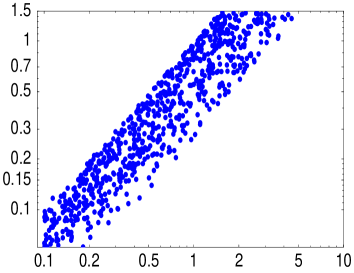
$\frac{Br({\tilde{\nu}}_{e}\to\tau\tau)/Br({\tilde{\nu}}_{\mu}\to\tau\tau)}{Br({\tilde{\nu}}_{e}\to\mu\mu)/Br({\tilde{\nu}}_{\mu}\to e\mu)}$

$(\lambda_{133}/\lambda_{233})^{2}$                                            $\tan^{2}\theta_{\odot}$

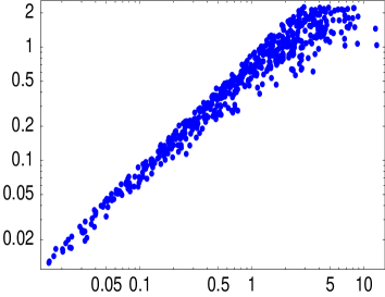
$\frac{Br({\tilde{\nu}}_{\mu}\to bb)/Br({\tilde{\nu}}_{\tau}\to bb)}{Br({\tilde{\nu}}_{\mu}\to\tau\tau)/Br({\tilde{\nu}}_{\tau}\to\mu\tau)}$

$(\lambda^{\prime}_{233}/\lambda^{\prime}_{333})^{2}$                                            $\tan^{2}\theta_{Atm}$

Figure 6: Top panel: Double ratio of branching ratios $\frac{Br({\tilde{\nu}}_{e}\to\tau\tau)/Br({\tilde{\nu}}_{\mu}\to\tau\tau)}{Br({\tilde{\nu}}_{e}\to\mu\mu)/Br({\tilde{\nu}}_{\mu}\to e\mu)}$ versus a) (left) $(\lambda_{133}/\lambda_{233})^{2}$ and b) (right) $\tan^{2}\theta_{\odot}$ for scenario III. Bottom panel: Double ratio of branching ratios $\frac{Br({\tilde{\nu}}_{\mu}\to bb)/Br({\tilde{\nu}}_{\tau}\to bb)}{Br({\tilde{\nu}}_{\mu}\to\tau\tau)/Br({\tilde{\nu}}_{\tau}\to\mu\tau)}$ versus a) (left) $(\lambda^{\prime}_{233}/\lambda^{\prime}_{333})^{2}$ and b) (right) $\tan^{2}\theta_{Atm}$. See text.

5 Conclusion

We have calculated the decay properties of sneutrinos assuming that they are the lightest supersymmetric particles in general R-parity violating models. The decay properties can be used to get information of the relative importance of bilinear R-parity breaking couplings versus trilinear R-parity breaking couplings which is quite interesting from the model building point of view. We have seen that in the case of bilinear dominance two important features occur: (i) the existence of the invisible decay mode $\tilde{\nu}_{i}\to\nu_{j}\nu_{k}$ with a branching ratio of the order $10^{-4}$ and (ii) the visible decay modes are governed by the lepton and down-quark Yukawa couplings with the dominant mode into $\bar{b}b$ followed by $\tau^{+}\tau^{-}$. In the case that trilinear terms become important both features are changed as we have shown.

Let us briefly comment on differences in the phenomenology between neutralino LSP, the most commonly studied LSP candidate, and sneutrino LSPs at future collider experiments such as LHC or a prospective ILC in scenarios where R-parity is broken by lepton number breaking terms. The most striking difference is that sneutrino LSPs decay nearly to 100% visible states with hardly any missing energy whereas the neutralino has several final states containing neutrinos. This implies that in the scenarios discussed here there are several decay chains relevant for LHC which do not contain any missing energy, e.g. $\tilde{q}_{L}\to q^{\prime}\tilde{\chi}^{\pm}_{1}\to q^{\prime}l^{\pm}\tilde{\nu}_{l}\to q^{\prime}l^{\pm}b\bar{b}$ which clearly affects the strategies to identify the particles as well as the determination of the underlying model parameters. However, decay chains containing a neutralino still lead to the missing energy signature in such cases due the the decay $\tilde{\chi}^{0}_{i}\to\nu\tilde{\nu}$, which, depending on the mass difference $m_{\tilde{\chi}^{0}_{i}}-m_{\tilde{\nu}}$, still can be sizable.

Moreover, we have shown that despite the large number of parameters certain ratios of branching ratios of sneutrino decays can be used to devise consistency checks with neutrino physics in all scenarios considered. To accomplish this we have proposed to flavour tack the sneutrinos in chargino decays as this substantially increases the possibilities to perform the cross check between observables in neutrino experiments and observables at future high energy collider experiments.

References

- [1] L. J. Hall and M. Suzuki, Nucl. Phys. B 231 (1984) 419.
- [2] J. C. Romao, C. A. Santos and J. W. F. Valle, Phys. Lett. B 288 (1992) 311; G. F. Giudice, A. Masiero, M. Pietroni and A. Riotto, Nucl. Phys. B 396 (1993) 243 [arXiv:hep-ph/9209296]. M. Hirsch, J. C. Romao, J. W. F. Valle and A. Villanova del Moral, arXiv:hep-ph/0407269.
- [3] B. C. Allanach, A. Dedes and H. K. Dreiner, Phys. Rev. D 69 (2004) 115002 [arXiv:hep-ph/0309196].
- [4] S. Eidelman et al. [Particle Data Group Collaboration], Phys. Lett. B 592 (2004) 1.
- [5] A. Brignole, L. E. Ibañez and C. Muñoz, Nucl. Phys. B 422 (1994) 125 [Erratum-ibid. B 436 (1995) 747] [arXiv:hep-ph/9308271]; A. Brignole, L. E. Ibanez, C. Munoz and C. Scheich, Z. Phys. C 74 (1997) 157 [arXiv:hep-ph/9508258].
- [6] C. F. Kolda and S. P. Martin, Phys. Rev. D 53 (1996) 3871 [arXiv:hep-ph/9503445].
- [7] B. Mukhopadhyaya, S. Roy and F. Vissani, Phys. Lett. B 443 (1998) 191 [arXiv:hep-ph/9808265]. A. Datta, B. Mukhopadhyaya and F. Vissani, Phys. Lett. B 492 (2000) 324 [arXiv:hep-ph/9910296].
- [8] W. Porod, M. Hirsch, J. Romao and J. W. F. Valle, Phys. Rev. D 63 (2001) 115004 [arXiv:hep-ph/0011248].
- [9] D. Restrepo, W. Porod and J. W. F. Valle, Phys. Rev. D 64 (2001) 055011 [arXiv:hep-ph/0104040].
- [10] M. Hirsch, W. Porod, J. C. Romao and J. W. F. Valle, Phys. Rev. D 66 (2002) 095006 [arXiv:hep-ph/0207334].
- [11] E. J. Chun, D. W. Jung, S. K. Kang and J. D. Park, Phys. Rev. D 66 (2002) 073003 [arXiv:hep-ph/0206030].
- [12] M. Hirsch and W. Porod, Phys. Rev. D 68 (2003) 115007 [arXiv:hep-ph/0307364].
- [13] A. Bartl, M. Hirsch, T. Kernreiter, W. Porod and J. W. F. Valle, JHEP 0311 (2003) 005 [arXiv:hep-ph/0306071].
- [14] D. W. Jung, S. K. Kang, J. D. Park and E. J. Chun, JHEP 0408 (2004) 017 [arXiv:hep-ph/0407106].
- [15] A. Heister et al. [ALEPH Collaboration], Eur. Phys. J. C 31 (2003) 1 [arXiv:hep-ex/0210014].
- [16] P. Achard et al. [L3 Collaboration], Phys. Lett. B 524 (2002) 65 [arXiv:hep-ex/0110057].
- [17] G. Abbiendi et al. [OPAL Collaboration], Eur. Phys. J. C 33 (2004) 149 [arXiv:hep-ex/0310054].
- [18] J. Abdallah et al. [DELPHI Collaboration], [arXiv:hep-ex/0406009].
- [19] J. Abdallah et al. [DELPHI Collaboration], Eur. Phys. J. C 28 (2003) 15 [arXiv:hep-ex/0303033].
- [20] S. Dimopoulos and L. J. Hall, Phys. Lett. B 207 (1988) 210.
- [21] V. D. Barger, G. F. Giudice and T. Han, Phys. Rev. D 40 (1989) 2987.
- [22] For a review on trilinear R-parity violation, see: H. K. Dreiner, hep-ph/9707435.
- [23] B. de Carlos and P. L. White, Phys. Rev. D55, 4222 (1997), [hep-ph/9609443]; B. de Carlos and P. L. White, Phys. Rev. D54, 3427 (1996), [hep-ph/9602381]; E. Nardi, Phys. Rev. D55, 5772 (1997), [hep-ph/9610540].
- [24] M. Hirsch, M. A. Diaz, W. Porod, J. C. Romao and J. W. F. Valle, Phys. Rev. D62, 113008 (2000), [hep-ph/0004115]; [Erratum-ibid. D 65 (2002) 119901];
- [25] M. A. Diaz, M. Hirsch, W. Porod, J. C. Romao and J. W. F. Valle, D68, 013009 (2003) hep-ph/0302021
- [26] H. K. Dreiner and M. Thormeier, Phys. Rev. D 69 (2004) 053002 [arXiv:hep-ph/0305270].
- [27] A. S. Joshipura and M. Nowakowski, Phys. Rev. D 51 (1995) 2421 [arXiv:hep-ph/9408224].
- [28] M. Hirsch and J. W. F. Valle, Nucl. Phys. B557, 60 (1999), [hep-ph/9812463].
- [29] F. Borzumati and J. S. Lee, Phys. Rev. D 66 (2002) 115012 [arXiv:hep-ph/0207184].
- [30] B. C. Allanach, C. G. Lester, M. A. Parker and B. R. Webber, JHEP 0009 (2000) 004 [arXiv:hep-ph/0007009].
- [31] S. Ambrosanio, G. D. Kribs and S. P. Martin, Nucl. Phys. B 516 (1998) 55 [arXiv:hep-ph/9710217].
- [32] A. Djouadi and Y. Mambrini, Phys. Rev. D 63 (2001) 115005 [arXiv:hep-ph/0011364].
- [33] M. Chaichian, A. Datta, K. Huitu, S. Roy and Z. h. Yu, Phys. Lett. B 594 (2004) 355 [arXiv:hep-ph/0311327].
- [34] T. Behnke, S. Bertolucci, R. D. Heuer and R. Settles, “TESLA: The superconducting electron positron linear collider with an integrated X-ray laser laboratory. Technical design report. Pt. 4: A detector for TESLA,” DESY-01-011