IISc-CHEP-12/04

1. Introduction

Early work on the scalar form factors of the pion [1, 2] was motivated by the search for a very light Higgs particle. Unfortunately, the outcome of this search was negative: nature is kind enough to let us probe the vector and axial currents, but allows us to experimentally explore only those scalar and pseudoscalar currents that are connected with flavour symmetry breaking. In particular, there is no handle on the matrix element

$$\Gamma_{\pi}(t)=\langle\pi(p^{\prime})|m_{u}\,\overline{\rule[4.19998pt]{3.99994pt}{0.0pt}}uu+m_{d}\,\,\overline{\rule[6.49994pt]{3.99994pt}{0.0pt}}dd|\pi(p)\rangle\,,\hskip 20.00003ptt=(p^{\prime}-p)^{2}\,.$$ (1)

The value of this form factor at $t=0$ is referred to as the pion $\sigma$-term,

$$\Gamma_{\pi}(0) \!\!\!= \!\!\!m_{u}\,\frac{\partial M_{\pi}^{2}}{\partial m_{u}}+m_{d}\,\frac{\partial M_{\pi}^{2}}{\partial m_{d}}\,.$$ (2)

According to Gell-Mann, Oakes and Renner [3], the expansion of the square of the pion mass starts with a term linear in $m_{u}$ and $m_{d}$, the coefficient being determined by the quark condensate. Hence the pion $\sigma$-term is determined by the pion mass, except for corrections of higher order: $\Gamma_{\pi}(0)=M_{\pi}^{2}+O(\hat{m}^{2})$, with $\hat{m}=\frac{1}{2}(m_{u}+m_{d})$. Indeed, both the precision measurements on $K_{\ell 4}$ decay [4] and the preliminary results from DIRAC [5] confirm that the corrections are small: more than 94 % of the pion mass originates in the term generated by the quark condensate [6].

The scalar radius represents the slope of the corresponding normalized form factor $\bar{\Gamma}_{\pi}(t)\equiv\Gamma_{\pi}(t)/\Gamma_{\pi}(0)$,

$$\bar{\Gamma}_{\pi}(t)=1+\frac{1}{6}\langle r^{2}\rangle\rule[-1.99997pt]{0.0pt}{0.0pt}_{s}^{\pi}\,t+O(t^{2})\,,$$ (3)

which is of considerable interest, because it is related to the effective coupling constant $\bar{\ell}_{4}$, that determines the first nonleading contribution in the chiral expansion of the pion decay constant. Denoting the value of $F_{\pi}$ in the limit $m_{u}=m_{d}=0$ by $F$, we have [7]

$$\frac{F_{\pi}}{F}=1+\frac{1}{6}\,M_{\pi}^{2}\langle r^{2}\rangle\rule[-1.99997pt]{0.0pt}{0.0pt}_{s}^{\pi}+\frac{13M_{\pi}^{2}}{192\,\pi^{2}F_{\pi}^{2}}+O(\hat{m}^{2})\,.$$ (4)

There is a formula analogous to (4) also for $F_{K}/F_{\pi}$. Neglecting Zweig rule violating contributions and using the measured value of $F_{K}/F_{\pi}$, this relation leads to a first crude estimate for the scalar radius: $\langle r^{2}\rangle\rule[-1.99997pt]{0.0pt}{0.0pt}_{s}^{\pi}=0.55\pm 0.15\,\mbox{fm}^{2}$ [8]. An improved estimate was obtained long ago on the basis of dispersion theory [2]. The calculation relied on the assumption that only the transition $\pi\pi\rightarrow K\bar{K}$ generates inelasticity at low energies – all other inelastic channels in the Mushkhelishvili-Omnès (M-O) representation of the form factor were neglected. Moussallam [9] performed a thorough analysis of this approach, considering several different phase shift representations (in particular also the parametrizations proposed in [10]) and studying the sensitivity of the outcome to other inelastic reactions, such as $\pi\pi\rightarrow 4\pi$, $\pi\pi\rightarrow\eta\eta$. His results for the scalar radius are in the range from $0.58$ to $0.65\,\mbox{fm}^{2}$. In [11], the Roy equations for $\pi\pi$ scattering were used to update the calculation described in [2], with the result

$$\langle r^{2}\rangle\rule[-1.99997pt]{0.0pt}{0.0pt}_{s}^{\pi}=0.61\pm 0.04\,\mbox{fm}^{2}\,.$$ (5)

The central value confirms the number $\Gamma^{\prime}_{\pi}(0)/\Gamma_{\pi}(0)=2.6\,\mbox{GeV}^{-2}$ given in [2] and the error bar covers the range found by Moussallam.

The higher orders of the chiral perturbation series for the form factor $\Gamma_{\pi}(t)$ are discussed in [12] and a detailed comparison with the dispersive representation can also be found there. The complete evaluation to two loops is given in [13]. The corrections of $O(\hat{m}^{2})$ in the relation (4) are discussed in [14]. With the estimates for the higher order terms given in [15], we obtain $F_{\pi}/F=1.072\pm 0.004$. As the corrections are (a) very small and (b) dominated by known double logarithms, the uncertainty in the result is due almost exclusively to the one in the scalar radius.

The effective couplings relevant for the masses and decay constants can be measured on the lattice [16]. Using the values for $L_{4}$, $L_{5}$, $L_{6}$ and $L_{8}$ found by the MILC collaboration [17], the corresponding values of the SU(2)$\times$SU(2) coupling constants are readily worked out from the relations given in [18]. This leads to $\bar{\ell}_{3}=0.8\pm 2.3$, $\bar{\ell}_{4}=4.0\pm 0.6$, in good agreement with the estimates given 20 years ago. Inserting this value for $\bar{\ell}_{4}$ in the relevant one loop formulae, we obtain $F_{\pi}/F=1.06\pm 0.01$, $\langle r^{2}\rangle\rule[-1.99997pt]{0.0pt}{0.0pt}_{s}^{\pi}=0.5\pm 0.1\,\mbox{fm}^{2}$. A direct determination of the ratio $F_{\pi}/F$ on the lattice would be of considerable interest.

2. Omnès representation

Ynduráin’s paper on the subject [19] is based on the Omnès representation,

$$\bar{\Gamma}_{\pi}(t)=\exp\frac{t}{\pi}\int_{4M_{\pi}^{2}}^{\infty}\frac{ds\,\delta_{\hskip 0.35002pt\Gamma}(s)}{s\,(s-t)}\,,$$ (6)

which expresses the form factor in terms of its phase on the upper rim of the cut, $\delta_{\hskip 0.35002pt\Gamma}(s)=\arg\Gamma_{\pi}(s+i\,\epsilon)$. The formula may be viewed as a one-channel version of the M-O representation (in that framework, the absence of inelastic channels implies that the phase of the form factor coincides with the phase of the scattering amplitude). Perturbative QCD indicates that the form factor behaves asymptotically as $|\Gamma_{\pi}(t)|\sim 1/|t|$ up to logarithms [20]. If the form factor does not have zeros, the phase $\delta_{\hskip 0.35002pt\Gamma}(s)$ must tend to $\pi$. The formula (6) then rigorously holds and leads to a rapidly convergent representation for the scalar radius,

$$\langle r^{2}\rangle\rule[-1.99997pt]{0.0pt}{0.0pt}_{s}^{\pi}=\frac{6}{\pi}\int_{4M_{\pi}^{2}}^{\infty}\frac{ds\,\delta_{\hskip 0.35002pt\Gamma}(s)}{s^{2}}\,.$$ (7)

Unless the asymptotics is assumed to set in at an unreasonably low energy, the corrections from the preasymptotic logarithms are negligibly small.

The Watson theorem states that, in the elastic region, the phase of the form factor coincides with the isoscalar S-wave $\pi\pi$ phase shift, $\delta_{\hskip 0.35002pt\Gamma}=\delta_{0}^{0}$. Below the $K\bar{K}$ threshold, inelastic processes do not play a significant role: on the interval $4M_{\pi}^{2}<s<4M_{K}^{2}$, the elasticity $\eta_{0}^{0}$ remains very close to 1, so that $\delta_{\hskip 0.35002pt\Gamma}$ remains close to $\delta_{0}^{0}$. With the representation for the phase $\delta_{0}^{0}$ obtained in ref. [11], the contribution from that interval can be evaluated quite accurately.

The opening of the $K\bar{K}$ channel produces a square root singularity at $4M_{K}^{2}$, which manifests itself as a dip in the elasticity in the region between 1 and 1.1 GeV. Although the valley may not be very deep, there is no reason for the phase of the form factor to agree with $\delta_{0}^{0}$ in that region. Various models have been proposed to account for the fact that the Omnès factor belonging to $\delta_{0}^{0}$ does not properly describe the behaviour of the form factor $\Gamma_{\pi}(t)$ or of other transition amplitudes involving the production of pion pairs (see for instance [21, 22, 23, 24]).

Ynduráin assumes that the perturbative asymptotics sets in at 1.42 GeV, observes that in the region between 1.1 and 1.42 GeV, the inelasticity is compatible with zero and then claims: It thus follows that the phase of $\Gamma_{\pi}(s)$ must be approximately equal to $\delta_{0}^{0}(s)$ for $1.1\,\mbox{GeV}<s^{1/2}<1.42\,\mbox{GeV}$. This claim is incorrect, for the following reason: in the presence of inelastic channels, the Watson theorem in general reads

$$\Gamma_{m}^{\star}(s)=\sum_{n}\,\{\delta_{mn}+2\,i\,T_{mn}(s)\,\sigma_{n}(s)\}^{\star}\,\Gamma_{n}(s)\,.$$ (8)

We use the notation of [2] and identify the first two channels with $\pi\pi$ and $K\bar{K}$:

$$\Gamma_{1}(s)=\Gamma_{\pi}(s)\,,\;\;\Gamma_{2}(s)=\frac{2}{\sqrt{3}}\,\Gamma_{K}(s)\,,\;\;\sigma_{1}(s)=\sigma_{\pi}(s)\,,\;\;\sigma_{2}(s)=\sigma_{K}(s)\,,$$ (9)

with $\sigma_{P}(s)\equiv\theta(s-4M_{P}^{2})(1-4M_{P}^{2}/s)^{1/2}$. The term $T_{11}$ stands for the partial wave amplitude of the isoscalar $S$-wave,

$$T_{11}\equiv t_{0}^{0}=\frac{\eta_{0}^{0}\exp(2\,i\,\delta_{0}^{0})-1}{2i\sigma_{\pi}}\,.$$ (10)

If all other channels are ignored, unitarity fixes the magnitude of $T_{12}$ above the $K\bar{K}$ threshold in terms of the elasticity: $4\,\sigma_{1}\sigma_{2}\,|T_{12}|^{2}=1-(\eta_{0}^{0})^{2}$. For energies where $\eta_{0}^{0}\simeq 1$, the condition (8) thus reduces to $\Gamma_{\pi}^{\star}\simeq\exp(-2\,i\delta_{0}^{0})\,\Gamma_{\pi}.$ This relation does not imply that the difference $\delta_{\hskip 0.35002pt\Gamma}-\delta_{0}^{0}$ approximately vanishes, but only requires that it is close to a multiple of $\pi$.

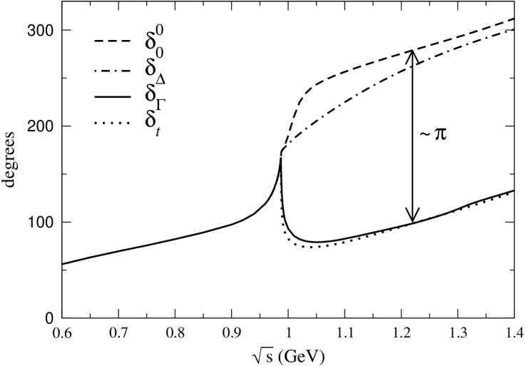
Figure 1: The full line is the phase of the pion form factor of the operators $\bar{u}u$ or $\bar{d}d$, as calculated from the two-channel M-O equations. The dashed and dotted lines describe the corresponding phase shift and the phase of the partial wave amplitude, respectively. The dash-dotted line depicts the phase of the form factor belonging to the operator $\bar{s}s$.

One might think that continuity would remove the ambiguity, but this is not the case, because the region of interest is separated from the elastic domain by an interval were inelasticity cannot be ignored. The full line in fig. 1 depicts the outcome of our calculation for the phase of the form factor: above 1.1 GeV, $\delta_{\hskip 0.35002pt\Gamma}$ indeed differs from $\delta_{0}^{0}$, approximately by $\pi$. The detailed behaviour in the region around 1 GeV is sensitive to the properties of the $T$-matrix, but the entire range of representations considered in ref. [9] leads to a sharp drop of $\delta_{\hskip 0.35002pt\Gamma}$ at the $K\bar{K}$ threshold and to $\delta_{0}^{0}-\delta_{\hskip 0.35002pt\Gamma}\simeq\pi$ for energies above 1.1 GeV [26]. In other words, the robust lower bound in [19] is not valid, because it is derived from an incorrect claim.

The dotted line in the figure depicts the phase of the partial wave amplitude, $\delta_{t}=\mbox{arg}\,t_{0}^{0}$ – the phase of the form factor closely follows this line. The explicit calculation based on two-channel unitarity thus leads to a behaviour of the scalar form factor of the type proposed by Morgan and Pennington for the diffractive production of $\pi\pi$ final states [21]. Indeed, fig. 2 in their paper on the reaction $p\,p\rightarrow p\,p\,\pi\,\pi$ [27] is closely related to ours: it shows the result of the energy independent analysis of the Hyams data for $\delta_{0}^{0}$ and $\delta_{t}$, while, above $4M_{K}^{2}$, the dotted and dashed curves in our plot represent the result of the energy dependent analysis of the same data.

3. Importance of inelastic channels

The reason for the pronounced difference between $\delta_{0}^{0}$ and $\delta_{t}$ is readily understood from the Argand diagram: As the energy reaches $2M_{K}$, the amplitude has nearly completed a full circle. If inelasticity could be ignored, the curve would continue following the Argand circle, so that $t_{0}^{0}$ would have a zero, a few MeV above the $K\bar{K}$ threshold. Hence the phase $\delta_{t}$ would make a jump there, dropping abruptly by $\pi$. In reality, the curve leaves the circle before the phase has reached $\pi$, so that $t_{0}^{0}$ remains different from zero and a jump does not occur. Instead, $\delta_{0}^{0}-\delta_{t}$ continuously, but rapidly grows from 0 to the vicinity of $\pi$.

The phenomenon illustrates the fact that phases of small quantities can be very sensitive to details. The phase of $t_{0}^{0}$ undergoes a dramatic change because it so happens that an inelastic channel opens up at an energy where $t_{0}^{0}$ nearly vanishes. The magnitude of the change in $\delta_{0}^{0}-\delta_{\hskip 0.35002pt\Gamma}$ is by no means proportional to the probability for the formation of a $K\bar{K}$ pair, i.e. to the inelasticity $1-(\eta_{0}^{0})^{2}$, but is approximately equal to $\pi$. If the inelasticity is small, the change in the phase difference takes place almost instantly.

In connection with the Omnès formula, the difference between the phase shift and the phase of the partial wave is a measure of the importance of inelastic channels. Above 1.1 GeV, both $\delta_{\hskip 0.35002pt\Gamma}\simeq\delta_{0}^{0}$ and $\delta_{\hskip 0.35002pt\Gamma}\simeq\delta_{t}$ obey the Watson theorem. Fig. 2 shows that in the region below 1.4 GeV, an evaluation of the integral relevant for the scalar radius based on $\delta_{\hskip 0.35002pt\Gamma}\simeq\delta_{t}$ practically reproduces the result of our two-channel calculation, while using $\delta_{\hskip 0.35002pt\Gamma}\simeq\delta_{0}^{0}$ leads to values like those advocated in [19], which are significantly higher. So, inelastic reactions are important here: In order to determine the scalar radius, we need to know their impact on the form factor.

For the electromagnetic form factor of the pion, the situation is qualitatively different. In that case, inelastic channels play a much less important role. In particular, the angular momentum barrier suppresses the branch point singularity connected with the opening of the $K\bar{K}$ channel. Since the $P$-wave phase shift $\delta_{1}^{1}$ stays well below $180^{\circ}$, the partial wave amplitude $t_{1}^{1}$ does not become small there, so that the phenomenon observed in the $S$-wave does not occur: the difference between $\delta_{1}^{1}$ and the phase of $t_{1}^{1}$ grows much more slowly than in that case: at 1.1 GeV, it amounts to a few degrees, while $\delta_{0}^{0}-\delta_{t}\simeq 180^{\circ}$. In this connection, we recall that, for the case of the electromagnetic form factor, Eidelman and Lukaszuk [28] have shown that the experimental information on $e^{+}e^{-}$ production of final states other than $\pi\pi$ implies rather stringent bounds on the elasticity $\eta_{1}^{1}$ and on the difference between the phase shift $\delta_{1}^{1}$ and the phase of the form factor.

The behaviour of the form factor at the onset of the $K\bar{K}$ continuum reflects the strength of the coupling to these states. For the operator $\hskip 1.99997pt\overline{\rule[4.19998pt]{3.99994pt}{0.0pt}}s\hskip 1.00006pts$, this coupling differs from $\overline{\rule[4.19998pt]{3.99994pt}{0.0pt}}uu$ or $\,\overline{\rule[6.49994pt]{3.99994pt}{0.0pt}}dd$. Hence we should expect that the phase $\delta_{\Delta}(s)=\mbox{arg}\,\Delta_{\pi}(s+i\,\epsilon)$ of the form factor

$$\Delta_{\pi}(t)=\langle\pi(p^{\prime})|\,m_{s}\hskip 1.99997pt\overline{\rule[4.19998pt]{3.99994pt}{0.0pt}}s\hskip 1.00006pts|\pi(p)\rangle$$ (11)

behaves quite differently from $\delta_{\hskip 0.35002pt\Gamma}(s)$. As shown in [2], $\Delta_{\pi}(t)$ is given by a different linear combination of the same two linearly independent solutions of the M-O equations that are needed for the evaluation of $\Gamma_{\pi}(t)$. In fig. 1, the phase of the resulting representation of the form factor is shown as a dash-dotted line. The figure shows that $\delta_{\Delta}$ roughly follows the phase shift $\delta_{0}^{0}$: above the $K\bar{K}$ threshold, the phases of the two form factors are very different.

4. Magnitude of the form factors

Fig. 2 shows the magnitude of the Omnès factors obtained by inserting the phases depicted in fig. 1 in the formula (6). The full curve represents our result for the form factor $|\bar{\Gamma}_{\pi}(s)|$ and shows that this quantity exhibits a dip at the $K\bar{K}$ threshold – the phenomenon discussed by Morgan and Pennington. Indeed, the figure shows that the result for this form factor is very close to the Omnès factor belonging to the phase $\delta_{t}$. Moussallam’s analysis confirms the phenomenon: for all of the $T$-matrix representations considered in [9], the function $|\Gamma_{\pi}(s)|$ goes through a sharp minimum near the $K\bar{K}$ threshold [26].

The minimum reflects the rapid drop in the phase: the Omnès factor belonging to the phase $\delta(s)=\theta(s-4M_{K}^{2})\,(-\pi)$ is given by $1-t/4M_{K}^{2}$. In other words, if the phase were to drop suddenly by $\pi$ at $s=4M_{K}^{2}$, then the corresponding Omnès factor would contain a zero there. In reality, the phase does not drop suddenly, but rapidly – the magnitude of the form factor does not go through a zero, but through a minimum. Conversely, the fact that the form factor becomes very small near the $K\bar{K}$ threshold implies that the behaviour of its phase there is very sensitive to details and cannot be understood without explicitly accounting for the $K\bar{K}$ channel.

For $\delta_{\Delta}$, on the other hand, the Omnès factor exhibits a peak near the $K\bar{K}$ threshold. Below 1 GeV, the behaviour is very similar to the one of the Omnès factor evaluated with $\delta_{0}^{0}$: if (as advocated by Ynduráin) the phase of $\Gamma_{\pi}$ were to follow $\delta_{0}^{0}$ rather than $\delta_{t}$, this form factor would exhibit a pronounced peak rather than a dip. This reflects the fact that the operator $\hskip 1.99997pt\overline{\rule[4.19998pt]{3.99994pt}{0.0pt}}s\hskip 1.00006pts$ couples more strongly to the kaon than to the pion. Near $t=0$, the difference is not enormous, but the slope is of course larger: evaluating the integral in (5) with $\delta_{\Delta}$ instead of $\delta_{\Gamma}$, we obtain $0.81\,\mbox{fm}^{2}$, instead of the number $0.61\pm 0.04\,\mbox{fm}^{2}$ quoted above. The behaviour of $\delta_{\Delta}$ near the $K\bar{K}$ threshold is subject to considerable uncertainties – we did not make an attempt at estimating those in the corresponding radius.

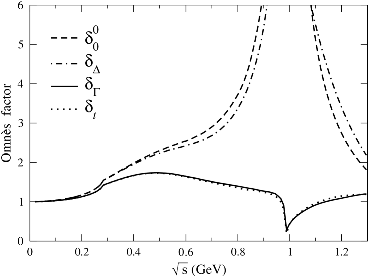
Figure 2: Omnès factors belonging to the phases shown in fig. 1.

There is a qualitative difference between the two form factors under consideration here: our representation for $\Delta_{\pi}(t)$ has a zero, but $\Gamma_{\pi}(t)$ does not. The reason is that $\Delta_{\pi}(0)$ represents the derivative of $M_{\pi}^{2}$ with respect to $m_{s}$ and hence vanishes for $m_{u}=m_{d}=0$, while the slope $\Delta^{\prime}_{\pi}(0)$ does not disappear in that limit. Accordingly, the Omnès representation involves a polynomial:

$$\Delta_{\pi}(t)=(p_{0}+p_{1}\,t)\,\exp\frac{t}{\pi}\int_{4M_{\pi}^{2}}^{\infty}\frac{ds\,\delta_{\Delta}(s)}{s\,(s-t)}\,.$$ (12)

The explicit representation in $\chi$PT to one loop [8] shows that $p_{0}$ is of $O(\hat{m})$, while $p_{1}$ is of $O(1)$ (the representation exclusively involves the Zweig rule violating constants $L_{4}$ and $L_{6}$). This demonstrates that the form factor $\Delta_{\pi}(t)$ necessarily has a zero at a value of $t$ of order $\hat{m}$, i.e. in the region where $\chi$PT is reliable. In order for the representation (12) to be consistent with perturbative asymptotics, the phase $\delta_{\Delta}$ must tend to $2\pi$ (compare fig. 1). Note that the dash-dotted curve in fig. 2 represents the magnitude of the exponential and does not account for the polynomial.

5. Scalar radius relevant for $K_{\ell 3}$ decay

The scalar form factor relevant for the decay $K\rightarrow\pi\ell\nu$ is proportional to the matrix element $\langle K|\hskip 1.99997pt\overline{\rule[4.19998pt]{3.99994pt}{0.0pt}}s\hskip 1.00006ptu|\pi\rangle$. We denote this form factor by $f_{0}(t)$, using the standard normalization, where the value at $t=0$ coincides with $f_{+}(0)$, a quantity that is of central importance for the determination of the CKM matrix element $V_{us}$. The term linear in $t$,

$$f_{0}(t)=f_{+}(0)\left\{1+\frac{1}{6}\,\langle r^{2}\rangle\rule[-1.99997pt]{0.0pt}{0.0pt}_{s}^{K\pi}\,t+c_{0}\,t^{2}+\ldots\right\}\,,$$ (13)

represents an analogue of the scalar radius of the pion. In the analysis of the data, it is customary to replace this radius by the slope parameter $\lambda_{0}\equiv\langle r^{2}\rangle\rule[-1.99997pt]{0.0pt}{0.0pt}_{s}^{K\pi}M_{\pi}^{2}/6$.

Nearly 20 years ago, a prediction for the radius was made, on the basis of $\chi$PT to one loop: $\langle r^{2}\rangle\rule[-1.99997pt]{0.0pt}{0.0pt}_{s}^{K\pi}=0.20\pm 0.05\,\mbox{fm}^{2}$ [8]. This number is about 3 times smaller than the scalar radius of the pion, an illustration of the fact that the scalar radii are very sensitive to flavour symmetry breaking – in contrast to the vector radii, where the flavour asymmetries are comparatively small. The corrections to the Callan-Treiman relation were also analyzed. In the formulation of Dashen and Weinstein, this relation represents a low energy theorem [29], which states that in the limit $m_{u}=m_{d}=0$, the value of $f_{0}(t)$ at $t=M_{K}^{2}-M_{\pi}^{2}$ coincides with the ratio $F_{K}/F_{\pi}$. As it turns out that the corrections of $O(\hat{m})$ do not contain a chiral logarithm of the type $M_{\pi}^{2}\log M_{\pi}^{2}$, they are tiny [8].

The experimental situation was not clear at that time: The outcome of a high statistics experiment [30] was in agreement with the theoretical expectations, but as explicitly stated in [8], the values for $\langle r^{2}\rangle\rule[-1.99997pt]{0.0pt}{0.0pt}_{s}^{K\pi}$ found in some of the more recent experiments cannot be reconciled with chiral symmetry. In the analysis of the Particle Data Group, the unsatisfactory experimental situation manifests itself in the fact that (a) the scale factors $S$ needed to account for the inconsistencies are large and (b) despite the stretching of error bars, the value found from decays of neutral kaons does not agree with the one from $K^{\pm}$ decay.

In this field, there was considerable progress recently, on the experimental as well as on the theoretical side. In particular, the $K_{\ell 3}$ form factors are now known to two loops of $\chi$PT [31, 32]. The curvature of the form factors cannot be neglected at the precision reached now and, in principle, a precise experimental determination thereof would allow a parameter free measurement of $V_{us}$ [32]. Moreover, Jamin, Oller and Pich observed that the curvature of the scalar form factor can be determined rather accurately by means of dispersive methods [33]. This implies that the radius can be calculated from the value of $f_{0}(t)$ at the Callan-Treiman point, $t=M_{K}^{2}-M_{\pi}^{2}$, for which $\chi$PT makes a very accurate prediction. In this way, the authors arrive at

$$\langle r^{2}\rangle\rule[-1.99997pt]{0.0pt}{0.0pt}_{s}^{K\pi}=0.192\pm 0.012\,\mbox{fm}^{2}\;\cite[cite]{[\@@bibref{}{Jamin Oller Pich 2004}{}{}]}\,.$$ (14)

The central value confirms the old result mentioned above, the uncertainty is four times smaller.

In [19], Ynduráin states that the value of $\lambda_{0}$ for charged kaon decay published by the PDG in 2000 is difficult to believe. Discarding the data prior to 1975, he arrives at $\langle r^{2}\rangle\rule[-1.99997pt]{0.0pt}{0.0pt}_{s}^{K\pi}=0.312\pm 0.070\,\mbox{fm}^{2}$ and concludes that the central value lies clearly outside the error bars of the chiral theory prediction. Indeed, if his central value was close to reality, we would have to conclude that experiment is in flat contradiction with a low energy theorem of SU(2)$\times$SU(2).

This is not the case, however. For the charged kaons, the data collected at the ISTRA detector clarified the situation considerably [34]. The result for the radius reads $\langle r^{2}\rangle\rule[-1.99997pt]{0.0pt}{0.0pt}_{s}^{K^{\pm}\pi}=0.235\pm 0.014\pm 0.007\,\mbox{fm}^{2}$ (note that in this case the radius is calculated from $\lambda_{0}$ using $M_{\pi^{0}}$) , which now dominates the world average. For the neutral kaons, the experimental situation also improved significantly: there is a new result from KTeV, $\langle r^{2}\rangle\mbox{\raisebox{-3.00003pt}{$\stackrel{{\scriptstyle K_{L}\pi}}{{\mbox{\footnotesize\it s}}}$}}=0.165\pm 0.016\,\mbox{fm}^{2}$ [35]. Since this value (a) now dominates the statistics and (b) is consistent with the 1974 high statistics experiment mentioned above, we conclude that there is a problem with those of the earlier data that were in conflict with chiral symmetry. While the value obtained from $K^{\pm}$ decay is higher than the prediction (14) by $2.1\,\sigma$, the KTeV result is lower by $1.4\,\sigma$. Chiral symmetry indicates that the truth is in the middle.

8. Conclusion

1. The low energy properties of the scalar pion form factors are governed by those of the isoscalar $S$-wave in $\pi\pi$ scattering. In particular, the reaction $\pi\pi\rightarrow K\bar{K}$ generates a pronounced structure in the vicinity of $s=4M_{K}^{2}$, which can be understood on the basis of a dispersive two-channel analysis. This framework leads to the conclusion that, in the region around 1 GeV, the pion matrix elements of $\overline{\rule[4.19998pt]{3.99994pt}{0.0pt}}uu$ and $\,\overline{\rule[6.49994pt]{3.99994pt}{0.0pt}}dd$ roughly follow the $\pi\pi$ partial wave amplitude $t_{0}^{0}$ and thus exhibit a sharp minimum there. The coupling of the operator $\hskip 1.99997pt\overline{\rule[4.19998pt]{3.99994pt}{0.0pt}}s\hskip 1.00006pts$ to the $K\bar{K}$ states differs from the one of $\overline{\rule[4.19998pt]{3.99994pt}{0.0pt}}uu$ or $\,\overline{\rule[6.49994pt]{3.99994pt}{0.0pt}}dd$. The corresponding form factor exhibits a pronounced peak rather than a dip.

2. The dispersive analysis leads to a rather accurate determination of the scalar radius of the pion. The early estimate given in [2] is confirmed. In particular, as shown in [9], the uncertainties in the phenomenological information used above 0.8 GeV do not significantly affect the result, which is in the range $\langle r^{2}\rangle\rule[-1.99997pt]{0.0pt}{0.0pt}_{s}=0.61\pm 0.04\,\mbox{fm}^{2}$ [11]. We draw attention to the fact that the two-loop prediction for the dependence of the pion decay constant on the mass of the two lightest quarks [14] can be used to convert determinations of $F_{\pi}$ on the lattice into a measurement of the scalar radius. The existing lattice data are consistent with the result of the dispersive calculation.

3. We discuss the impact of the new precision data on the scalar form factor of $K_{\ell 3}$ decay [34, 35]. Chiral symmetry leads to a low energy theorem for the value of this form factor at $t=M_{K}^{2}-M_{\pi}^{2}$. The new results, which now dominate the statistics, show that there is a problem with those of the old data that were in conflict with this prediction. Combining $\chi$PT to two loops [31, 32] with a dispersive analysis of the curvature, the low energy theorem can be converted into a very sharp prediction for the radius $\langle r^{2}\rangle\rule[-1.99997pt]{0.0pt}{0.0pt}_{s}^{K\pi}$ or for the slope parameter $\lambda_{0}$ [33]. Unfortunately, in view of the very small errors quoted for the slope, the new data on $K_{L}$ decay are not in agreement with those on $K^{\pm}$ decay: while the former are lower than the prediction, the latter are higher. Hopefully, the analysis of the data collected by the KLOE collaboration at Frascati [36] and by NA48 at CERN [37] will clarify the situation.

4. Ynduráin [19] states that the two-channel analysis in [2] is of the “black-box” type and claims that it is not necessary, that the phase of the form factor must approximately follow the phase shift $\delta_{0}^{0}$, that the scalar radius of the pion is subject to a lower bound and that the chiral theory prediction for $\langle r^{2}\rangle\rule[-1.99997pt]{0.0pt}{0.0pt}_{s}^{K\pi}$ disagrees with experiment. We have shown that none of these claims is tenable.

References

- [1] T. N. Truong and R. S. Willey, Phys. Rev. D 40 (1989) 3635.
- [2] J. F. Donoghue, J. Gasser and H. Leutwyler, Nucl. Phys. B 343, 341 (1990).
- [3] M. Gell-Mann, R. J. Oakes and B. Renner, Phys. Rev. 175 (1968) 2195.
- [4] S. Pislak et al. [BNL-E865 Collaboration], Phys. Rev. Lett. 87 (2001) 221801 [arXiv:hep-ex/0106071]; Phys. Rev. D 67 (2003) 072004 [arXiv:hep-ex/0301040].
- [5] L. Tauscher, talk given at DAFNE 2004: Physics at meson factories, 7-11 June 2004, Laboratori Nazionali di Frascati, Italy [http://www.lnf.infn.it/conference/dafne04/].
- [6] G. Colangelo, J. Gasser and H. Leutwyler, Phys. Rev. Lett. 86 (2001) 5008 [arXiv:hep-ph/0103063].
- [7] J. Gasser and H. Leutwyler, Phys. Lett. B 125 (1983) 325.
- [8] J. Gasser and H. Leutwyler, Nucl. Phys. B 250, 517 (1985).
- [9] B. Moussallam, Eur. Phys. J. C 14 (2000) 111 [arXiv:hep-ph/9909292].
- [10] R. Kaminski, L. Lesniak and B. Loiseau, Phys. Lett. B 413 (1997) 130 [arXiv:hep-ph/9707377]; Eur. Phys. J. C 9 (1999) 141 [arXiv:hep-ph/9810386]; Phys. Lett. B 551 (2003) 241 [arXiv:hep-ph/0210334].
- [11] G. Colangelo, J. Gasser and H. Leutwyler, Nucl. Phys. B 603 (2001) 125 [arXiv:hep-ph/0103088].
- [12] J. Gasser and U. G. Meissner, Nucl. Phys. B 357 (1991) 90.
- [13] J. Bijnens, G. Colangelo and P. Talavera, JHEP 9805, 014 (1998) [arXiv:hep-ph/9805389].
- [14] G. Colangelo, Phys. Lett. B 350, 85 (1995) [Erratum-ibid. B 361, 234 (1995)] [arXiv:hep-ph/9502285]; J. Bijnens, G. Colangelo, G. Ecker, J. Gasser and M. E. Sainio, Nucl. Phys. B 508 (1997) 263 [Erratum-ibid. B 517 (1998) 639] [arXiv:hep-ph/9707291].
- [15] G. Colangelo and S. Dürr, Eur. Phys. J. C 33 (2004) 543 [arXiv:hep-lat/0311023].
-
[16]
S. Dürr,
Eur. Phys. J. C 29 (2003) 383
[arXiv:hep-lat/0208051];
H. Wittig, Nucl. Phys. Proc. Suppl. 119 (2003) 59 [arXiv:hep-lat/0210025];
D. R. Nelson, G. T. Fleming and G. W. Kilcup, Phys. Rev. Lett. 90 (2003) 021601 [arXiv:hep-lat/0112029];
F. Farchioni, I. Montvay and E. Scholz [qq+q Collaboration], arXiv:hep-lat/0403014. - [17] C. Aubin et al. [MILC Collaboration], arXiv:hep-lat/0407028.
- [18] J. Gasser and H. Leutwyler, Nucl. Phys. B 250 (1985) 465, eq. (11.6).
- [19] F. J. Ynduráin, Phys. Lett. B 578, 99 (2004) [Erratum-ibid. B 586, 439 (2004)] [arXiv:hep-ph/0309039].
- [20] G. P. Lepage and S. J. Brodsky, Phys. Rev. D 22 (1980) 2157.
- [21] D. Morgan and M. R. Pennington, Phys. Lett. B 137 (1984) 411.
- [22] B. C. Pearce, K. Holinde and J. Speth, Nucl. Phys. A 541 (1992) 663.
- [23] M. P. Locher, V. E. Markushin and H. Q. Zheng, Phys. Rev. D 55 (1997) 2894.
- [24] W. Liu, H. q. Zheng and X. L. Chen, Commun. Theor. Phys. 35 (2001) 543 [arXiv:hep-ph/0005284].
- [25] B. Hyams et al., Nucl. Phys. B64 (1973) 134.
- [26] B. Moussallam, private communication.
- [27] D. Morgan and M. R. Pennington, Phys. Rev. D 58 (1998) 038503.
- [28] L. Lukaszuk, Phys. Lett. B 47 (1973) 51; S. Eidelman and L. Lukaszuk, Phys. Lett. B 582 (2004) 27 [arXiv:hep-ph/0311366].
-
[29]
C. G. Callan and S. B. Treiman,
Phys. Rev. Lett. 16 (1966) 153;
R. F. Dashen and M. Weinstein, Phys. Rev. Lett. 22, 1337 (1969). - [30] G. Donaldson et al., Phys. Rev. D 9, 2960 (1974).
- [31] P. Post and K. Schilcher, Eur. Phys. J. C 25, 427 (2002) [arXiv:hep-ph/0112352].
- [32] J. Bijnens and P. Talavera, Nucl. Phys. B 669, 341 (2003) [arXiv:hep-ph/0303103].
- [33] M. Jamin, J. A. Oller and A. Pich, JHEP 0402 (2004) 047 [arXiv:hep-ph/0401080].
- [34] O. P. Yushchenko et al., Phys. Lett. B 581 (2004) 31 [arXiv:hep-ex/0312004].
- [35] T. Alexopoulos et al. [KTeV Collaboration], arXiv:hep-ex/0406003.
- [36] P. Franzini, arXiv:hep-ex/0408150.
- [37] L. Litov, talk given at ICHEP 04, August 16–22 2004, Beijing, China [http://ichep04.ihep.ac.cn/8_cp.htm].