Abstract

We analyze the decays $\{h^{0},H^{0},A^{0}\}\to\bar{s}b$ within two Higgs Doublet Models with Natural Flavor Conservation (2HDM) type I and II. It is found that the Higgs bosons decay into bottom-strange can lead to a branching ratio in the range $10^{-5}\to 10^{-3}$ for small $\tan\beta\approx 0.1\to 0.5$ and rather light charged Higgs in the 2HDM type I. When $\tan\beta\mathrel{\raise 1.29167pt\hbox{$>$\kern-7.5pt\lower 4.30554pt\hbox{$\sim$}}}1$, one can easily reach a branching ratio of the order $10^{-5}$. In 2HDM type II, without imposing $b\to s\gamma$ constraint, the situation is the same as in 2HDM type I. If $b\to s\gamma$ constraint on charged Higgs mass ($M_{H\pm}\geq 350$ GeV) is imposed, we obtain $Br(h^{0}\to\bar{s}b)$ in the range $10^{-5}$–$10^{-6}$. A comparison between the rates of $h^{0}\to\bar{s}b$ and $h^{0}\to\gamma\gamma$ is made. It is found that in the fermiophobic scenario, $h^{0}\to\gamma\gamma$ is still the dominant decay mode.

1 Introduction

One of the goals of the next generation of high energy colliders, such as the large hadron collider LHC [1] or the linear collider LC [2] or muon colliders, is to probe top Flavor-Changing Neutral Couplings ‘top FCNC’ as well as the Higgs Flavor-Changing Neutral Couplings ‘Higgs FCNC’. FCNC of heavy quarks have been intensively studied both from the theoretical and experimental point of view. Such processes are being well established in the Standard Model (SM) and are excellent probes for the presence of new physics effects such as Supersymmetry, extended Higgs sector and extra fermions families.

Within the SM, with one Higgs doublet, the FCNC $Z\bar{t}c$ vanishes at tree-level by the GIM mechanism, while the $\gamma\bar{t}c$ and $g\bar{t}c$ couplings are zero as a consequence of the unbroken $SU(3)_{c}\times{U(1)}_{\mbox{em}}$ gauge symmetry. The Higgs FCNC $H\bar{t}c$ and $H\bar{s}b$ couplings also vanish due to the existence of only one Higgs doublet. Both top FCNC and Higgs FCNC are generated at one loop level by charged current exchange, but they are very suppressed by the GIM mechanism. The calculation of the branching ratios for top decays yields the SM predictions [3], [4]:

$$\mathrm{Br}(t\to Zc)=1.3\times 10^{-13},\mathrm{Br}(t\to\gamma c)=4.3\times 10^{-13},\mathrm{Br}(t\to gc)=3.8\times 10^{-11},$$

$$\mathrm{Br}(t\to Hc)=5.6\to 3.2\times 10^{-14}\qquad\mathrm{for}\qquad M_{H}=115\to 130\ \ \mathrm{GeV}.$$ (1)

While for Higgs FCNC, calculation within SM leads to:

$$\mathrm{Br}(H\to\bar{s}b)\approx 10^{-7}\ \ (\mathrm{resp}\ 10^{-9})\ \ m_{H}=100\ \ (\mathrm{resp}\ 200)\ \mathrm{GeV}$$

$$\mathrm{Br}(H\to\bar{t}c)\approx 1.5\times 10^{-16}\ \ (\mathrm{resp}\ 3\times 10^{-13})\ \ m_{H}=200\ \ (\mathrm{resp}\ 500)\ \mathrm{GeV}$$ (2)

Many SM extensions predict that these top and Higgs FCNC can be orders of magnitude larger than their SM values (see [5] for an overview). For the Higgs FCNC, an important class of models where Higgs FCNC appear at tree level are the so called Two Higgs Doublet Model without Natural Flavor Conservation (NFC) 2HDM-III [6, 7, 8, 9]. In this class of models, the branching ratio of $h\to\bar{t}c$ can be larger than 10% in some cases [7]. In the framework of 2HDM with NFC type I and II, top and Higgs FCNC have been studied in [10, 11]. It was shown that in 2HDM-II the $Br(\Phi\to\bar{t}c)$, $\Phi=h^{0}$ or $H^{0}$, may reach $10^{-5}$ for CP-even states [11]. This rate is almost eight orders of magnitude larger than the SM one.
Top and Higgs FCNC couplings have been addressed also in supersymmetry [12, 13, 14, 15, 16]. In those studies it has been shown that $Br(h^{0}\to\bar{s}b)$ can be in the range of $10^{-4}$-$10^{-3}$. This rate originates mainly from the flavor violation interactions mediated by the gluino [12, 14]. In case of MSSM with R parity conservation, the top FCNC coupling $t\to ch^{0}$, can reach $10^{-4}$ branching ratio [15] in case of flavour violation induced by gluino.

Hence, Higgs and top FCNC offer a good place to search for new physics, which may manifest itself if those couplings are observed in future experiments such as LHC or LC [1, 2]. Therefore, models which can enhance those FCNC couplings are welcome.

The aim of this paper is to study Higgs FCNC couplings such as $\Phi\to\bar{s}b$, $\Phi=h^{0},H^{0},A^{0}$, in the framework of NFC two Higgs Doublet Models type I and II. It is found that the branching ratios of $Br(\Phi\to\bar{s}b)$, $\Phi=h^{0},H^{0},A^{0}$, can be greater than $\mathrel{\raise 1.29167pt\hbox{$>$\kern-7.5pt\lower 4.30554pt\hbox{$\sim$}}}10^{-5}$ in quite a substantial region of the 2HDM parameters space. $Br(\Phi\to\bar{t}c)$ requires large $\tan\beta$ and light charged Higgs [11] while $Br(\Phi\to\bar{s}b)$ requires rather small $\tan\beta$ together with light charged Higgs and large soft breaking term $\lambda_{5}$.
We would like to mention here that due to the isolated top quark signature, Higgs FCNC $\Phi\to\bar{t}c$ event may be easy to search for experimentally. However, it is very difficult to isolate Higgs FCNC $\Phi\to\bar{s}b$ events from the background.

The paper is organized as follows. In the next section, the 2HDM is introduced. Relevant couplings are given, theoretical and experimental constraints on 2HDM parameters are discussed. In the third section, we will study the effects of 2HDM on $Br(\Phi\to\bar{s}b)$ which are evaluated in 2HDM-I and 2HDM-II. A comparison between $Br(h^{0}\to\bar{s}b)$ and $Br(h^{0}\to\gamma\gamma)$ is also discussed. Our conclusion is given in section 4.

2 The 2HDM

Two Higgs Doublet Models (2HDM) are formed by adding an extra complex $SU(2)_{L}\otimes U(1)_{Y}$ scalar doublet to the SM Lagrangian. Motivations for such a structure include CP–violation in the Higgs sector and the fact that some models of dynamical electroweak symmetry breaking yield the 2HDM as their low-energy effective theory [17].

The most general 2HDM scalar potential which is both $SU(2)_{L}\otimes U(1)_{Y}$ and CP invariant is given by [18]:

$$V(\Phi_{1},\Phi_{2}) =\lambda_{1}(|\Phi_{1}|^{2}-v_{1}^{2})^{2}+\lambda_{2}(|\Phi_{2}|^{2}-v_{2}^{2})^{2}+\lambda_{3}((|\Phi_{1}|^{2}-v_{1}^{2})+(|\Phi_{2}|^{2}-v_{2}^{2}))^{2}+$$ (3)

$$\lambda_{4}(|\Phi_{1}|^{2}|\Phi_{2}|^{2}-|\Phi_{1}^{+}\Phi_{2}|^{2})+\lambda_{5}(\Re(\Phi^{+}_{1}\Phi_{2})-v_{1}v_{2})^{2}+\lambda_{6}[\Im(\Phi^{+}_{1}\Phi_{2})]^{2}$$

where $\Phi_{1}$ and $\Phi_{2}$ have weak hypercharge Y=1, $v_{1}$ and $v_{2}$ are respectively the vacuum expectation values of $\Phi_{1}$ and $\Phi_{2}$ and the $\lambda_{i}$ are real–valued parameters. Note that this potential violates the discrete symmetry $\Phi_{i}\to-\Phi_{i}$ softly by the dimension two term $\lambda_{5}\Re(\Phi^{+}_{1}\Phi_{2})$. The above scalar potential has 8 independent parameters $(\lambda_{i})_{i=1,...,6}$, $v_{1}$ and $v_{2}$. After electroweak symmetry breaking, the combination $v_{1}^{2}+v_{2}^{2}$ is thus fixed by the electroweak scale through $v_{1}^{2}+v_{2}^{2}=(2\sqrt{2}G_{F})^{-1}$. We are left then with 7 independent parameters.
Meanwhile, three of the eight degrees of freedom of the two Higgs doublets correspond to the 3 Goldstone bosons ($G^{\pm}$, $G^{0}$) and the remaining five become physical Higgs bosons: $H^{0}$, $h^{0}$ (CP–even), $A^{0}$ (CP–odd) and $H^{\pm}$. Their masses are obtained as usual by diagonalizing the mass matrix. The presence of charged Higgs bosons will give new contributions to the one–loop induced FCNC couplings, as shown in Fig. (1) $d_{11}\to d_{18}$.

It is possible to write the $\lambda_{i}$ in terms of physical scalar masses, $\tan\beta$, $\alpha$ and $\lambda_{5}$ (see [19] for details). We are then free to take as 7 independent parameters $(\lambda_{i})_{i=1,\ldots,6}$ and $\tan\beta$ or equivalently the four scalar masses, $\tan\beta$, $\alpha$ and one of the $\lambda_{i}$. In what follows we will take $\lambda_{5}$ as a free parameter as well as the physical masses and mixing.

We list hereafter the Feynman rules in the general 2HDM for the trilinear scalar couplings relevant for our study. They are written in terms of the physical masses, $\alpha$, $\beta$ and the soft breaking term $\lambda_{5}$:

$${H^{0}H^{+}H^{-}}= \frac{-ig}{M_{W}\sin 2\beta}(M_{H^{0}}^{2}(\cos^{3}\beta\sin\alpha+\sin^{3}\beta\cos\alpha)+M_{H^{\pm}}^{2}\sin{2\beta}\cos({\beta-\alpha})$$ (4)

$$-\sin({\beta+\alpha})\lambda_{5}v^{2})$$

$${H^{0}H^{+}G^{-}}= \frac{ig}{2M_{W}}\sin({\beta-\alpha})(M_{H^{0}}^{2}-M_{H^{\pm}}^{2})$$ (5)

$${h^{0}H^{+}H^{-}}= \frac{-ig}{M_{W}\sin 2\beta}(M_{h^{0}}^{2}(\cos{\alpha}\cos^{3}{\beta}-\sin{\alpha}\sin^{3}{\beta})+M_{H^{\pm}}^{2}\sin{2\beta}\sin({\beta-\alpha})$$ (6)

$$-\cos({\beta+\alpha}){\lambda_{5}}v^{2})$$

$${h^{0}H^{+}G^{-}}= \frac{-ig}{2M_{W}}\cos({\beta-\alpha})(M_{h^{0}}^{2}-M_{H^{\pm}}^{2})$$ (7)

$${A^{0}H^{+}G^{-}}= \frac{-g}{2M_{W}}(M_{H^{\pm}}^{2}-M_{A}^{2})\qquad,\ \ v^{2}=\frac{2M_{W}^{2}}{g^{2}}$$ (8)

We need also the couplings of scalar boson to a pair of fermions both in 2HDM-I and 2HDM-II. In those couplings, the relevant terms are as follows:

$$h^{0}\bar{t}t\propto M_{t}\frac{\cos\alpha}{\sin\beta}\ \ \ ,\ \ \ H^{0}\bar{t}t\propto M_{t}\frac{\sin\alpha}{\sin\beta}\ \ \ ,\ \ \ A^{0}\bar{t}t\propto\frac{M_{t}}{\tan\beta}\ \ {\rm 2HDM-I,II}$$ (9)

$$h^{0}\bar{b}b\propto M_{b}\frac{\cos\alpha}{\sin\beta}\ \ \ ,\ \ \ H^{0}\bar{b}b\propto M_{b}\frac{\sin\alpha}{\sin\beta}\ \ \ ,\ \ \ A^{0}\bar{b}b\propto\frac{M_{b}}{\tan\beta}\ \ {\rm 2HDM-I}$$ (10)

$$h^{0}\bar{b}b\propto M_{b}\frac{\sin\alpha}{\cos\beta}\ \ \ ,\ \ \ H^{0}\bar{b}b\propto M_{b}\frac{\cos\alpha}{\cos\beta}\ \ \ ,\ \ \ A^{0}\bar{b}b\propto M_{b}\tan\beta\ \ {\rm 2HDM-II}$$ (11)

$$(H^{-}\bar{b}t)_{L}\propto\frac{M_{b}}{\tan\beta}\ \ \ ,\ \ \ (H^{-}\bar{b}t)_{R}\propto\frac{M_{t}}{\tan\beta}\ \ {\rm 2HDM-I}$$ (12)

$$(H^{-}\bar{b}t)_{L}\propto{M_{b}}{\tan\beta}\ \ \ ,\ \ \ (H^{-}\bar{b}t)_{R}\propto\frac{M_{t}}{\tan\beta}\ \ {\rm 2HDM-II}$$ (13)

In this analysis, we take into account the following constraints when the independent parameters are varied. From the theoretical point of view:
$i)$ The contributions to the $\delta\rho$ parameter from the Higgs scalars [20] should not exceed the current limits from precision measurements [21]: $|\delta\rho|\mathrel{\raise 1.29167pt\hbox{$<$\kern-7.5pt\lower 4.30554pt\hbox{$\sim$}}}0.001$. We stress in passing that the extra contribution to $\delta\rho$ constraint [20] vanish when we take $M_{H^{\pm}}=M_{A}$ ($\lambda_{4}=\lambda_{6}$). Under this constraint the 2HDM scalar potential is $O(4)$ symmetric [22]. In this case $(H^{+},A^{0},H^{-})$ form a triplet under the residual global $SU(2)$ of the Higgs potential. It is this residual symmetry which ensures that $\rho$ is equal to unity at tree level. One conclude then that large splitting between $M_{H^{\pm}}$ and $M_{A}$ could violate $|\delta\rho|\mathrel{\raise 1.29167pt\hbox{$<$\kern-7.5pt\lower 4.30554pt\hbox{$\sim$}}}0.001$ constraint.

Figure 1: Generic contribution to $\Phi\to f_{1}f_{2}$ in SM $d_{1}\to d_{10}$, in 2HDM $d_{11}\to d_{18}$

$ii)$ From the requirement of perturbativity for the top and bottom Yukawa couplings [23], $\tan\beta$ is constrained to lie in the range $0.1\leq\tan\beta\leq 70$.
$iii)$ It has been shown in [24] that for models of the type 2HDM-II, data on $b\to s\gamma$ imposes a lower limit of $M_{H^{\pm}}\geq 350$ GeV. In type I 2HDM, there is no such a constraint on charged Higgs mass [24]. In our numerical analysis we will ignore this constraint in order to localize regions in the 2HDM parameters space where the branching ratios are sizeable.
$iv)$ Unitarity and perturbativity constraints on scalar parameters:
It is well known that the unitarity bounds coming from a tree-level analysis [25, 26] put severe constraints on all scalar trilinear and quartic couplings. The tree level unitarity bounds are derived with the help of the equivalence theorem, which itself is a high-energy approximation where it is assumed that the energy scale is much larger than the $Z^{0}$ and $W^{\pm}$ gauge-boson masses. We will use, instead of unitarity constraints, the perturbativity constraints by assuming that all $\lambda_{i}$ satisfy:

$$|\lambda_{i}|\leq 4\pi.$$ (14)

Those perturbative constraints on the $\lambda_{i}$ allow us to investigate a larger parameter space than the one allowed by unitarity constraints.
We would like to mention also that when performing the scan over the 2HDM parameters space, we realize that for some points the widths $\Gamma_{\Phi}$ of the scalar particles become bigger than their corresponding masses: $\Gamma_{\Phi}\geq M_{\Phi}$ ($\Phi=h^{0},H^{0},A^{0},H^{\pm}$). This happens both when we impose tree level unitarity constraints and/or perturbativity constraints. The width becomes large specially when the pure scalar decays like $H^{0}\to h^{0}h^{0}$, $H^{0}\to H^{+}H^{-}$, $h^{0}\to H^{+}H^{-}$, $H^{0}\to A^{0}A^{0}$ and $h^{0}\to A^{0}A^{0}$ are open. We find it is natural to add to the above constraints the requirement that the width of the scalar particles remains smaller than the mass of the corresponding particles:

$$\Gamma_{\Phi}<M_{\Phi}$$ (15)

From the experimental point of view, the combined null–searches from all four CERN LEP collaborations derive the lower limit $M_{H^{\pm}}\geq 78.6$ GeV $(95\%\,CL)$, a limit which applies to all models in which Br($H^{\pm}\to\tau\nu_{\tau}$)+ Br($H^{\pm}\to c\bar{s}$)=1. For the neutral Higgs bosons, OPAL collaboration has put a limit on $h^{0}$ and $A^{0}$ masses of the 2HDM. They conclude that the regions $1\mathrel{\raise 1.29167pt\hbox{$<$\kern-7.5pt\lower 4.30554pt\hbox{$\sim$}}}M_{h}\mathrel{\raise 1.29167pt\hbox{$<$\kern-7.5pt\lower 4.30554pt\hbox{$\sim$}}}44$ GeV and $12\mathrel{\raise 1.29167pt\hbox{$<$\kern-7.5pt\lower 4.30554pt\hbox{$\sim$}}}M_{A}\mathrel{\raise 1.29167pt\hbox{$<$\kern-7.5pt\lower 4.30554pt\hbox{$\sim$}}}56$ GeV are excluded at 95% CL independent of $\alpha$ and $\tan\beta$ [27]. For simplicity we will assume that all scalar particles masses are $\mathrel{\raise 1.29167pt\hbox{$>$\kern-7.5pt\lower 4.30554pt\hbox{$\sim$}}}90$ GeV.

3 Higgs FCNC in 2HDM

3.1 Higgs FCNC in SM

Before presenting our results in 2HDM, we would like to give the Branching ratio of $H\to{\bar{t}}c$ and $H\to{\bar{s}}b$ in the SM. To our best knowledge, the first calculation for $Br(H\to{\bar{s}}b)$ has been carried out in [28]. However, in [28], numerical results have been given only for a very light Higgs boson $M_{H}=9$ GeV. Recently a new estimation, using dimensional analysis and power counting, has appeared both for $Br(H\to{\bar{s}}b)$ [14] and $Br(H\to{\bar{t}}c)$ [11]. We refer the reader to [11, 14] for more details on those estimations. Here we present exact result based on diagrammatic calculations both for $Br(H\to{\bar{s}}b)$ and $Br(H\to{\bar{t}}c)$. We give numerical results for the width as well as for the branching ratio.
The Feynman diagrams contributing to those process in SM are depicted in Fig .(1) d${}_{1}\to$ d₁₀. In the case of $H\to{\bar{t}}c$, in Fig. (1) $(f_{1},f_{2})=(t,c)$ and $f_{i}^{\prime}=d,s,b$, while for $H\to{\bar{s}}b$ $(f_{1},f_{2})$ is $(b,s)$ and $f_{i}^{\prime}=u,c,t$. The full loop calculation presented here is done with the help of FormCalc [29]. FF and LoopTools packages [30] are used in numerical analysis. The numerical results shown in eqs. (1,2) is derived by FormCalc [29].

    

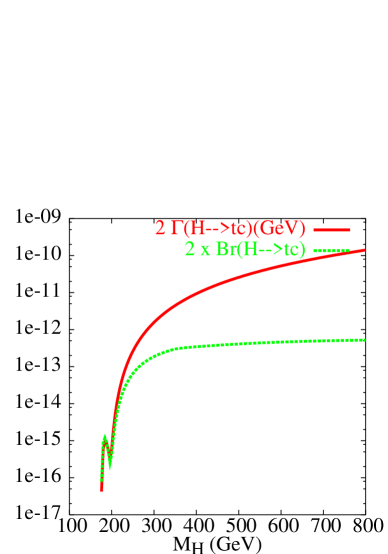
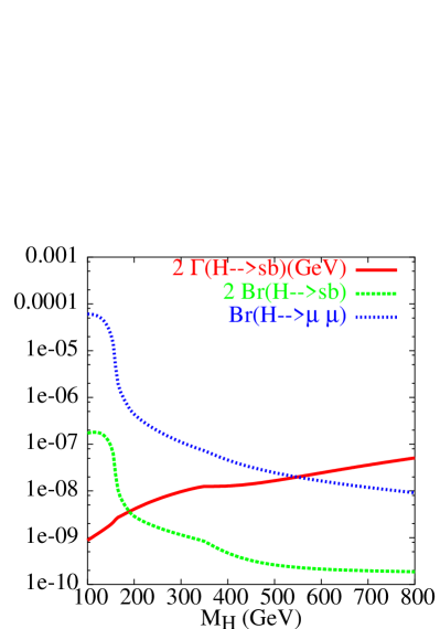
Figure 2: SM width and Branching ratio for $H\to\bar{t}c$ (left) and $H\to\bar{s}b$ (right) as a function of Higgs mass.

In the SM, as expected, the branching ratio of $H\to\bar{t}c$ and $H\to\bar{s}b$ are very suppressed due to GIM mechanism. The branching ratio is very small in both cases for higher Higgs mass $M_{H}\geq 2M_{Z}$ where $H\to W^{+}W^{-}$ and $H\to Z^{0}Z^{0}$ are open.

Both in SM and 2HDM, the decay widths $\Gamma_{\Phi}^{\rm{SM}}$ and $\Gamma_{\Phi}^{\rm{2HDM}}$ of scalar particles: $\Phi=H^{\rm{SM}}$, $h^{0}$, $H^{0}$, $A^{0}$ and $H^{\pm}$ are computed at tree level as follows:

$$\Gamma_{\Phi}^{\rm{SM}}=\sum_{f}\Gamma(\Phi\to f\bar{f})+\Gamma(\Phi\to VV)$$

$$\Gamma_{\Phi}^{\rm{2HDM}}=\sum_{f}\Gamma(\Phi\to f\bar{f})+\Gamma(\Phi\to VV)+\Gamma(\Phi\to VH_{i})+\Gamma(\Phi\to H_{i}H_{j})$$ (16)

QCD corrections to $\Phi\to f\bar{f}$ and $\Phi\to\{gg,\gamma\gamma,\gamma Z,V^{*}V^{*},VV^{*},V^{*}H_{i}\}$ decays are not included in the widths. The decay widths of the Higgs bosons are taken from [31].

For a Higgs mass heavier than 250 GeV, we get branching ratio of the order $10^{-14}\to 10^{-12}$ (resp $10^{-10}\to 10^{-9}$) for $H\to{\bar{t}}c$ (resp $H\to{\bar{s}}b$).
In the case of $H\to{\bar{s}}b$, the branching ratio is enhanced for Higgs boson mass of the order $M_{H}\approx 100\to 120$ GeV where the width of the Higgs is very narrow. We have plotted in Fig. (2) both the decay width and the branching ratios of $H\to{\bar{t}}c$ (left plot) and $H\to{\bar{s}}b$ (right plot) as well as the branching ratio of $H\to\mu^{+}\mu^{-}$. As it can be seen from the right plot $Br(H\to\bar{s}b)$ is two orders of magnitude smaller than $Br(H\to\mu^{+}\mu^{-})$.
Since the decay width of $H\to{\bar{t}}c$ is very suppressed, the threshold for $t\bar{t}$ production is absent in Fig. 2 (left). The situation is slightly different for $H\to\bar{s}b$ where the decay width of $H\to\bar{s}b$ is about 6 order of magnitude larger than decay width of $H\to\bar{t}c$. From the right plot of Fig. (2) one can see that the Br of $H\to\bar{s}b$ is smaller once the $t\bar{t}$ threshold has been passed.

3.2 $h^{0}\to{\bar{s}}b$

Turning now to the 2HDM Higgs bosons FCNC couplings $\Phi\to{\bar{s}}b$, $\Phi=h^{0},H^{0},A^{0}$. The Feynman diagrams are depicted in Fig. (1). The amplitude is sensitive to the $\Phi H^{+}H^{-}$ and $\Phi H^{\pm}G^{\mp}$ couplings through diagrams $d_{12,13,14}$ as well as to the $\Phi t\bar{t}$ and $(H^{-}\bar{b}t)_{L,R}$ couplings through diagrams $d_{11,12,13,14}$. In 2HDM, it is expected that the dominant contribution to the amplitude of $\Phi^{0}\to\bar{s}b$ comes from diagram $d_{12}$. The amplitude of $d_{12}$ is proportional to the trilinear Higgs coupling $\Phi^{0}H^{+}H^{-}$ and is given by ($\Phi=h^{0},H^{0}$):

$$M_{d_{12}}=\Phi^{0}H^{+}H^{-}\frac{\alpha V_{ts}}{8\pi}\frac{M_{t}^{2}}{\tan^{2}\beta}\frac{M_{b}}{8M_{W}^{2}s_{W}^{2}}[(1+\tan\beta Y_{b})C_{0}+C_{1}+C_{2}]\bar{v}(M_{s})\frac{1+\gamma_{5}}{2}u(M_{b})$$ (17)

where we have neglected the strange quark mass. In the conventions of [29], the arguments of the Passarino-Veltman functions $C_{i}$ are $\{M_{b}^{2},M_{s}^{2},M_{\Phi}^{2},M_{H\pm}^{2},M_{t}^{2},M_{H\pm}^{2}\}$. The Yukawa coupling $Y_{b}$ of the bottom is model dependant and is given by $Y_{b}=-1/\tan\beta$ (resp $Y_{b}=\tan\beta$) for 2HDM-I (resp 2HDM-II).
In 2HDM-I, $1+\tan\beta Y_{b}=0$, the amplitude of $d_{12}$ is enhanced by $\frac{M_{t}^{2}}{\tan^{2}\beta}$ factor for small $\tan\beta$ as well as by the trilinear coupling $\Phi^{0}H^{+}H^{-}$.

The diagram $d_{11}$ is sensitive to the coupling $\Phi^{0}\bar{t}t$. It is clear from equation (9) that the top effect is enhanced for small $\tan\beta$ in the case of CP-odd $A^{0}$ boson. While in the case of CP-even $H^{0}$ and $h^{0}$, the couplings are enhanced at small $\tan\beta$ and large $\sin\alpha$ (resp large $\cos\alpha$) for $H^{0}$ (resp $h^{0}$). Consequently, our numerics are presented for small $\tan\beta=0.3$, $\sin\alpha=0.1$ for $h^{0}\to{\bar{s}}b$ and $\sin\alpha=0.95$ for $H^{0}\to{\bar{s}}b$.
We also give other numerical results for specific 2HDM parameters where $Br(h^{0}\to\bar{s}b)$ and $Br(H^{0}\to\bar{s}b)$ get their maximum values without violating $\delta\rho$ and perturbativity constraints.

    

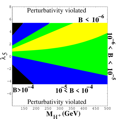
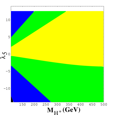
Figure 3: Contours for $2\times Br(h^{0}\to\bar{s}b)$ in 2HDM-II $\tan\beta=0.3$ (left), $\tan\beta=1.5$ (right) in the ($M_{H\pm}$, $\lambda_{5}$) plane with $M_{h}=110$ GeV, $M_{H}=180$ GeV, $\sin\alpha=0.1$ and $M_{A^{0}}=M_{H\pm}$

We show in Fig. (3) contour plots for $Br(h^{0}\to\bar{s}b)$ in 2HDM-II $\tan\beta=0.3$ (left) and $\tan\beta=1.5$ GeV (right) in the ($M_{H\pm}$, $\lambda_{5}$) plane. $\lambda_{5}$ is varied in the perturbative range $|\lambda_{5}|<4\pi$. The other inputs are $M_{h}=110$ GeV, $M_{H}=180$ GeV, $\sin\alpha=0.1$ and $M_{A^{0}}=M_{H\pm}$. The width $\Gamma_{h^{0}}$ is computed at tree level according to eq. (16). Since the mass of $h^{0}$ is taken at 110 GeV, only light fermions contribute to $\Gamma_{h^{0}}$ and so the width is very narrow and is of the order $57\times 10^{-4}$ (resp $83\times 10^{-5}$ GeV) at $\tan\beta=0.3$ (resp $\tan\beta=1.5$). Such narrow width could enhance the branching ratio $Br(h^{0}\to\bar{s}b)$. We would like to mention first that for this set of parameters, the perturbativity of scalar quartic couplings $\lambda_{i}$ is violated around $\lambda_{5}\mathrel{\raise 1.29167pt\hbox{$>$\kern-7.5pt\lower 4.30554pt\hbox{$\sim$}}}5.5$. We get $|\lambda_{1}|>4\pi$ for $\tan\beta=0.3$, while for $\tan\beta=1.5$ there is no such bound.

Large branching ratios can be obtained for light charged Higgs mass. This can be seen in the left panel black and blue areas of Fig. (3) which correspond to small $\tan\beta=0.3$ and large $|\lambda_{5}|$. In those areas the coupling $h^{0}H^{+}H^{-}$ gets its largest value (see also Fig. (4)). In this case one can obtain branching ratio in the range: $10^{-4}<Br(h^{0}\to\bar{s}b)<6\times 10^{-4}$ for $M_{H\pm}<200$ GeV , $\lambda_{5}\mathrel{\raise 1.29167pt\hbox{$<$\kern-7.5pt\lower 4.30554pt\hbox{$\sim$}}}-1.2$ and $\lambda_{5}\mathrel{\raise 1.29167pt\hbox{$>$\kern-7.5pt\lower 4.30554pt\hbox{$\sim$}}}3$. For charged Higgs mass greater than 200 GeV, there is also a region where the branching ratio can be in the range $10^{-5}\to 10^{-4}$. This can be achieved by taking large and negative $\lambda_{5}\mathrel{\raise 1.29167pt\hbox{$<$\kern-7.5pt\lower 4.30554pt\hbox{$\sim$}}}-1$. In the case of positive $\lambda_{5}$ and $M_{H\pm}\mathrel{\raise 1.29167pt\hbox{$>$\kern-7.5pt\lower 4.30554pt\hbox{$\sim$}}}250$ GeV, the branching ratio decreases to a value $\mathrel{\raise 1.29167pt\hbox{$<$\kern-7.5pt\lower 4.30554pt\hbox{$\sim$}}}10^{-5}$.

When $\tan\beta=1.5$, the coupling $h^{0}t\bar{t}$ is reduced, and we are left only with a small region where the branching ratio $Br(h^{0}\to\bar{s}b)$ is of the order $10^{-5}\to 10^{-4}$ for $M_{H\pm}\mathrel{\raise 1.29167pt\hbox{$<$\kern-7.5pt\lower 4.30554pt\hbox{$\sim$}}}250$ GeV and large $|\lambda_{5}|\mathrel{\raise 1.29167pt\hbox{$>$\kern-7.5pt\lower 4.30554pt\hbox{$\sim$}}}5$. In both plots (left and right), the coupling $h^{0}H^{+}H^{-}$ reaches its minimal value in the region where $\lambda_{5}\approx 0\to 2$, which explains why the branching ratio is so small in this region.

Now we turn to the case where $M_{H\pm}\neq M_{A}$, $\delta\rho\neq 0$. We have performed a systematic scan over the full 2HDM parameters space taking into account $\delta\rho$ and perturbativity constraints. The maximum branching ratios found for $h^{0}\to\bar{s}b$ in 2HDM-I and II are displayed in table 1. We show not only width and Br of $h^{0}\to\bar{s}b$ but also the width and Br of $h^{0}\to\gamma\gamma$ for comparison. The total width of the Higgs $\Gamma_{h^{0}}$ is also given. When $\Gamma_{h^{0}}$ becomes comparable to the width of $h^{0}\to\bar{s}b$ and/or $h^{0}\to\gamma\gamma$, those decays widths have to be included in the total width $\Gamma_{h^{0}}$ in order to compute the Br${}_{\bar{s}b}$ and Br_γγ.

$\begin{array}[]{c}M_{h}\\ M_{H}\end{array}\begin{array}[]{c}M_{H\pm}\\ M_{A}\end{array}$	$\begin{array}[]{c}\sin\alpha\\ \tan\beta\end{array}$	$\lambda_{5}$	$2\times$ Br${}_{\bar{s}b}$	$2\times$ $\Gamma_{\bar{s}b}$	$2\times$ Brγγ	$2\times\Gamma_{\gamma\gamma}$	$\Gamma_{h}$
$\begin{array}[]{c}95\\ 340\end{array}\begin{array}[]{c}100\\ 110\end{array}$	$\begin{array}[]{c}-.98\\ .2\end{array}$	6	$\begin{array}[]{c}10^{-3}\\ 7\times 10^{-4}\end{array}$	$\begin{array}[]{c}6\times 10^{-6}\\ 3\times 10^{-6}\end{array}$	$\begin{array}[]{c}6\times 10^{-3}\\ 6\times 10^{-3}\end{array}$	$\begin{array}[]{c}3\times 10^{-5}\\ 3\times 10^{-5}\end{array}$	$\begin{array}[]{c}5\times 10^{-3}\\ 5\times 10^{-3}\end{array}$
$\begin{array}[]{c}140\\ 340\end{array}\begin{array}[]{c}110\\ 100\end{array}$	$\begin{array}[]{c}-.96\\ .25\end{array}$	6	$\begin{array}[]{c}4\times 10^{-4}\\ 3\times 10^{-4}\end{array}$	$\begin{array}[]{c}4\times 10^{-6}\\ 2\times 10^{-6}\end{array}$	$\begin{array}[]{c}10^{-2}\\ 2\times 10^{-2}\end{array}$	$\begin{array}[]{c}10^{-4}\\ 10^{-4}\end{array}$	$\begin{array}[]{c}9\times 10^{-3}\\ 7\times 10^{-3}\end{array}$
$\begin{array}[]{c}135\\ 160\end{array}\begin{array}[]{c}105\\ 240\end{array}$	$\begin{array}[]{c}-.98\\ .46\end{array}$	-12	$\begin{array}[]{c}10^{-3}\\ 2\times 10^{-4}\end{array}$	$\begin{array}[]{c}2\times 10^{-6}\\ 10^{-6}\end{array}$	$\begin{array}[]{c}7\times 10^{-3}\\ 2\times 10^{-3}\end{array}$	$\begin{array}[]{c}10^{-5}\\ 10^{-5}\end{array}$	$\begin{array}[]{c}2\times 10^{-3}\\ 7\times 10^{-3}\end{array}$
$\begin{array}[]{c}115\\ 250\end{array}\begin{array}[]{c}110\\ 190\end{array}$	$\begin{array}[]{c}.1\\ .1\end{array}$	0	$\begin{array}[]{c}9\times 10^{-4}\\ 10^{-3}\end{array}$	$\begin{array}[]{c}5\times 10^{-4}\\ 5\times 10^{-5}\end{array}$	$\begin{array}[]{c}2\times 10^{-4}\\ 3\times 10^{-3}\end{array}$	$\begin{array}[]{c}10^{-4}\\ 10^{-4}\end{array}$	$\begin{array}[]{c}.55\\ 5\times 10^{-2}\end{array}$
$\begin{array}[]{c}110\\ 210\end{array}\begin{array}[]{c}105\\ 150\end{array}$	$\begin{array}[]{c}.18\\ .1\end{array}$	0	$\begin{array}[]{c}9\times 10^{-4}\\ 10^{-3}\end{array}$	$\begin{array}[]{c}5\times 10^{-4}\\ 5\times 10^{-5}\end{array}$	$\begin{array}[]{c}2\times 10^{-4}\\ 3\times 10^{-3}\end{array}$	$\begin{array}[]{c}10^{-4}\\ 10^{-4}\end{array}$	$\begin{array}[]{c}.52\\ 5\times 10^{-2}\end{array}$

Table 1: Maximum Branching ratios of $h^{0}\to\bar{s}b$ in 2HDM-I and II and corresponding 2HDM parameters, all masses and decay width are in GeV. In $Br$ and widths $\Gamma$ columns, the upper row is for 2HDM-I and the down row is for 2HDM-II

The first three columns of table 1 are for 2HDM parameters. From 4th to 8th columns we give Br and widths. In those columns, the upper row is for 2HDM-I and the down row is for 2HDM-II.
In 2HDM-I, Br$(h^{0}\to\bar{s}b)$ of the order $10^{-3}$ can be reached in the limit $\sin\alpha\to-0.98$ ($\alpha\to-\pi/2$) and small $\tan\beta\leq 0.5$. In fact, this limit ($\alpha\to-\pi/2$) is very close to fermiophobic scenario $\alpha=\pm\pi/2$. In the fermiophobic limit, all couplings of $h^{0}$ to down quarks and leptons are suppressed eq. (10). In this limit, $h^{0}\bar{t}t$ is also suppressed eq. (9). The width of light Higgs $h^{0}$ ($M_{h}<160$ GeV) is then very tiny in the limit $\sin\alpha\to-0.98$. This tiny width together with large $h^{0}H^{+}H^{-}$ are the sources of enhancement of the Br$(h^{0}\to\bar{s}b)$ to $10^{-3}$ level. This can be seen in the first, second and third lines of table 1
In 2HDM-II, the couplings of $h^{0}$ to down quarks and leptons are suppressed for $\sin\alpha\approx 0.1$ eq. (11). Hence, the width of light Higgs ($M_{h}<160$ GeV) is very tiny in the limit $\sin\alpha\approx 0.1$. Moreover, in this limit, the coupling $h^{0}\bar{t}t$ is enhanced in both models 2HDM-I and II. The decay width $\Gamma(h^{0}\to{\bar{s}b})$ which was $\approx 10^{-6}$ for $\sin\alpha=-0.98$ is of the order $\approx 10^{-5}$ for $\sin\alpha=0.1$. Consequently, the Br$(h^{0}\to\bar{s}b)$ reaches $10^{-3}$.
In this scenario, as one can see from table 1, the Br$(h^{0}\to\gamma\gamma)$ in 2HDM-I is $2\times 10^{-4}$ which is smaller than Br$(h^{0}\to\bar{s}b)=9\times 10^{-4}$. This is mainly due to the fact that the trilinear coupling $h^{0}H^{+}H^{-}$ is very suppressed in this scenario (see more details in next section).
As one can see from the last line of the table 1, there exist also values of $\sin\alpha=0.18$, far from fermiophobic scenario but with small $\lambda_{5}=0$, where Br$(h^{0}\to\bar{s}b)$ can be of the order $10^{-3}$.

    

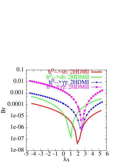
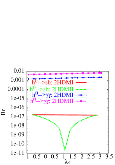
Figure 4: $2\times Br(h^{0}\to\gamma\gamma)$ and $2\times Br(h^{0}\to\bar{s}b)$ in 2HDM-I and II, $m_{H\pm}=100$ GeV, $\tan\beta=0.3$ (left) and $\tan\beta=5$ (right). All the other parameters are the same as in Fig. (3).

3.3 Can $h^{0}\to\bar{s}b$ compete with $h^{0}\to\gamma\gamma$?

It is well known that the decay $h^{0}\to\gamma\gamma$ is loop induced and so is suppressed. In the SM, the branching ratio $Br(H^{SM}\to\gamma\gamma)$ is about $\approx 10^{-3}$ for Higgs mass in the range $M_{H}=100\to 160$ GeV. Hence, with maximum branching ratio for $h^{0}\to\bar{s}b$ of the order $1\times 10^{-4}\to 6\times 10^{-4}$ in 2HDM-I or II, it is legitimate to compare $h^{0}\to\gamma\gamma$ and $h^{0}\to\bar{s}b$ in 2HDM-I or II. Of course, even if $h^{0}\to\bar{s}b$ and $h^{0}\to\gamma\gamma$ has a competitive branching ratio, we should keep in mind that $h^{0}\to\gamma\gamma$ decay has a clear signature while the FCNC decay $h^{0}\to\bar{s}b$ has not.

We illustrate in Fig. (4) the branching ratio for $h^{0}\to\bar{s}b$ and $h^{0}\to\gamma\gamma$ both in 2HDM-I and II. The charged Higgs mass is fixed to 100 GeV. It is clear that in the case $\tan\beta=0.3$ $h^{0}\to\gamma\gamma$ is about one order of magnitude bigger than $h^{0}\to\bar{s}b$. While, in the case of $\tan\beta=5$ $h^{0}\to\gamma\gamma$ is more than four orders of magnitude bigger than $h^{0}\to\bar{s}b$. This is because at $\tan\beta=0.3$ (resp $\tan\beta=5$) the W loop are suppressed by a factor $h^{0}W^{+}W^{-}\propto\sin(\beta-\alpha)\approx 0.2$ (resp enhanced by $h^{0}W^{+}W^{-}\propto\sin(\beta-\alpha)\approx 0.96$). All the dips observed in the plots correspond to the minimum of the coupling $h^{0}H^{-}H^{+}$. Those dips are not located at the same $\lambda_{5}$, this is due to a destructive interference with others diagrams. When $h^{0}H^{-}H^{+}$ coupling is very suppressed, it may be possible that the Br$(h^{0}\to\bar{s}b)$ could be higher than Br$(h^{0}\to\gamma\gamma)$ as it can be seen both in the left plot of Fig. (4) for $\lambda_{5}=2.5$ and in table 1 for $\sin\alpha=0.1$ in 2HDM-II.
However, even if Br$(h^{0}\to\gamma\gamma)$ and Br$(h^{0}\to\bar{s}b)$ become comparable, we should keep in mind that $h^{0}\to\gamma\gamma$ has a very clear signature while $h^{0}\to\bar{s}b$ does not.

An interesting feature of the 2HDM-I, is its fermiophobic scenario. The light CP-even Higgs $h^{0}$ of the 2HDM-I is fermiophobic in the limit $\alpha\to\pi/2$, all $h^{0}$ couplings to fermions vanishes for $\alpha=\pi/2$ [32, 18]. If $h^{0}$, with a mass in the range $100\to 160$ GeV, is fermiophobic the dominant decay mode is $h^{0}\to\gamma\gamma$. It has been shown in Ref. [33] that in the fermiophobic limit, the branching ratio of the one loop induced decay $h^{0}\to\bar{b}b$ is below $10\%\to 30\%$. As the decay $h^{0}\to\bar{s}b$ is concerned, we have checked by systematic scan that in the fermiophobic limit, the decay width of $h^{0}\to\gamma\gamma$ is more than one order of magnitude bigger than the width of $h^{0}\to\bar{s}b$.

3.4 $H^{0}\to{\bar{s}}b$

    

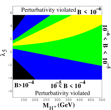
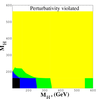
Figure 5: Contours for $2\times Br(H^{0}\to\bar{s}b)$ in 2HDM-II in the plan ($M_{H\pm}$, $\lambda_{5}$) $M_{H}=140$ GeV (left), ($M_{H\pm}$, $M_{H}$) $\lambda_{5}=5$ (right) with $\tan\beta=0.3$, $M_{h}=110$ GeV, $\sin\alpha=0.95$ and $M_{A^{0}}=M_{H\pm}$

We now discuss the heavy CP-even decay $H^{0}\to\bar{s}b$. Our numerical results are shown in Fig. (5). To maximize the coupling $H^{0}\bar{t}t$, we choose of course small $\tan\beta\approx 0.3$ and large $\sin\alpha\approx 0.95$. In the right plot of Fig. (5), we show contour plots for $Br(H^{0}\to\bar{s}b)$ in the plane $(M_{H\pm},\lambda_{5})$ for $M_{H}=140$ GeV. For CP-even Higgs mass 140 GeV, $H^{0}\to W^{+}W^{-}$, $H^{0}\to ZZ$, $H^{0}\to\bar{t}t$, $H^{0}\to A^{0}Z$ and $H^{0}\to H_{i}H_{j}$ are not yet open, and so the width is narrow. In particular, for the set of parameters fixed here: $M_{h}=110$ GeV, $\sin\alpha=0.95$ and $M_{A^{0}}=M_{H\pm}$, the width is $73\times 10^{-4}$ GeV.
The behavior is similar to what we obtain for $Br(h^{0}\to\bar{s}b)$. In the black regions (large $\lambda_{5}$), the coupling $H^{0}H^{+}H^{-}$ is maximal while for $\lambda_{5}\in[0,2]$ $H^{0}H^{+}H^{-}$ is minimal. In the black region the branching ratio of $Br(H^{0}\to\bar{s}b)$ can reach $\approx 7\times 10^{-4}$. From the left panel of Fig. (5), it is evident that there is a relatively large region in the plane ($M_{H\pm},\lambda_{5}$) where the $Br(H^{0}\to\bar{s}b)\mathrel{\raise 1.29167pt\hbox{$>$\kern-7.5pt\lower 4.30554pt\hbox{$\sim$}}}10^{-5}$.

$\begin{array}[]{c}M_{h}\\ M_{H}\end{array}\begin{array}[]{c}M_{H\pm}\\ M_{A}\end{array}$	$\begin{array}[]{c}\sin\alpha\\ \tan\beta\end{array}$	$\lambda_{5}$	$2\times$ Br${}_{\bar{s}b}$	$2\times$ $\Gamma_{\bar{s}b}$	$2\times$ Brγγ	$2\times\Gamma_{\gamma\gamma}$	$\Gamma_{H}$
$\begin{array}[]{c}115\\ 155\end{array}\begin{array}[]{c}142\\ 183\end{array}$	$\begin{array}[]{c}.1\\ .5\end{array}$	-12	$\begin{array}[]{c}10^{-3}\\ 4\times 10^{-5}\end{array}$	$\begin{array}[]{c}5\times 10^{-7}\\ 4\times 10^{-7}\end{array}$	$\begin{array}[]{c}3\times 10^{-2}\\ 10^{-3}\end{array}$	$\begin{array}[]{c}10^{-5}\\ 10^{-5}\end{array}$	$\begin{array}[]{c}4\times 10^{-4}\\ 8\times 10^{-3}\end{array}$
$\begin{array}[]{c}100\\ 155\end{array}\begin{array}[]{c}115\\ 103\end{array}$	$\begin{array}[]{c}.1\\ .34\end{array}$	-6	$\begin{array}[]{c}2\times 10^{-3}\\ 8\times 10^{-5}\end{array}$	$\begin{array}[]{c}10^{-6}\\ 6\times 10^{-7}\end{array}$	$\begin{array}[]{c}2\times 10^{-2}\\ 2\times 10^{-3}\end{array}$	$\begin{array}[]{c}2\times 10^{-5}\\ 2\times 10^{-5}\end{array}$	$\begin{array}[]{c}7\times 10^{-4}\\ 8\times 10^{-3}\end{array}$
$\begin{array}[]{c}100\\ 155\end{array}\begin{array}[]{c}120\\ 140\end{array}$	$\begin{array}[]{c}.08\\ .45\end{array}$	12	$\begin{array}[]{c}2\times 10^{-3}\\ 8\times 10^{-5}\end{array}$	$\begin{array}[]{c}7\times 10^{-7}\\ 6\times 10^{-7}\end{array}$	$\begin{array}[]{c}.73\\ 3\times 10^{-2}\end{array}$	$\begin{array}[]{c}2\times 10^{-4}\\ 2\times 10^{-4}\end{array}$	$\begin{array}[]{c}3\times 10^{-4}\\ 8\times 10^{-3}\end{array}$
$\begin{array}[]{c}100\\ 125\end{array}\begin{array}[]{c}115\\ 103\end{array}$	$\begin{array}[]{c}-.98\\ .1\end{array}$	0	$\begin{array}[]{c}9\times 10^{-4}\\ 10^{-3}\end{array}$	$\begin{array}[]{c}5\times 10^{-4}\\ 6\times 10^{-5}\end{array}$	$\begin{array}[]{c}3\times 10^{-4}\\ 4\times 10^{-3}\end{array}$	$\begin{array}[]{c}2\times 10^{-4}\\ 2\times 10^{-4}\end{array}$	$\begin{array}[]{c}.58\\ 5\times 10^{-2}\end{array}$
$\begin{array}[]{c}100\\ 130\end{array}\begin{array}[]{c}110\\ 300\end{array}$	$\begin{array}[]{c}.9\\ .1\end{array}$	0	$\begin{array}[]{c}10^{-3}\\ 10^{-3}\end{array}$	$\begin{array}[]{c}5\times 10^{-4}\\ 6\times 10^{-5}\end{array}$	$\begin{array}[]{c}2\times 10^{-4}\\ 2\times 10^{-3}\end{array}$	$\begin{array}[]{c}10^{-4}\\ 10^{-4}\end{array}$	$\begin{array}[]{c}.51\\ 5\times 10^{-2}\end{array}$
$\begin{array}[]{c}100\\ 145\end{array}\begin{array}[]{c}115\\ 103\end{array}$	$\begin{array}[]{c}-.58\\ .1\end{array}$	0	$\begin{array}[]{c}9\times 10^{-4}\\ 10^{-3}\end{array}$	$\begin{array}[]{c}2\times 10^{-4}\\ 3\times 10^{-5}\end{array}$	$\begin{array}[]{c}10^{-3}\\ 10^{-2}\end{array}$	$\begin{array}[]{c}2\times 10^{-4}\\ 3\times 10^{-4}\end{array}$	$\begin{array}[]{c}.24\\ 3\times 10^{-2}\end{array}$

Table 2: Maximum Branching ratios of $H^{0}\to\bar{s}b$ in 2HDM-I and II and corresponding 2HDM parameters, all masses and decay width are in GeV. In $Br$ and widths $\Gamma$ columns, the upper row is for 2HDM-I and the down row is for 2HDM-II

In the right panel of Fig. (5), we show $Br(H^{0}\to\bar{s}b)$ in the plan $(M_{H},M_{H\pm})$ for $\lambda_{5}=5$. One can see that when CP-even mass $M_{H}<2M_{W}$, the decay $H^{0}\to W^{+}W^{-}$ is not yet open. The width $\Gamma_{H^{0}}$ is narrow, and so the branching ratio is large. For $M_{H\pm}<250$ GeV and $M_{H}<2M_{W}$, one can have $Br(H^{0}\to\bar{s}{b})\mathrel{\raise 1.29167pt\hbox{$>$\kern-7.5pt\lower 4.30554pt\hbox{$\sim$}}}10^{-5}$. Once the CP-even Higgs mass $M_{H}>2M_{W}$, the decay $H^{0}\to W^{+}W^{-}$ is open, and the width is larger than $5\times 10^{-2}$ GeV. The Branching ratio $Br(H^{0}\to\bar{s}{b})$ is then reduced. As it can be seen from the right plot, for $M_{H}\mathrel{\raise 1.29167pt\hbox{$>$\kern-7.5pt\lower 4.30554pt\hbox{$\sim$}}}220$ GeV, the branching ratio $Br(H^{0}\to\bar{s}{b})$ is less than $\mathrel{\raise 1.29167pt\hbox{$<$\kern-7.5pt\lower 4.30554pt\hbox{$\sim$}}}10^{-6}$.

In case of 2HDM-I, both $h^{0}t\bar{t}$, $H^{0}\bar{t}t$ and $(H^{-}\bar{b}t)_{R}$ couplings are the same as in 2HDM-II, while $(H^{-}\bar{b}t)_{L}$ which is proportional to $M_{b}\tan\beta$ in 2HDM-II is now proportional to $M_{b}/\tan\beta$. For small $\tan\beta\approx 0.3$, both $Br(h^{0}\to\bar{s}b)$ and $Br(H^{0}\to\bar{s}b)$ are of the same order as in 2HDM-II, while for large $\tan\beta$ those Branching ratios are less than about $\approx 10^{-6}$.

In case where $M_{H\pm}\neq M_{A}$ ($\delta\rho\neq 0$), we present our results of maximum branching ratios of $H^{0}\to\bar{s}b$ in the table 2. It turns out that in 2HDM-I (resp 2HDM-II), Br$(H^{0}\to\bar{s}b)$ reach $10^{-3}$ for small $\sin\alpha\approx 0.1$ (resp large $|\sin\alpha|\approx 0.9$). The interpretation is the same as in the case of light CP even Higgs $h^{0}$. In 2HDM-I (resp 2HDM-II), the couplings of $H^{0}$ to down quarks and leptons are suppressed for $\sin\alpha\approx 0.1$ (resp $|\sin\alpha|\approx 0.9$). In those cases the total Higgs width is very tiny and so the branching ratio of $H^{0}\to\bar{s}b$ is enhanced.
Of course, Br$(H^{0}\to\bar{s}b)$ reach $10^{-3}$ only for light charged Higgs, which is strongly disfavored by $b\to s\gamma$ constraint [24] in 2HDM-II.
From table 2, one can see also that in 2HDM-II and for $\sin\alpha\approx\{0.9,-0.98\}$ the Br$(H^{0}\to\bar{s}b)$ and Br$(H^{0}\to\gamma\gamma)$ are of comparable size. This is again mainly due to the suppression of the coupling $H^{0}H^{+}H^{-}$ in those limits.
As in the case of light CP-even Higgs $h^{0}$, there exist values of $\sin\alpha=-0.58$ far from fermiophobic limit with small $\lambda_{5}=0$ where Br$(H^{0}\to\bar{s}b)$ can reach $10^{-3}$.

3.5 $A^{0}\to{\bar{s}}b$

Let us now look at 2HDM contribution to $A^{0}\to\bar{s}b$. Since $A^{0}$ is CP-odd, it does not couple to a pair of charged Higgs. The only pure trilinear scalar coupling which contributes to $A^{0}\to\bar{s}b$ is $A^{0}H^{\pm}G^{\mp}$ eq. (8). Unlike the couplings $H^{0}H^{+}H^{-}$ and $h^{0}H^{+}H^{-}$ eqs (4,6), which depend both on Higgs masses, $\tan\beta$ as well as the soft breaking term $\lambda_{5}$, the coupling $A^{0}H^{\pm}G^{\mp}$ depends only on the splitting $M_{H\pm}^{2}-M_{A}^{2}$. As mentioned above, such splitting should not be too large, otherwise the $\delta\rho$ constraint is not satisfied. As one can read from eqs. (9,13), the couplings $A^{0}\bar{t}t$ and $(H^{-}\bar{b}t)_{R}$ are proportional to $M_{t}/\tan\beta$. Hence enhancement is expected at small $\tan\beta$.

    

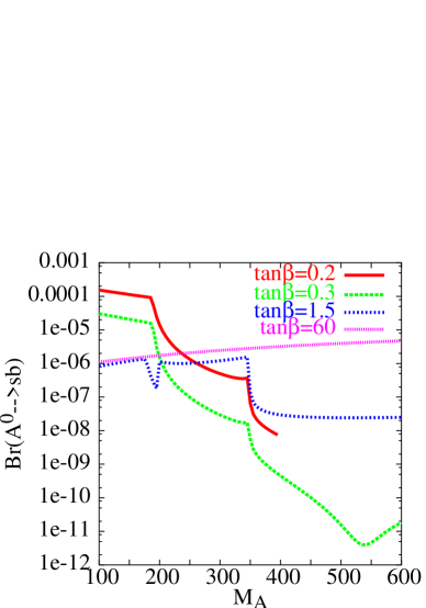
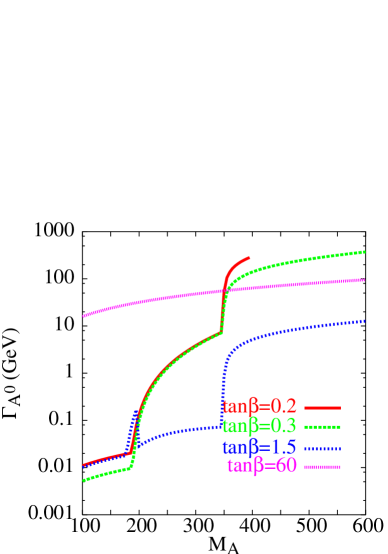
Figure 6: $2\times Br(A^{0}\to\bar{s}b)$ (left) and CP-odd $A^{0}$ width $\Gamma_{A^{0}}$ (right) as function of $M_{A}$ for several values of $\tan\beta$

As we stressed before, our 2HDM parameters in this case are: $\tan\beta$, $M_{A}$ and $M_{H\pm}$. For simplification, we use the MSSM sum-rules to fix charged Higgs mass and $\alpha$ by using $\tan\beta$, CP-odd mass $M_{A}$ and a SUSY scale which we take at 1 TeV. CP-odd mass will be varied from 100 GeV to 600 GeV without worrying about perturbativity. $\tan\beta$ is taken to be $\mathrel{\raise 1.29167pt\hbox{$>$\kern-7.5pt\lower 4.30554pt\hbox{$\sim$}}}0.1$.
We present our numerical results for $A^{0}\to\bar{s}b$ in 2HDM-II in Fig. (6). As can be seen from the left plot, the Branching ratio $Br(A^{0}\to\bar{s}b)$ is greater than $10^{-5}$ only for small $\tan\beta\approx 0.1\to 0.35$ and light $M_{A}$ and $M_{H\pm}$. For light $M_{A}\mathrel{\raise 1.29167pt\hbox{$<$\kern-7.5pt\lower 4.30554pt\hbox{$\sim$}}}200$ GeV and low $\tan\beta\mathrel{\raise 1.29167pt\hbox{$<$\kern-7.5pt\lower 4.30554pt\hbox{$\sim$}}}1$, the width of $A^{0}$ is still small and so the branching ratio is enhanced. For $M_{A}\mathrel{\raise 1.29167pt\hbox{$>$\kern-7.5pt\lower 4.30554pt\hbox{$\sim$}}}200$ GeV, the decay $A^{0}\to h^{0}Z$ is open and the decay width $\Gamma_{A^{0}}$ increases. Therefore, the branching ratio is reduced. Note that for $\tan\beta=0.2$, we cut off the curve at $M_{A}\approx 400$ GeV where the width $\Gamma_{A^{0}}$ starts to be greater than $M_{A}$. At large $\tan\beta$, due to the bottom Yukawa coupling, both the partial width $\Gamma(A^{0}\to\bar{s}b)$ and total width $\Gamma_{A^{0}}$ are enhanced, and the branching ratio is saturated in the range $[10^{-6},10^{-5}]$.
The situation is almost the same in 2HDM-I.

4 Conclusions

In the framework of the 2HDM with natural flavor conservation, we have studied various Higgs FCNC $\Phi\to\bar{s}b$. The study has been carried out taking into account the experimental constraint on the $\rho$ parameter and also perturbativity constraints on all the scalar quartic couplings $\lambda_{i}$. Numerical results for the branching ratios have been discussed. We emphasized the effect coming from both top and bottom Yukawa couplings and pure trilinear scalar couplings such as $h^{0}H^{+}H^{-}$ and $H^{0}H^{+}H^{-}$.
We have shown that, in 2HDM-I and 2HDM-II, the branching ratios of Higgs FCNC $\{h^{0},H^{0},A^{0}\}\to\bar{s}b$ are enhanced to the range of $10^{-4}\to 7\times 10^{-4}$ for small $\tan\beta$, rather light charged Higgs boson and large soft breaking term $\lambda_{5}$. The branching ratio of $Br(\{h^{0},H^{0}\}\to\bar{s}b)$ can be pushed to $10^{-3}$ level when $\sin\alpha$ is close to fermiophobic limit ($\sin\alpha\approx-0.98$) or $\sin\alpha\approx 0.1$ and even for $\sin\alpha$ far from those limits but with small $\lambda_{5}=0$.
Charged Higgs mass of 2HDM-I is not constrained by $b\to s\gamma$, $Br(\{h^{0},H^{0}\}\to\bar{s}b)$ can be of the order $10^{-4}\to 10^{-3}$ for light charged Higgs which is comparable to size of SUSY predictions [12, 14]. Those branching ratios rates, could still leads to large number of events at LHC [11].
In 2HDM-II with $b\to s\gamma$ constraint, branching ratios of $\{h^{0},H^{0}\}\to\bar{s}b$ are smaller than $10^{-5}$ (resp $10^{-4}$) for $\tan\beta>1$ (resp $\tan\beta<1$).
In the case of light CP-even $m_{h^{0}}\approx 100\to 160$ GeV, we have also shown that the branching ratio of $Br(h^{0}\to\bar{s}b)$ is well below $Br(h^{0}\to\gamma\gamma)$ in most of the case. This is also the case in the fermiophobic scenario of 2HDM-I.
One interesting scenario is that both $Br(h^{0}\to\gamma\gamma)$ and $Br(h^{0}\to\bar{s}b)$ develop a dips for some $\lambda_{5}$ (see Fig. 4). Those dips are not located at the same $\lambda_{5}$ due to the presence of diagrams which contribute to $h^{0}\to\bar{s}b$ but not to $h^{0}\to\gamma\gamma$. The dip for $Br(h^{0}\to\bar{s}b)$ is located for $\lambda_{5}=1$ while for $Br(h^{0}\to\gamma\gamma)$ it is located for $\lambda_{5}\approx 2.5$. For $\lambda_{5}\approx 2.5$, we are already away from $Br(h^{0}\to\bar{s}b)$ dip, the $Br(h^{0}\to\bar{s}b)$ is slightly higher than $Br(h^{0}\to\gamma\gamma)$.

Acknowledgments This work was done within the framework of the Associate Scheme of ICTP. Thanks to Thomas Hahn for his help. We also want to thank Andrew Akeroyd for discussions and for reading the manuscript.

References

- [1] M. Beneke, I. Efthymipopulos, M. L. Mangano, J. Womersley (conveners) et al., report in the Workshop on Standard Model Physics (and more) at the LHC, Geneva, hep-ph/0003033
- [2] J. A. Aguilar-Saavedra et al. [ECFA/DESY LC Physics Working Group Collaboration], arXiv:hep-ph/0106315.
- [3] G. Eilam, J. L. Hewett and A. Soni, Phys. Rev. D 44 (1991) 1473 [Erratum-ibid. D 59 (1999) 039901].
- [4] B. Mele, S. Petrarca and A. Soddu, Phys. Lett. B435, 401 (1998)
- [5] J. A. Aguilar-Saavedra, Acta Phys. Polon. B 35 (2004) 2695 [arXiv:hep-ph/0409342]. E. W. N. Glover et al., Acta Phys. Polon. B 35 (2004) 2671 [arXiv:hep-ph/0410110]. 0409342,0410110
- [6] T. P. Cheng and M. Sher, Phys. Rev. D 35, 3484 (1987).
- [7] W. S. Hou, Phys. Lett. B 296, 179 (1992).
- [8] D. Atwood, L. Reina and A. Soni, Phys. Rev. D55, 3156 (1997)
- [9] D. Atwood, L. Reina and A. Soni, Phys. Rev. D 53, 1199 (1996) [arXiv:hep-ph/9506243]. W. S. Hou, G. L. Lin and C. Y. Ma, Phys. Rev. D 56, 7434 (1997).
- [10] S. Béjar, J. Guasch and J. Solà, Nucl. Phys. B 600, 21 (2001) [arXiv:hep-ph/0011091]; [arXiv:hep-ph/0101294].
- [11] S. Béjar, J. Guasch and J. Solà, Nucl. Phys. B 675, 270 (2003).
- [12] A. M. Curiel, M. J. Herrero, W. Hollik, F. Merz and S. Peñaranda, Phys. Rev. D 69, 075009 (2004). A. M. Curiel, M. J. Herrero and D. Temes, Phys. Rev. D 67, 075008 (2003).
- [13] D. A. Demir, Phys. Lett. B 571, 193 (2003).
- [14] S. Béjar, F. Dilme, J. Guasch and J. Solà, JHEP 0408, 018 (2004).
- [15] J. Guasch and J. Solà, Nucl. Phys. B 562, 3 (1999) [arXiv:hep-ph/9906268].
- [16] J. M. Yang, B. Young and X. Zhang, Phys. Rev. D58, 055001 (1998) G. Eilam, A. Gemintern, T. Han, J. M. Yang and X. Zhang, Phys. Lett. B 510, 227 (2001) [arXiv:hep-ph/0102037]; J. M. Yang and C. S. Li, Phys. Rev. D 49, 3412 (1994) [Erratum-ibid. D 51, 3974 (1995)].
- [17] H. J. He, C. T. Hill and T. M. Tait, Phys. Rev. D 65, 055006 (2002).
- [18] For a review see e.g. J.F. Gunion, H.E. Haber, G.L. Kane and S. Dawson, The Higgs hunter’s guide (Addison-Wesley), Redwood City, 1990.
- [19] A. G. Akeroyd, A. Arhrib and E. Naimi, Eur. Phys. J. C 20, 51 (2001) [arXiv:hep-ph/0002288]. A. Arhrib and G. Moultaka, Nucl. Phys. B 558, 3 (1999).
- [20] A. Denner, R. J. Guth, W. Hollik and J. H. Kuhn, Z. Phys. C 51, 695 (1991).
- [21] K. Hagiwara et al. [Particle Data Group], Phys. Rev. D 66 (2002) 010001.
- [22] P. Q. Hung, R. McCoy and D. Singleton, Phys. Rev. D 50, 2082 (1994).
- [23] V. D. Barger, J. L. Hewett and R. J. Phillips, Phys. Rev. D 41, 3421 (1990); Y. Grossman, Nucl. Phys. B 426, 355 (1994).
- [24] P. Gambino and M. Misiak, Nucl. Phys. B611, 338 (2001); F. M. Borzumati and C. Greub, Phys. Rev. D58, 074004 (1998); ibid Phys. Rev. D59, 057501 (1999);
- [25] A. G. Akeroyd, A. Arhrib, E. M. Naimi, Phys. Lett. B490, 119 (2000); A. Arhrib, hep-ph/0012353.
- [26] S. Kanemura, T. Kubota, E. Takasugi, Phys. Lett. B313, 155 (1993);
- [27] G. Abbiendi et al. [OPAL Collaboration], Eur. Phys. J. C 18, 425 (2001).
- [28] G. Eilam, B. Haeri and A. Soni, Phys. Rev. D 41, 875 (1990).
- [29] T. Hahn, Comput. Phys. Commun. 140, 418 (2001); T. Hahn, C. Schappacher, Comput. Phys. Commun. 143, 54 (2002); T. Hahn, M. Perez-Victoria, Comput. Phys. Commun. 118, 153 (1999); J. Küblbeck, M. Böhm, A. Denner, Comput. Phys. Commun. 60, 165 (1990);
- [30] G. J. van Oldenborgh, Comput. Phys. Commun. 66, 1 (1991); T. Hahn, Acta Phys. Polon. B 30, 3469 (1999)
- [31] A. Djouadi, J. Kalinowski and P. M. Zerwas, Z. Phys. C 70, 435 (1996).
- [32] A. G. Akeroyd, Phys. Lett. B 368, 89 (1996) [arXiv:hep-ph/9511347].
- [33] L. Brücher and R. Santos, Eur. Phys. J. C 12, 87 (2000).
- [34] I. F. Ginzburg, M. Krawczyk and P. Osland, Nucl. Instrum. Meth. A 472, 149 (2001). A. Djouadi, V. Driesen, W. Hollik and J. I. Illana, Eur. Phys. J. C 1, 149 (1998). A. Djouadi, V. Driesen, W. Hollik and A. Kraft, Eur. Phys. J. C 1, 163 (1998).
- [35] A. Arhrib, W. Hollik, S. Peñaranda and M. Capdequi Peyranère, Phys. Lett. B 579 (2004) 361.
- [36] S. Kanemura, Y. Okada, E. Senaha and C. P. Yuan, arXiv:hep-ph/0408364. S. Kanemura, S. Kiyoura, Y. Okada, E. Senaha and C. P. Yuan, Phys. Lett. B 558, 157 (2003) [arXiv:hep-ph/0211308].