Abstract

The basic properties of generalized parton distributions (GPDs) and some recent applications of GPDs are discussed.

Talk given at the Workshop “Continuous Advances in QCD 2004”, Minneapolis, May 13-16, 2004

1 Introduction

The concept of Generalized Parton Distributions [1, 2, 3] is a modern tool to provide a more detailed description of hadronic structure. The need for GPDs is dictated by the present-day situation in hadron physics, namely: $i)$ The fundamental particles from which the hadrons are built are known: quarks and gluons. $ii)$ Quark-gluon interactions are described by QCD whose Lagrangian is also known. $iii)$ The knowledge of these first principles is not sufficient at the moment, and we still need hints from experiment to understand how QCD works, and we must translate information obtained on the hadron level into the language of quark and gluonic fields.

One can consider projections of combinations of quark and gluonic fields onto hadronic states $|P\rangle$ : $\langle\,0\,|\,\bar{q}_{\alpha}(z_{1})\,q_{\beta}(z_{2})\,|\,P\,\rangle$, etc., and interpret them as hadronic wave functions. In principle, solving the bound-state equation $H|P\,\rangle=E|P\,\rangle$ one should get complete information about hadronic structure. In practice, the equation involving infinite number of Fock components has never been solved. Moreover, the wave functions are not directly accessible experimentally. The way out is to use phenomenological functions. Well known examples are form factors, usual parton densities, and distribution amplitudes. The new functions, Generalized Parton Distributions [1, 2, 3] (for recent reviews, see [4, 5]), are hybrids of these “old” functions which, in their turn, are the limiting cases of the “new” ones.

2 Form factors, usual and nonforward parton densities

The nucleon electromagnetic form factors measurable through elastic $eN$ scattering (Fig. 1, left) are defined through the matrix element

$${\langle\,p^{\prime}\,|\,J^{\mu}(0)\,|\,p\,\rangle=\bar{u}(p^{\prime})\left[\gamma^{\mu}F_{1}(t)-\frac{r^{\nu}\sigma^{\mu\nu}}{2m_{N}}F_{2}(t)\right]u(p)\ ,}$$ (1)

where $r=p-p^{\prime},t=r^{2}$. The current is given by the sum of its flavor components $J^{\mu}_{a}(z)=e_{a}\bar{\psi}_{a}(z)\gamma^{\mu}\psi_{a}(z)$, hence, $F_{1,2}(t)=\sum_{a}\,e_{a}F_{1,2a}(t)$.

                   

Figure 1: Left: Elastic $eN$ scattering in one-photon approximation. Right: Lowest order pQCD factorization for DIS.

The parton densities are defined through forward matrix elements of quark/gluon fields separated by lightlike distances. In the unpolarized case,

$$\langle\,p\,|\,\bar{\psi}_{a}\left(-\frac{z}{2}\right)\gamma^{\mu}\psi_{a}\left(\frac{z}{2}\right)\,|\,p\,\rangle=2p^{\mu}\int_{0}^{1}[e^{-ix(pz)}f_{a}(x)-e^{ix(pz)}f_{\bar{a}}(x)]dx,$$ (2)

and $f_{a(\bar{a})}(x)$ is the probability to find $a\,(\bar{a})$-quark with momentum $xp$ in a nucleon with momentum $p$. One can access $f_{a(\bar{a})}(x)$ through deep inelastic scattering (DIS) $\gamma^{*}N\to X$. Its cross section is given by imaginary part of the forward virtual Compton scattering amplitude. For large $Q^{2}\equiv-q^{2}$, the perturbative QCD (pQCD) factorization works, and the leading order handbag diagram (Fig. 1, right) measures parton densities at the point $x=x_{Bj}\equiv{Q^{2}}/{2(pq)}$. Note, that form factor deals with a point vertex instead of a light-like separation for the parton densities, and that $p\neq p^{\prime}$.

Let us now “hybridize” form factors with parton densities by writing form factor components $F_{1a}(t)$ as integrals over the momentum fraction $x$

$$F_{1a}(t)=\int_{0}^{1}\,\left[{\mathcal{F}}_{a}(x,t)-{\mathcal{F}}_{\bar{a}}(x,t)\right]dx$$ (3)

(see Fig. 2, left). The nonforward parton densities (NPDs) ${\mathcal{F}}_{a(\bar{a})}(x,t)$, coincide in the forward $t=0$ limit with the usual densities: ${\mathcal{F}}_{a(\bar{a})}(x,t=0)=f_{a(\bar{a})}(x)$. A nontrivial question is the interplay between $x$ and $t$ dependence. The simplest factorized ansatz ${\mathcal{F}}_{a}(x,t)=f_{a}(x)F_{1}(t)$ satisfies both the forward constraint and the local constraint (3).

Figure 2: Form factor and WACS amplitude in terms of nonforward parton densities.

However, using the Gaussian light-cone wave functions $\Psi(x_{i},k_{i\perp})\sim\exp[-\sum_{i}k^{2}_{i\perp}/x_{i}\lambda^{2}]$ suggests [7, 6] ${\mathcal{F}}^{a}(x,t)=f_{a}(x)e^{\bar{x}t/2x\lambda^{2}}$. Taking $f_{a}(x)$ from existing parametrizations and $\lambda^{2}$ generating the standard value $\langle k^{2}_{\perp}\rangle\approx(300{\rm MeV})^{2}$ for quarks, gives a reasonable description [6] of $F_{1}^{p}(t)$ for $-t\sim 1-10\,$GeV².

For small $x$, the usual parton densities have a Regge behavior $f(x)\sim x^{-\alpha(0)}$. For $t\neq 0$, this suggests ${\mathcal{F}}(x,t)\sim x^{-\alpha(t)}$ or, for a linear Regge trajectory ${\mathcal{F}}_{a}(x,t)=f_{a}(x)\,x^{-\alpha^{\prime}t}$. With the Regge slope $\alpha^{\prime}\sim 1$ GeV², this model (Fig. 3, dotted lines) allows to obtain correct charge radii for the proton and neutron [8]. At large $t$, the form factor behavior is determined by the $x\sim 1$ behavior of $f_{a}(x)$, giving $t^{-(n+1)}$ if $f_{a}(x)\sim(1-x)^{n}$. This correlation is different from the Drell-Yan-West relation, which gives $t^{-(n+1)/2}$. One can conform with DYW without changing small-$x$ behavior by taking modified ansatz ${\mathcal{F}}_{a}(x,t)=f_{a}(x)x^{-\alpha^{\prime}(1-x)t}$. To apply this model to $F_{2}(t)$, one needs unknown magnetic parton densities $\kappa_{a}(x)$. To produce a faster large-$t$ fall-off of $F_{2}(t)$ compared to $F_{1}(t)$, one can take functions $\kappa_{a}(x)$ having extra powers of $(1-x)$. With $\kappa_{a}(x)\sim(1-x)^{\eta_{a}}f_{a}(x)$ one gets $F_{2a}(t)/F_{1a}(t)\sim 1/t^{\eta/2}$. The choice [8] $\eta_{u}=1.52,\,\eta_{d}=0.31$ allows to fit the JLab polarization transfer data [9] on the ratio $F_{2}(t)/F_{1}(t)$ for the proton, and also provides rather good fits for all four nucleon electromagnetic form factors, see solid line curves on Fig. 3.

         

Figure 3: Nucleon form factors in Regge-type models for nonforward parton densities.

3 Wide-angle Compton scattering

NPDs also appear in the wide-angle real Compton scattering (WACS). The handbag term (Fig. 2, right) is now given by the $1/x$ moment of ${\mathcal{F}}^{a}(x,t)$ and the amplitude of the Compton scattering off an elementary fermion. The cross section then can be expressed in terms of ${\mathcal{F}}^{a}(x,t)$ and the Klein-Nishina (KN) cross section for the Compton scattering off an electron:

$$\frac{d\sigma}{dt}\sim\left[\sum_{a}e_{a}^{2}\int_{0}^{1}\frac{{\mathcal{F}}^{a}(x,t)}{x}\,dx\,\right]^{2}\left.\frac{d\sigma}{dt}\right|_{KN}\ .$$ (4)

The approach [6, 10] based on handbag dominance gives (with the Gaussian NPDs fixed from the $F_{1}(t)$ form factor fitting) the results close both to old Cornell data [11] and the new preliminary data [12, 13] of JLab E-99-114 experiment. The predictions based on pQCD two-gluon hard exchange mechanism depend on the proton wave function and the value of $\alpha_{s}$. For the standard choice $\alpha_{s}=0.3$, the pQCD curves (see Ref. [14] for the latest calculation) are well below the data even if one uses extremely asymmetric distribution amplitudes (DAs). Increasing $\alpha_{s}$ to 0.5 gives a better agreement, but then pQCD predictions for $F_{1}(t)$ form factor overshoot the data. To remove the overall normalization uncertainty, one can consider the ratio $[s^{6}d\sigma/dt]/[t^{2}F_{1}(t)]^{2}$ sensitive only to the shape of the proton DA. The pQCD results for this ratio presented in Ref. [14] are an order of magnitude below the data for all DAs considered: unlike the GPD approach, pQCD cannot simultaneously describe form factor and WACS cross section data.

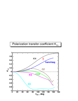
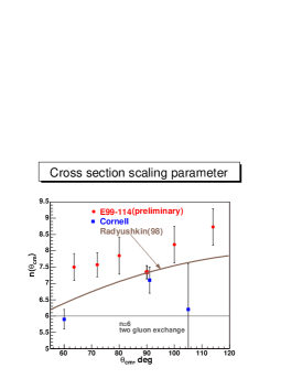
Figure 4: Comparison of preliminary JLab data with theoretical predictions

Furthermore, hard pQCD and soft handbag mechanism give drastically different predictions [10, 14] for the polarization transfer coefficient $K_{LL}$. The preliminary results (Fig. 4, left) of E-99-114 experiment [13] strongly favor handbag mechanism that predicts a value close to the asymmetry for the Compton scattering on a single free quark. Another ratio-type prediction of pQCD is based on the dimensional quark counting rules, which give for WACS $d\sigma/dt\sim s^{-n}f(\theta_{CM})$ with $n=6$ for all center-of-mass angles $\theta_{CM}$. The handbag mechanism corresponds to a power $n$ depending on $\theta_{CM}$, in agreement with the preliminary E-99-114 data [13] (see Fig. 4, right).

4 Distribution amplitudes and pion form factors

Distribution amplitudes describe the hadron structure in situations when pQCD factorization is applicable for exclusive processes. They are defined through matrix elements $\langle 0|\ldots|p\rangle$ of light cone operators. For the pion,

$$\langle\,0\,|\,\bar{\psi}_{d}(-z/2)\gamma_{5}\gamma^{\mu}\psi_{u}(z/2)\,|\,\pi^{+}(p)\,\rangle=ip^{\mu}f_{\pi}\int_{-1}^{1}e^{-i\alpha(pz)/2}\varphi_{\pi}(\alpha)\,d\alpha\,,$$ (5)

with $x_{1}=(1+\alpha)/2,\ x_{2}=(1-\alpha)/2$ being the fractions of the pion momentum carried by the quarks. The simplest case is $\gamma^{*}\gamma\to\pi^{0}$ transition. Its large-$Q^{2}$ behavior is light-cone dominated: there is no competing Feynman-type soft mechanism. The handbag contribution for $\gamma^{*}\gamma\to\pi^{0}$ (Fig. 5, left) is proportional to the $1/(1-\alpha^{2})$ moment of $\varphi_{\pi}(\alpha)$ which allows for an experimental discrimination between the two popular models: asymptotic $\varphi_{\pi}^{as}(\alpha)=\frac{3}{4}(1-\alpha^{2})$ and Chernyak-Zhitnitsky DA $\varphi_{\pi}^{CZ}(\alpha)=\frac{15}{4}\alpha^{2}(1-\alpha^{2})$. Comparison with data favors DA close to $\varphi^{as}_{\pi}(\alpha)$.

Figure 5: Lowest-order pQCD factorization for $\gamma^{*}\gamma\to\pi^{0}$ transition amplitude and for the pion EM form factor.

An important point is that pQCD works here from rather small values $Q^{2}\sim 2\,$GeV², just like in DIS, which is also a purely light-cone dominated process.

Another classic application of pQCD to exclusive processes is the pion electromagnetic form factor. With the asymptotic pion DA, the hard pQCD contribution (Fig. 5, right) to $Q^{2}F_{\pi}(Q^{2})$ is $2\alpha_{s}/\pi\times 0.7\,{\rm GeV}^{2}$, less than 1/3 of experimental value which is close to VMD expectation $1/(1/Q^{2}+1/m_{\rho}^{2})$. The suppression factor $2\alpha_{s}/\pi$ reflects the usual $\alpha_{s}/\pi$ per loop penalty for higher-order corrections. The competing soft mechanism is zero order in $\alpha_{s}$ and dominates over the pQCD hard term at accessible $Q^{2}$. Just like in the case of $F_{1}^{p}(t)$, the soft contribution for $F_{\pi}(Q^{2})$ can be modeled by nonforward parton densities and easily fits the data (see Ref. [15]).

5 Hard electroproduction processes and generalized parton distributions

A more recent attempt to use pQCD to extract information about hadronic structure is the study of deep exclusive photon [2, 3] or meson [3, 16] electroproduction. When both $Q^{2}$ and $s\equiv(p+q)^{2}$ are large while $t\equiv(p-p^{\prime})^{2}$ is small, one can use pQCD factorization of the amplitudes into a convolution of a perturbatively calculable short-distance part and nonperturbative parton functions describing the hadron structure. The hard subprocesses in these two cases have different structure (Fig. 6). For deeply virtual Compton scattering (DVCS), hard amplitude has structure similar to that of the $\gamma^{*}\gamma\pi^{0}$ form factor: the pQCD hard term is of zero order in $\alpha_{s}$, and there is no competing soft contribution. Thus, we can expect that pQCD works from $Q^{2}\sim 2\,{\rm GeV}^{2}$. On the other hand, the deeply virtual meson production process is similar to the pion EM form factor: the hard term has $O(\alpha_{s}/\pi)\sim 0.1$ suppression factor. As a result, the dominance of the hard pQCD term may be postponed to $Q^{2}\sim 5-10\,{\rm GeV}^{2}$.

Figure 6: Hard subprocesses for deeply virtual photon and meson production.

Just like in case of pion and nucleon EM form factors, the competing soft mechanism can mimic the power-law $Q^{2}$-behavior of the hard term. Hence, a mere observation of a “correct” power behavior of the cross section is not a proof that pQCD is already working. One should look at several characteristics of the reaction to make conclusions about the reaction mechanism.

To visualize DVCS’s specifics, take the $\gamma^{*}N$ center-of-mass frame, with the initial hadron and the virtual photon moving in opposite directions along the $z$-axis. Since $t$ is small, the hadron and the real photon in the final state also move close to the $z$-axis. This means that the virtual photon momentum $q=q^{\prime}-x_{Bj}p$ (where $x_{Bj}={Q^{2}}/{2(pq)}$ is the same Bjorken variable as in DIS) has the component $-x_{Bj}p$ canceled by the momentum transfer $r$. In other words, $r$ has the longitudinal component $r^{+}=x_{Bj}p^{+}$, and DVCS has skewed kinematics: the final hadron’s “plus” momentum $(1-\zeta)p^{+}$ is smaller than that of the initial hadron (for DVCS, $\zeta=x_{Bj}$). The plus-momenta $Xp^{+}$ and $(X-\zeta)p^{+}$ of the initial and final quarks in DVCS are also not equal. Furthermore, the invariant momentum transfer $t$ in DVCS is nonzero. Thus, the nonforward parton distributions (NFPDs) ${\mathcal{F}}_{\zeta}(X;t)$ describing the hadronic structure in DVCS depend on $X$, the fraction of $p^{+}$ carried by the initial quark, on $\zeta$, the skewness parameter characterizing the difference between initial and final hadron momenta, and on $t$, the invariant momentum transfer. In the forward $r=0$ limit, we have a reduction formula ${\mathcal{F}}^{a}_{\zeta=0}(X,t=0)=f_{a}(X)$ relating NFPDs with the usual parton densities. The nontriviality of this relation is that ${\mathcal{F}}_{\zeta}(X;t)$ appear in the amplitude of the exclusive DVCS process, while the usual parton densities are extracted from the cross section of the inclusive DIS reaction. In the limit of zero skewness, NFPDs correspond to nonforward parton densities ${\mathcal{F}}^{a}_{\zeta=0}(X,t)={\mathcal{F}}^{a}(X,t)$. The local limit results in a formula similar to Eq.(3) : $X$ integral of ${\mathcal{F}}^{a}_{\zeta}(X,t)-{\mathcal{F}}^{\bar{a}}_{\zeta}(X,t)$ gives $F_{1a}(t)$.

The NFPD convention uses the variables most close to those of the usual parton densities. To treat initial and final hadron momenta symmetrically, Ji proposed [2] the variables in which the plus-momenta of the hadrons are $(1+\xi)P^{+}$ and $(1-\xi)P^{+}$, and those of the active partons are $(x+\xi)P^{+}$ and $(x-\xi)P^{+}$, with $P=(p+p^{\prime})/2$ (Fig. 7). Since $\zeta p^{+}=r^{+}=2\xi P^{+}$, we have $\xi=\zeta/(2-\zeta)$. To take into account spin properties of hadrons and quarks, one needs 4 off-forward parton distributions $H,E,\tilde{H},\widetilde{E}$, all being functions of $x,\xi,t$. Each OFPD has 3 distinct regions. When $\xi<x<1$, it is analogous to usual quark distributions; when $-1<x<-\xi$, it is similar to antiquark distributions. In the region $-\xi<x<\xi,$ the “returning” quark has negative plus-momentum, and should be treated as an outgoing antiquark with momentum $(\xi-x)P^{+}$. The total $q\bar{q}$ pair momentum $r^{+}=2\xi P^{+}$ is shared by the quarks in fractions $r^{+}(1+x/\xi)/2$ and $r^{+}(1-x/\xi)/2$. Hence OFPD in this region $-\xi<x<\xi$ is similar to a distribution amplitude $\Phi(\alpha)$ with $\alpha=x/\xi$. In the local limit, OFPDs reduce to form factors

Figure 7: Comparison of NFPDs and OFPDs.

$$\sum_{a}e_{a}\int\limits_{-1}^{1}{H}^{a}(x,\xi;t)\,dx=F_{1}(t)\ \ ,\ \sum_{a}e_{a}\int\limits_{-1}^{1}{E}^{a}(x,\xi;t)\,dx=F_{2}(t)\ .$$ (6)

The $E$ function, like $F_{2}$, comes with the $r_{\mu}$ factor, hence, it is invisible in DIS described by exactly forward $r=0$ Compton amplitude. However, the limit $E^{a,\bar{a}}(x,\xi=0;t=0)\equiv\kappa^{a,\bar{a}}(x)$ exists. These functions give the proton anomalous magnetic moment $\kappa_{p}$, and, through Ji’s sum rule [2], the total quark contribution $J_{q}$ into the proton spin

$$\kappa_{p}=\sum_{a}e_{a}\int\limits_{0}^{1}(\kappa^{a}(x)-\kappa^{\bar{a}}(x))\,dx\ ,$$ (7)

$$J_{q}=\frac{1}{2}\sum_{a}\int\limits_{0}^{1}x\,[f^{a}(x)+f^{\bar{a}}(x)+\kappa^{a}(x)+\kappa^{\bar{a}}(x)]\,dx\ .\ \$$ (8)

Only valence quarks contribute to $\kappa_{p}$, while $J_{q}$ involves also sea quarks. The determination of the $\kappa$-contribution to Ji’s sum rule is one of the original motivations [2] to study the GPDs.

6 Double distributions

To model GPDs, two approaches are used: a direct calculation in specific dynamical models (bag model, chiral soliton model, light-cone formalism, etc.) and phenomenological construction based on the relation of SPDs to usual parton densities $f_{a}(x),\Delta f_{a}(x)$ and form factors $F_{1}(t),F_{2}(t),G_{A}(t),G_{P}(t)$. The key question is the interplay between $x,\xi$ and $t$ dependencies of GPDs. There are not so many cases in which the pattern of the interplay is evident. One example is the function $\widetilde{E}(x,\xi;t)$ that is related to $G_{P}(t)$ form factor and is dominated for small $t$ by the pion pole term $1/(t-m_{\pi}^{2})$. It is also proportional to the pion distribution amplitude $\varphi(\alpha)\approx\frac{3}{4}f_{\pi}(1-\alpha^{2})$ taken at $\alpha=x/\xi$. The construction of self-consistent models for other GPDs is performed using the formalism of double distributions [1, 3, 17].

The main idea behind the double distributions is a “superposition” of $P^{+}$ and $r^{+}$ momentum fluxes, i.e., the representation of the parton momentum $k^{+}=\beta P^{+}+(1+\alpha)r^{+}/2$ as the sum of a component $\beta P^{+}$ due to the average hadron momentum $P$ (flowing in the $s$-channel) and a component $(1+\alpha)r^{+}/2$ due to the $t$-channel momentum $r$. Thus, the double distribution $f(\beta,\alpha)$ (we consider here for simplicity the $t=0$ limit) looks like a usual parton density with respect to $\beta$ and like a distribution amplitude with respect to $\alpha$ (Fig. 8). Using $r^{+}=2\xi P^{+}$ gives the connection $x=\beta+\xi\alpha$ between DD variables $\beta,\alpha$ and OFPD variables $x,\xi$.

Figure 8: Comparison of GPD and DD descriptions.

The forward limit $\xi=0,t=0$ corresponds to $x=\beta$, and gives the relation between DDs and the usual parton densities

$$\int_{-1+|\beta|}^{1-|\beta|}f_{a}(\beta,\alpha;t=0)\,d\alpha=f_{a}(\beta)\ .$$ (9)

The DDs live on the rhombus $|\alpha|+|\beta|\leq 1$ and they are symmetric functions of the “DA” variable $\alpha$: $f_{a}(\beta,\alpha;t)=f_{a}(\beta,-\alpha;t)$ (“Munich” symmetry [18]). These restrictions suggest a factorized representation for a DD in the form of a product of a usual parton density in the $\beta$-direction and a distribution amplitude in the $\alpha$-direction. In particular, a toy model for a double distribution

$$f(\beta,\alpha)=3[(1-|\beta|)^{2}-\alpha^{2}]\,\theta(|\alpha|+|\beta|\leq 1)$$

corresponds to the toy “forward” distribution $f(\beta)=4(1-|\beta|)^{3}$, and the $\alpha$-profile like that of the asymptotic pion distribution amplitude.

To get usual parton densities from DDs, one should integrate (scan) them over vertical lines $\beta=x={\rm const}$. To get OFPDs $H(x,\xi)$ with nonzero $\xi$ from DDs $f(\beta,\alpha)$, one should integrate (scan) DDs along the parallel lines $\alpha=(x-\beta)/\xi$ with a $\xi$-dependent slope. One can call this process the DD-tomography. The basic feature of OFPDs $H(x,\xi)$ resulting from DDs is that for $\xi=0$ they reduce to usual parton densities, and for $\xi=1$ they have a shape like a meson distribution amplitude.

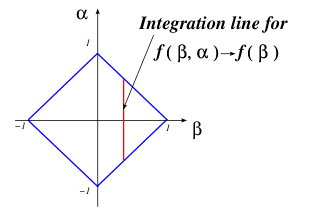
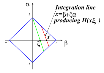
Figure 9: Scanning pattern for DD $\to$ SPD conversion

In fact, such a DD modeling misses terms proportional to the momentum transfer, and thus invisible in the forward limit. These include meson exchange contributions and so-called D-term, which can be interpreted as $\sigma$-exchange. The inclusion of the D-term induces nontrivial behavior in the central $|x|<\xi$ region (for details, see Ref. [4]).

7 Conclusions

Hadronic structure is a complicated subject, it requires a study from many sides, in many different types of experiments. The description of specific aspects of hadronic structure is provided by several different functions: form factors, usual parton densities, distribution amplitudes. Generalized parton distributions provide a unified description: all these functions can be treated as particular or limiting cases of GPDs $H(x,\xi,t)$.

Usual Parton Densities $f(x)$ correspond to the case $\xi=0,t=0$. They describe a hadron in terms of probabilities $\sim|\Psi|^{2}$. But QCD is a quantum theory: GPDs with $\xi\neq 0$ describe correlations $\sim\Psi_{1}^{*}\Psi_{2}$. Taking only one point $t=0$ corresponds to integration over impact parameters $b_{\perp}$ - information about the transverse structure is lost.

Form Factors $F(t)$ contain information about the distribution of partons in the transverse plane, but $F(t)$ involve integration over momentum fraction $x$ - information about longitudinal structure is lost.

Nonforward parton densities. A simple “hybridization” of usual densities and form factors in terms of NPDs ${\mathcal{F}}(x,t)$ (GPDs with $\xi=0$) shows that behavior of $F(t)$ is governed both by transverse and longitudinal distributions. NPDs provide adequate description of nonperturbative soft mechanism, they also allow to study transition from soft to hard mechanism.

Distribution Amplitudes $\varphi(x)$ provide quantum level information about longitudinal structure of hadrons. Information about DAs is accessible in hard exclusive processes, when asymptotic pQCD mechanism dominates. GPDs have DA-type structure in the central region $|x|<\xi$.

Generalized Parton Distributions $H(x,\xi;t)$ provide a 3-dimensional picture of hadrons. GPDs also provide some novel possibilities, such as “magnetic distributions” related to the spin-flip GPDs $E_{a}(x,\xi,t)$. In particular, the structure of the nonforward density ${\mathcal{E}}_{a}(x,t)\equiv E_{a}(x,\xi=0,t)$ determines the $t$-dependence of $F_{2}(t)$. Recent JLab data on the ratio $F_{2}(t)/F_{1}(t)$ can be explained within a GPD-based model [8] by assuming an extra $(1-x)^{\eta}$ suppression of ${\mathcal{E}}(x,t)$. The forward reductions $\kappa^{a}(x)$ of $E_{a}(x,\xi,t)$ look as fundamental as $f^{a}(x)$ and $\Delta f^{a}(x)$: Ji’s sum rule involves $\kappa^{a}(x)$ on equal footing with $f^{a}(x)$. Magnetic properties of hadrons are strongly sensitive to dynamics, thus providing a testing ground for models.

A new direction is the study of flavor-nondiagonal distributions: proton-to-neutron GPDs accessible through exclusive charged pion electroproduction process, proton-to-$\Lambda$ GPDs (they appear in kaon electroproduction); proton-to-Delta – this one can be related to form factors of $p\Delta^{+}$ transition (another puzzle for hard pQCD approachable by the NPD model [8]). The GPDs for $N\to N+{\rm soft}\ \pi$ processes [4] can be used for testing the soft pion theorems and physics of chiral symmetry breaking.

A challenging problem is the separation and flavor decomposition of GPDs. The DVCS amplitude involves all 4 types: $H,E,\widetilde{H},\widetilde{E}$ of GPDs, so we need to study other processes involving different combinations of GPDs. An important observation is that, in hard electroproduction of mesons, the spin nature of the produced meson dictates the type of GPDs involved, e.g., for pion electroproduction, only $\widetilde{H},\widetilde{E}$ appear, with $\widetilde{E}$ dominated by the pion pole at small $t$. This gives access to (generalization of) polarized parton densities without polarizing the target.

8 Acknowledgements

I thank the organizers for invitation, support and hospitality in Minneapolis. This work is supported by the US Department of Energy contract DE-AC05-84ER40150 under which the Southeastern Universities Research Association (SURA) operates the Thomas Jefferson Accelerator Facility.

References

- [1] D. Muller, D. Robaschik, B. Geyer, F. M. Dittes and J. Horejsi, Fortsch. Phys. 42, 101 (1994).
- [2] X. D. Ji, Phys. Rev. Lett. 78, 610 (1997), Phys. Rev. D 55, 7114 (1997).
- [3] A. V. Radyushkin, Phys. Lett. B 380, 417 (1996), Phys. Lett. B 385, 333 (1996), Phys. Rev. D 56, 5524 (1997).
- [4] K. Goeke, M. V. Polyakov and M. Vanderhaeghen, Prog. Part. Nucl. Phys. 47, 401 (2001).
- [5] M. Diehl, Phys. Rept. 388, 41 (2003)
- [6] A. V. Radyushkin, Phys. Rev. D 58, 114008 (1998).
- [7] V. Barone, M. Genovese, N. N. Nikolaev, E. Predazzi and B. G. Zakharov, Z. Phys. C 58, 541 (1993).
- [8] M. Guidal, M. V. Polyakov, A. V. Radyushkin and M. Vanderhaeghen, in preparation (2004).
- [9] O. Gayou et al. [Jefferson Lab Hall A Collaboration], Phys. Rev. Lett. 88, 092301 (2002) [arXiv:nucl-ex/0111010].
- [10] M. Diehl, T. Feldmann, R. Jakob and P. Kroll, Eur. Phys. J. C 8, 409 (1999).
- [11] A. Shupe et al., Phys. Rev. D 19, 1921 (1979).
- [12] A. Nathan, “Real Compton scattering from the proton”, in “Exclusive processes at high momentum transfer”, World Scientific, Singapore, (2002) pp. 225-232.
- [13] B. Wojtsekhowski, private communication (2004).
- [14] T. C. Brooks and L. J. Dixon, Phys. Rev. D 62, 114021 (2000) [arXiv:hep-ph/0004143].
- [15] A. Mukherjee, I. V. Musatov, H. C. Pauli and A. V. Radyushkin, Phys. Rev. D 67, 073014 (2003) [arXiv:hep-ph/0205315].
- [16] J. C. Collins, L. Frankfurt and M. Strikman, Phys. Rev. D 56, 2982 (1997).
- [17] A. V. Radyushkin, Phys. Rev. D 59, 014030 (1999).
- [18] L. Mankiewicz, G. Piller and T. Weigl, Eur. Phys. J. C 5, 119 (1998).