Higgs Phenomenology in the
Two Higgs Doublet Model of type II
A dissertation submitted to
the University of San Francisco-Quito
in partial fulfillment of
the requirements for the degree of
Doctor of Philosophy

Abstract

We calculate the rate of $\pi^{+}$, $K^{+}$, $D^{+}$ and $B^{+}\rightarrow\mu^{+}\nu_{\mu}$ decays, the branching ratio corresponding to $H^{+}\rightarrow\tau^{+}\nu_{\tau}$, and the box diagrams of $B^{o}\leftrightarrow\bar{B}^{o}$, $K^{o}\leftrightarrow\bar{K}^{o}$ and $D^{o}\leftrightarrow\bar{D}^{o}$ mixing in the Two Higgs Doublet Model (Model II). Using the experimental data on meson decay rates, mixing, and CP violation in the $K^{o}$ and $B^{o}$ systems we set competitive upper and lower limits to the parameter $\tan\beta$ as a function of the mass of the charged Higgs $m_{H}$.

Abstract

We calculate masses, production cross sections, and decay rates in the Two Higgs Doublet Model of type II. We also discuss running coupling constants and Grand Unification. The most interesting production channels are $gg\rightarrow h^{0},H^{0},A^{0}$ on mass shell, and $q\bar{q},gg\rightarrow h^{0}Z$ and $q\bar{q^{\prime}}\rightarrow h^{0}W^{\pm}$ in the continuum (tho there may be peaks at $m_{A^{0}}$). The most interesting decays are $h^{0},H^{0},A^{0}\rightarrow b\bar{b}$-jets and $\tau^{+}\tau^{-}$, and, if above threshold, $H^{0}\rightarrow ZZ$, $W^{+}W^{-}$ and $h^{0}h^{0}$. The following final states should be compared with the Standard Model cross section: $b\bar{b}Z$, $b\bar{b}W^{\pm}$, $\tau^{+}\tau^{-}Z$, $\tau^{+}\tau^{-}W^{\pm}$, $b\bar{b}$, $\tau^{+}\tau^{-}$, $ZZ$, $W^{+}W^{-}$, 3 and 4 $b$-jets, $2\tau^{+}+2\tau^{-}$, $b\bar{b}\tau^{+}\tau^{-}$, $ZW^{+}W^{-}$, $3Z$, $ZZW^{\pm}$ and $3W^{\pm}$. Mass peaks should be searched in the following channels: $Zb\bar{b}$, $ZZ$, $ZZZ$, $b\bar{b}$, $4b$-jets and, just in case, $Z\gamma$.

Abstract

We calculate Higgs production cross sections at a muon collider in the Two Higgs Doublet Model of type II. The most interesting productions channels are $\mu^{-}\mu^{+}\rightarrow h^{0}Z^{0},H^{0}Z^{0},H^{-}H^{+},A^{0}Z^{0}$ and $H^{\mp}W^{\pm}$. The last channel is compared with the production processes $p\bar{p}\rightarrow H^{\mp}W^{\pm}X$ and $pp\rightarrow H^{\mp}W^{\pm}X$ at the Tevatron and LHC energies, respectively, for large values of $\tan\beta$.

Chapter 1 Introduction

The Standard Model of quarks and leptons is based on some basic principles: special relativity, locality, quantum mechanics, local symmetries and renormalizability [1]. Therefore the predictions of the Standard Model “are precise and unambiguous, and generally cannot be modified ‘a little bit’ except in very limited specific ways. This feature makes the experimental success especially meaningful, since it becomes hard to imagine that the theory could be approximately right without in some sense being exactly right.”[1] The Standard Model predicts the existence of a massive spin zero boson called Higgs particle. The Higgs mechanism is responsible for the masses of the weak interaction gauge bosons $W^{\pm}$ and $Z^{0}$, and is also sufficient to give masses to the leptons and quarks. The discovey of the Standard Model Higgs is then one of the principal goals of experimental and theoretical particle physicists. We could say that the Higgs mechanism is a cornerstone of the Standard Model.

Among the extensions of the Standard Model that respect its principles and symmetries, that are compatible with present data within a region of parameter space, and are of interest at the large particle colliders, is the addition of a second doublet of Higgs fields. Higgs doublets can be added to the Standard Model without upsetting the $Z/W$ mass ratio; higher dimensional representations upset this ratio [2].

In the Two Higgs Doublet Model there are two choices for the Higgs-quark interactions. In Model I, the quarks and leptons do not couple to the first Higgs doublet ($\Phi_{1}$), but couple to the second Higgs doublet ($\Phi_{2}$). In Model II, $\Phi_{1}$ couples only to down-type quarks and leptons and $\Phi_{2}$ couples only to up-type quarks and neutrinos. If we consider the neutrinos as massless particles, there are no couplings between neutrinos and neutral Higgs bosons. The Model II choice for the Higgs-fermion couplings is the required structure for the Minimal Supersymmetric Model.

After the electroweak symmetry-breaking mechanism, three of the eight degrees of freedom are absorbed by the $W^{\pm}$ and $Z^{0}$ gauge bosons, leading to the existence of five elementary Higgs particles. The physical spectrum of the Two Higgs Doublet Model (Model II) contains five Higgs bosons: one pseudoscalar $A^{0}$ (CP-odd scalar), two neutral scalars $H^{0}$ and $h^{0}$ (CP-even scalars), and two charged scalars $H^{+}$ and $H^{-}$. In the most general model, the masses of the Higgs bosons, the mixing angle $\alpha$ $(-\pi/2<\alpha\leq 0)$ between the two neutral scalar Higgs fields, and the ratio of the vacuum expectation values of the two neutral components of the Higgs doublets, $\tan\beta$ ($0\leq\beta<\frac{\pi}{2}$), are all independent parameters of the theory [3]. However, in the Minimal Supersymmetric Model the conditions on the potential imposed by supersymmetry reduces the number of parameteres to two, which may be chosen to be $\tan\beta$ and $m_{H}$ [3].

$$\Phi_{1}=\left(\begin{array}[]{c}\Phi_{1}^{o*}\\ -\Phi_{1}^{-}\end{array}\right),\qquad\Phi_{2}=\left(\begin{array}[]{c}\Phi_{2}^{+}\\ \Phi_{2}^{o}\end{array}\right),\qquad\tan\beta\equiv\frac{\langle\Phi_{2}^{o}\rangle}{\langle\Phi_{1}^{o*}\rangle}.$$

In this thesis we study the Two Higgs Doublet Model of type II, set limits to the parameter $\tan\beta$ as a function of the mass of the charged Higgs $m_{H}$, and find interesting discovery channels in hadron colliders or muon colliders.

All the analysis in this thesis are based on the “tree-level Higgs potential” [3].

The plan in my thesis is the following:

In the second Chapter[4], using the experimental data on meson decay rates, mixing and CP violation in the $K^{0}$ and $B^{0}$ systems, we set limits to the parameter $\tan\beta$ as a function of the mass of the charged Higgs $m_{H}$. Recent measurements of $\sin(2\beta_{CKM})$ by the B-factories Belle [5] and BaBar [6] permit us to set more stringent limits on $\tan\beta$. $\beta_{CKM}$ is an angle of the “unitarity triangle”. [7]

In the third Chapter[8], we present graphically the corresponding limits on $m_{H^{0}}$, $m_{h^{0}}$ and $m_{A^{0}}$ as a function of the mass of the charged Higgs, without considering the influence of radiative corrections. Then we calculate production cross sections, decay rates and branching fractions of the Higgs particles. Next, we obtain the running coupling constants and discuss Grand Unification. Finally, in the Conclusions, we list interesting discovery channels.

In Chapter four [9], we analyze the possibility of the construction of a $\mu^{-}\mu^{+}$ collider to detect charged or neutral Higgs bosons. The reason for this is that in a muon collider, the signal could be cleaner than in a hadron collider. Some of the production cross sections that we study are: $\mu^{-}\mu^{+}\rightarrow h^{0}Z^{0},H^{0}Z^{0},H^{-}H^{+},A^{0}Z^{0}$ and $H^{\mp}W^{\pm}$. Then, we compare the channel $\mu^{-}\mu^{+}\rightarrow H^{\mp}W^{\pm}$ (at $\sqrt{s}=500\textrm{GeV/c}$ and for large values of $\tan\beta$) with the production processes $p\bar{p}\rightarrow H^{\mp}W^{\pm}X$ (at the Tevatron) and $pp\rightarrow H^{\mp}W^{\pm}X$ (at the LHC), taking into account the $t\bar{t}$ background, to check the feasibility of detecting $H^{\pm}$ using a muon collider. The influence of radiative corrections in the masses of the Higgs bosons is considered in all the calculations. Finally, in the Conclusions, we also check the process $\mu^{-}\mu^{+}\rightarrow A^{0}h^{0}$.

$\bf{NOTE:}$ The results presented in this thesis (width decays, production cross sections, etc.) are calculated in detail in reference [10].

Chapter 2 Limits on the Two Higgs Doublet Model from meson decay, mixing and CP violation

2.1 Introduction

The Standard Model of quarks and leptons is here to stay. This theory is based on principles: special relativity, locality, quantum mechanics, local symmetries and renormalizability[1]. Therefore the predictions of the Standard Model “are precise and unambiguous, and generally cannot be modified ‘a little bit’ except in very limited specific ways. This feature makes the experimental success especially meaningful, since it becomes hard to imagine that the theory could be approximately right without in some sense being exactly right.”[1] Among the extensions of the Standard Model that respect its principles and symmetries, that are compatible with present data within a region of parameter space, and are of interest at the large particle colliders, is the addition of a second doublet of Higgs fields. Higgs doublets can be added to the Standard Model without upsetting the $Z/W$ mass ratio; higher dimensional representations upset this ratio. A second Higgs doublet could make the three running coupling constants of the Standard Model meet at the Grand Unified Theory (GUT) scale. A second Higgs doublet is necessary in Supersymmetric extensions of the Standard Model[2]. In this article we explore the limits that present data place on the parameters of the Two Higgs Doublet Model (Model II).[3] In particular we consider meson decay, mixing and CP violation.

All of our analysis is based on the “tree-level Higgs potential”[3]. The physical spectrum of the Two Higgs Doublet Model (Model II) contains five Higgs bosons: one pseudoscalar $A^{o}$ (CP-odd scalar), two neutral scalars $H^{o}$ and $h^{o}$ (CP-even scalars), and two charged scalars $H^{+}$ and $H^{-}$. In the most general model, the masses of the Higgs bosons, the mixing angle $\alpha$ between the two neutral scalar Higgs fields, and the ratio of the vacuum expectation values of the two neutral components of the Higgs doublets, $\tan\beta>0$, are all independent parameters of the theory. However, in the Minimal Supersymmetric Model the conditions on the potential imposed by supersymmetry reduces the number of parameters to two, which may be chosen to be $\tan\beta$ and $m_{H}$ [3].

$$\Phi_{1}=\left(\begin{array}[]{c}\Phi_{1}^{o*}\\ -\Phi_{1}^{-}\end{array}\right),\qquad\Phi_{2}=\left(\begin{array}[]{c}\Phi_{2}^{+}\\ \Phi_{2}^{o}\end{array}\right),\qquad\tan\beta\equiv\frac{\langle\Phi_{2}^{o}\rangle}{\langle\Phi_{1}^{o*}\rangle}.$$

Using the experimental data on meson decay rates, mixing and CP violation we set limits to the parameter $\tan\beta$ as a function of the mass of the charged Higgs $m_{H}$. Recent measurements of $\sin(2\beta_{CKM})$ by the B-factories Belle[5] and BaBar[6] permit us to set more stringent limits on $\tan\beta$. $\beta_{CKM}$ is an angle of the “unitarity triangle”.[7]

2.2 Feynman rules of the charged Higgs in the Two Higgs Doublet Model.

The effective Lagrangian corresponding to the $H^{\pm}f\bar{f}^{\prime}$ vertex is:

$$\mathcal{L}_{H^{\pm}ff^{\prime}} = \frac{g}{2\sqrt{2}m_{W}}\{H^{+}V_{ff^{\prime}}\bar{u}_{f}\left(A+B\gamma^{5}\right)v_{\bar{f}^{\prime}}$$ (2.2)

$$+H^{-}V_{ff^{\prime}}^{*}\bar{u}_{f^{\prime}}(A-B\gamma^{5})v_{\bar{f}}\}$$

where

$$A\equiv\left(m_{f^{\prime}}\tan\beta+m_{f}cot\beta\right)$$ (2.3)

and

$$B\equiv\left(m_{f^{\prime}}\tan\beta-m_{f}cot\beta\right),$$ (2.4)

$f=$ fermion (quark or lepton) and $\bar{f^{\prime}}=$ antifermion (antiquark or antilepton). $V_{ff^{\prime}}$ is an element of the CKM matrix.

The charged-Higgs propagator is: $i/\left(\mathrm{K}^{2}-m_{H}^{2}+i\varepsilon\right)$.

2.3 Theory

Consider the $\left(B^{o},\bar{B}^{o}\right)$ system. $B^{o}\leftrightarrow\bar{B}^{o}$ mixing occurs because of the box diagrams illustrated in Figure 2.1. The difference in mass of the two eigenstates that diagonalize the hamiltonian can be written in the form

$$\Delta m_{B}=\frac{\beta_{B}G_{F}^{2}m_{W}^{2}f_{B}^{2}m_{B}}{6\pi^{2}}$$ (2.5)

$$\times\left|\sum_{i,j}\xi_{i}\xi_{j}\left[S^{WW}-2\cot^{2}\beta\cdot S^{HW}+\frac{1}{4}\cot^{4}\beta\cdot S^{HH}\right]\right|.$$

The functions

$$S^{WW}\left(x_{W}^{i},x_{W}^{j}\right),\textrm{ }S^{HW}\left(x_{W}^{i},x_{W}^{j},x_{H}^{i},x_{H}^{j},x_{H}^{W}\right)\textrm{ and }S^{HH}\left(x_{H}^{i},x_{H}^{j},x_{H}^{W}\right)$$

are obtained from the box diagrams and are written in Appendix A. The Feynman rules for $H^{\pm}$ are listed in Section 2.2. We have derived[8] $S^{WW}$ in agreement with the literature[9]. The derivation of $S^{HW}$ and $S^{HH}$ is given in Appendices B and C [10]. The variables of these functions are

$$x_{W}^{i}\equiv\frac{m_{i}^{2}}{m_{W}^{2}},\qquad x_{H}^{i}\equiv\frac{m_{i}^{2}}{m_{H}^{2}},\qquad\textrm{and}\qquad x_{H}^{W}\equiv\frac{m_{W}^{2}}{m_{H}^{2}}$$

where $i=u,c,t$. $\xi_{i}\equiv V_{ib}V_{id}^{*}$. The notation for the remaining symbols in (2.5) is standard[7]. To obtain the Standard Model[9], omit $S^{HW}$ and $S^{HH}$. $\beta_{B}$ is a factor of order 1. Estimates of $\beta_{B}$ using “vacuum intermediate state insertion”[9], “PCAC and vacuum saturation”[9], “bag model”[9], “QCD corrections”[11, 12], and the “free particles in a box”[8] models span the range $\approx 0.4$ to $\approx 1$. $f_{B}$ is the decay constant that appears in the decay rate for $B^{+}\rightarrow\mu^{+}\nu_{\mu}$[7] which at tree level in the Two Higgs Doublet Model (Model II) is:

Figure 2.1: Feynman diagrams corresponding to $B^{o}\leftrightarrow\bar{B}^{o}$ mixing in the Two Higgs Doublet Model. $q=d$ or $s$ and $i,j=u,c,t$. The diagrams on the right side interfer with a “-” sign.

$$\Gamma_{B^{+}}=\frac{\mathopen{|}V_{ub}\mathclose{|}^{2}}{8\pi}G_{F}^{2}m_{\mu}^{2}m_{B^{+}}\left(1-\frac{m_{\mu}^{2}}{m_{B^{+}}^{2}}\right)^{2}\left[f_{B}-g_{B}\frac{m_{B^{+}}^{2}}{m_{H}^{2}}\tan^{2}\beta\right]^{2}$$ (2.6)

In the derivation of (2.6) we have substituted

$$\bar{v}\left(\bar{\textrm{b}}\right)\gamma^{\mu}\left(1-\gamma^{5}\right)u\left(\textrm{u}\right)\rightarrow p^{\mu}f_{B},$$

$$\bar{v}\left(\bar{\textrm{b}}\right)\left(1-\gamma^{5}\right)u\left(\textrm{u}\right)\rightarrow-\frac{m_{B^{+}}^{2}}{m_{b}}g_{B}$$

which defines the decay constants $f_{B}$ and $g_{B}$. $\bar{v}\left(\bar{\textrm{b}}\right)$ and $u\left(\textrm{u}\right)$ are spinors, see Section 2. We expect $f_{B}\approx g_{B}$: for a scalar meson with the quark and antiquark at rest $f_{B}=\frac{m_{B^{+}}}{m_{b}}g_{B}$. The decays $B^{+}\rightarrow\mu^{+}\nu_{\mu}$ and $D^{+}\rightarrow\mu^{+}\nu_{\mu}$ are not yet accessible to experiment so that $f_{B}$ and $f_{D}$ are unknown. $f_{B}$ is estimated using sum rules[13], or the $B^{*}-B$ mass difference[14], or a phenomenological model[15], or the MIT bag model[16]. These estimates span the range $\approx 0.06\mathrm{GeV}$ to $\approx 0.2\mathrm{GeV}$ with the convention used in reference [7] and in Equation (2.6).

In the “free particles in a box”[8] model $\beta_{B}=1$ (after correcting [8] by a color factor $4/3$) and the volume of the box, i.e. the meson, is $V=8/\left(\beta_{B}m_{B}f_{B}^{2}\right)$.

For the $\left(B_{s}^{o},\bar{B}_{s}^{o}\right)$ system: $\xi_{i}\equiv V_{ib}V_{is}^{*}$ where $i=u,c,t$; in (2.5) replace subscript $B$ by $B_{s}$. For the $\left(K^{o},\bar{K}^{o}\right)$ system: $\xi_{i}\equiv V_{is}V_{id}^{*}$ where $i=u,c,t$; in (2.5) replace subscript $B$ by $K$. The CP violation parameter $\varepsilon$[9, 7] in the $\left(K^{o},\bar{K}^{o}\right)$ system in the Two Higgs Doublet Model is given by:

$$\varepsilon=e^{i\frac{\pi}{4}}\cdot\frac{Im\left(\sum_{i,j}\xi_{i}\xi_{j}\left[S^{WW}-2\cot^{2}\beta\cdot S^{HW}+\frac{1}{4}\cot^{4}\beta\cdot S^{HH}\right]\right)}{2\sqrt{2}\cdot\left|\sum_{i,j}\xi_{i}\xi_{j}\left[S^{WW}-2\cot^{2}\beta\cdot S^{HW}+\frac{1}{4}\cot^{4}\beta\cdot S^{HH}\right]\right|}$$ (2.7)

For the $\left(D^{o},\bar{D}^{o}\right)$ system: $\xi_{i}\equiv V_{ci}V_{ui}^{*}$ where $i=d,s,b$; in (2.5) replace subscript $B$ by $D$ and replace $\cot\beta$ by $\tan\beta$ (leave $\tan\beta$ as is in (2.6)).

The branching ratio for $H^{+}\rightarrow\tau^{+}\nu_{\tau}$ for $m_{H}<m_{t}$ is given by

$$B\left(H^{+}\rightarrow\tau^{+}\nu_{\tau}\right)\approx\\ \frac{m_{\tau}^{2}\tan^{2}\beta}{\left|V_{cs}\right|^{2}a+\left|V_{cb}\right|^{2}b+m_{\tau}^{2}\tan^{2}\beta}$$ (2.8)

with $a\equiv 3\left[m_{s}^{2}\tan^{2}\beta+m_{c}^{2}\cot^{2}\beta\right]$ and $b\equiv 3\left[m_{b}^{2}\tan^{2}\beta+m_{c}^{2}\cot^{2}\beta\right]$. From the measured limit[17] on $m_{H}$ as a function of the branching ratio and (2.8) we obtain a lower bound of $m_{H}$ for each $\tan\beta$.

Let us finally mention that the time-dependent CP-violating asymmetry $A\equiv(\Gamma-\bar{\Gamma})/(\Gamma+\bar{\Gamma})$, where $\Gamma$ ($\bar{\Gamma}$) is the rate of the decay $B^{o}\rightarrow J/\psi+K_{s}$ ($\bar{B^{o}}\rightarrow J/\psi+K_{s}$), measured by CDF, Belle and BaBar is given by $\sin(2\beta_{CKM})\cdot\sin(\Delta Mt)$ in both the Standard Model and in the Two Higgs Doublet Model (Model II). This is because the dominating terms of $\xi_{i}\xi_{j}S^{HW}$ and $\xi_{i}\xi_{j}S^{HH}$ have $i=j=t$.

2.4 Limits

All experimental data are taken from [7]. In order to obtain limits we assume conservatively $0.4<\beta_{x}<1.8$, and $f_{x}=g_{x}$ with $x=B$, $B_{s}$, $D$, $K$, $\pi$. These assumptions are not critical since the upper (lower) limits on $\tan\beta$ depend on terms $\propto\tan^{4}\beta$ ($\propto\cot^{4}\beta$) in (2.5) or (2.6). We take the magnitude of the elements of the CKM matrix from [7] and leave the phase $\angle V_{ub}$ as a free parameter. The following calculations are made for each $(m_{H},\tan\beta)$. The measured value of the parameter $\varepsilon$ determines the phase $\angle V_{ub}$ of the CKM matrix, and hence $\beta_{CKM}$. This phase is required to be within the experimental bounds: $0.325<\tan(\beta_{CKM})<0.862$ at $95\%$ confidence level [7]. The measured decay rates $\Gamma_{K}$ and $\Gamma_{\pi}$ determine $f_{K}$ and $f_{\pi}$ using (2.6). The experimental upper bounds on $\Gamma_{B}$ and $\Gamma_{D}$ determine upper bounds on $f_{B}$ and $f_{D}$ using (2.6). The measured $\Delta m_{B}$ and $\Delta m_{K}$ determine $\beta_{B}f_{B}^{2}$ and $\beta_{K}f_{K}^{2}$ using (2.5). The experimental upper bound on $\Delta m_{D}$ determines an upper bound on $\beta_{D}f_{D}^{2}$. The experimental lower bound on $\Delta m_{Bs}$ determines a lower bound on $\beta_{Bs}f_{Bs}^{2}$. From the preceding information we obtain $\beta_{K}$ and a lower bound on $\beta_{B}$. Then the requirements $0.4<\beta_{K}<1.8$, $\beta_{B}<1.8$ and $0.325<\tan(\beta_{CKM})<0.862$ place limits on $\tan\beta$ for each $m_{H}$ as listed in Table 2.1. The confidence level of these limits is $95\%$. It turns out that the lower limit on $\tan\beta$ is determined by the experimental lower limit of $\tan(\beta_{CKM})$, and the upper limit on $\tan\beta$ is determined by $\beta_{B}<1.8$.

$m_{H}=100$GeV	$1.74$ $<\tan\beta<67$
$m_{H}=200$GeV	$1.36$ $<\tan\beta<134$
$m_{H}=300$GeV	$1.13$ $<\tan\beta<202$
$m_{H}=1000$GeV	$0.58$ $<\tan\beta<672$

Table 2.1: Limits on $\tan\beta$ for several $m_{H}$ from measurements of meson decay, mixing and CP violation. These limits correspond to $95\%$ confidence.

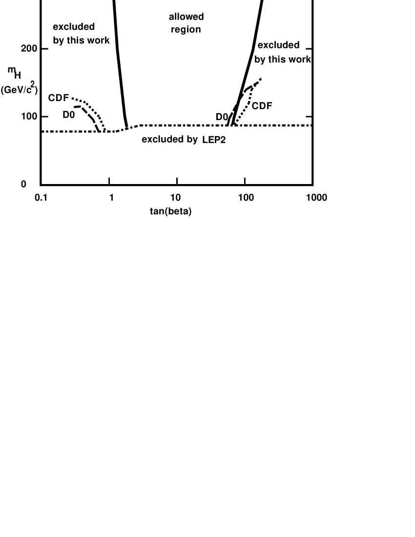
Figure 2.2: Lower and upper limits on $\tan\beta$ as a function of the mass of the charged Higgs $m_{H}$ from meson decay, mixing and CP violation (continuous curve) compared to limits obtained by CDF[18], D0[19] and LEP2[20], all at $95\%$ confidence.

2.5 Conclusions

Using measured meson decay rates, mixing and CP violation we have obtained lower and upper bounds of $\tan\beta$ for each $m_{H}$. These limits are compared with the results of direct searches in Figures 2.2. Note that the measurements of $\sin(2\beta_{CKM})$ by the Belle and BaBar collaborations have raised the lower bound on $\tan\beta$ by a factor $\approx 5$ with respect to our previous calculation [4]. It is important to mention that an indirect limit by the CLEO collaboration [21] obtained from the measurements of the $b\rightarrow s\gamma$ transition, limits the Two Higgs Doublet Model of type II to have a charged Higgs mass in excess of about $264\textrm{GeV/c}^{2}$ (it is a slow function of $\tan\beta$).

Chapter 3 Mass constraints, production cross sections, and decay rates in the Two Higgs Doublet Model of type II

3.1 Introduction

Among the extensions of the Standard Model that respect its principles and symmetries, and are compatible with present data within a region of parameter space, and are of interest at the large particle colliders, is the addition of a second doublet of Higgs fields. In this article we consider the Two Higgs Doublet Model of type II[1]. The Higgs sector of the Minimal Supersymmetric Standard Model (MSSM) is of this type (tho the model of type II does not require Supersymmetry). The physical spectrum of the model contains five Higgs bosons: one pseudoscalar $A^{o}$ (CP-odd scalar), two neutral scalars $H^{o}$ and $h^{o}$ (CP-even scalars), and two charged scalars $H^{+}$ and $H^{-}$. The masses of the charged Higgs bosons $m_{H}$, and the ratio of the vacuum expectation values of the two neutral components of the Higgs doublets, $\tan\beta>0$, are free parameters of the theory.

In [2] we obtained limits in the $(m_{H},\tan\beta)$ plane using measured decay rates, mixing and CP violation of mesons. In this article we present graphically the corresponding limits on $m_{H^{0}}$, $m_{h^{0}}$ and $m_{A^{0}}$. Then we calculate production cross sections, decay rates and branching fractions of the Higgs particles. Next, we obtain the running coupling constants and discuss Grand Unification. Finally, in the Conclusions, we list interesting discovery channels.

3.2 Masses

The masses of the neutral Higgs particles as a function of the masses of the charged Higgs $m_{H}$, $\tan\beta$ and the masses of $Z$ and $W$, calculated at tree level, are:

$$m_{A^{0}}^{2}=m_{H}^{2}-m_{W}^{2},$$ (3.1)

$$2m_{H^{0}}^{2}=m_{H}^{2}-m_{W}^{2}+m_{Z}^{2}$$ (3.2)

$$+\left[\left(m_{H}^{2}-m_{W}^{2}+m_{Z}^{2}\right)^{2}-4m_{Z}^{2}\left(m_{H}^{2}-m_{W}^{2}\right)\left(\frac{\tan^{2}\beta-1}{\tan^{2}\beta+1}\right)^{2}\right]^{\frac{1}{2}}$$

$$2m_{h^{0}}^{2}=m_{H}^{2}-m_{W}^{2}+m_{Z}^{2}$$ (3.3)

$$-\left[\left(m_{H}^{2}-m_{W}^{2}+m_{Z}^{2}\right)^{2}-4m_{Z}^{2}\left(m_{H}^{2}-m_{W}^{2}\right)\left(\frac{\tan^{2}\beta-1}{\tan^{2}\beta+1}\right)^{2}\right]^{\frac{1}{2}}$$

We have re derived these equations in agreement with the literature.[1]

In Chapter two [2] we obtained the limits in the $(\tan\beta,m_{H})$ plane shown in Figure 3.1. From that figure and Equations 3.1, 3.2 and 3.3 we obtain the limits on the masses of the neutral Higgs particles shown in Figure 3.2.

Radiative corrections can be very large. In the MSSM the largest contributions arise from the incomplete cancellation between top and stop loops. The corresponding plot similar to Figure 3.2 with radiative corrections can be found in [6].

Figure 3.1: Lower and upper limits on $\tan\beta$ as a function of the mass of the charged Higgs $m_{H}$ from meson decay, mixing and CP violation (continuous curve) compared to limits obtained by CDF[3], D0[4] and LEP2[5], all at $95\%$ confidence. Taken from [2].

Figure 3.2: Allowed regions of the masses of the neutral Higgs $h^{0}$, $H^{0}$ and $A^{0}$ as a function of the mass $m_{H}$ of the charged Higgs $H^{\pm}$. From Figure 3.1 and the tree level Equations 3.1, 3.2 and 3.3. Radiative corrections raise the allowed region of $h^{0}$.[6]

3.3 Feynman rules

The Lagrangian for the $VHH$ interaction is:[1]

$$\mathcal{L}_{VHH} = \frac{-ig}{2}W_{\mu}^{+}\cdot H^{-}\overleftrightarrow{\partial}^{\mu}\left[H^{0}\sin(\alpha-\beta)+h^{0}\cos(\alpha-\beta)+iA^{0}\right]+\mathrm{h.c.}$$ (3.4)

$$-\frac{ig}{2\cos\theta_{W}}Z_{\mu}\{iA^{0}\overleftrightarrow{\partial}^{\mu}\left[H^{0}\sin(\alpha-\beta)+h^{0}\cos(\alpha-\beta)\right]$$

$$-\left(2\sin^{2}\theta_{W}-1\right)\cdot H^{-}\overleftrightarrow{\partial}^{\mu}H^{+}\}$$

where

$$A\overleftrightarrow{\partial}^{\mu}B=A(\partial^{\mu}B)-(\partial^{\mu}A)B.$$ (3.5)

The Lagrangian for the $VVH$ interaction is:

$$\mathcal{L}_{VVH} = \left(gm_{W}W_{\mu}^{+}W^{-\mu}+\frac{gm_{Z}}{2\cos\theta_{W}}Z_{\mu}Z^{\mu}\right)$$ (3.6)

$$\times\left[H^{0}\cos(\beta-\alpha)+h^{0}\sin(\beta-\alpha)\right].$$

There are no vertices $ZH^{0}H^{0}$, $Zh^{0}h^{0}$, $ZA^{0}A^{0}$, $ZW^{+}H^{-}$ or $ZH^{0}h^{0}$. The interactions of neutral Higgs bosons with up and down quarks are given by:

$$\mathcal{L}_{AHhff^{\prime}} = \frac{-gm_{f}}{2m_{W}\sin\beta}\left[\bar{u}_{f}v_{\bar{f}}(H^{0}\sin\alpha+h^{0}\cos\alpha)-i\cos\beta\cdot\bar{u}_{f}\gamma^{5}v_{\bar{f}}A^{0}\right]$$ (3.7)

$$-\frac{gm_{f^{\prime}}}{2m_{W}\cos\beta}$$

$$\times\left[\bar{u}_{f^{\prime}}v_{\bar{f^{\prime}}}(H^{0}\cos\alpha-h^{0}\sin\alpha)-i\sin\beta\cdot\bar{u}_{f^{\prime}}\gamma^{5}v_{\bar{f^{\prime}}}A^{0}\right]$$

where $f=u,c,t,\nu_{e},\nu_{\mu},\nu_{\tau}$ and $f^{\prime}=d,s,b,e^{-},\mu^{-},\tau^{-}$. The Lagrangian corresponding to the $H^{\pm}f\bar{f}^{\prime}$ vertex is:

$$\mathcal{L}_{H^{\pm}ff^{\prime}} = \frac{g}{2\sqrt{2}m_{W}}\{H^{+}V_{ff^{\prime}}\bar{u}_{f}\left(A+B\gamma^{5}\right)v_{\bar{f}^{\prime}}$$ (3.8)

$$+H^{-}V_{ff^{\prime}}^{*}\bar{u}_{f^{\prime}}(A-B\gamma^{5})v_{\bar{f}}\}$$

where $A\equiv\left(m_{f^{\prime}}\tan\beta+m_{f}\cot\beta\right)$ and $B\equiv\left(m_{f^{\prime}}\tan\beta-m_{f}\cot\beta\right)$. $V_{ff^{\prime}}$ is an element of the CKM matrix. The Lagrangian corresponding to three Higgs bosons is:

$$\mathcal{L}_{3h} = -gH^{0}\{H^{+}H^{-}\left[m_{W}\cos(\beta-\alpha)-\frac{m_{Z}}{2\cos\theta_{W}}\cos(2\beta)\cos(\beta+\alpha)\right]$$ (3.9)

$$+\frac{m_{Z}}{4\cos\theta_{W}}H^{0}H^{0}\cos(2\alpha)\cos(\beta+\alpha)$$

$$+\frac{m_{Z}}{4\cos\theta_{W}}h^{0}h^{0}\left[2\sin(2\alpha)\sin(\beta+\alpha)-\cos(\beta+\alpha)\cos(2\alpha)\right]$$

$$-\frac{m_{Z}}{4\cos\theta_{W}}A^{0}A^{0}\cos(2\beta)\cos(\beta+\alpha)\}$$

$$-gh^{0}\{H^{+}H^{-}\left[m_{W}\sin(\beta-\alpha)+\frac{m_{Z}}{2\cos\theta_{W}}\cos(2\beta)\sin(\beta+\alpha)\right]$$

$$+\frac{m_{Z}}{4\cos\theta_{W}}h^{0}h^{0}\cos(2\alpha)\sin(\beta+\alpha)$$

$$-\frac{m_{Z}}{4\cos\theta_{W}}H^{0}H^{0}\left[2\sin(2\alpha)\cos(\beta+\alpha)+\sin(\beta+\alpha)\cos(2\alpha)\right]$$

$$+\frac{m_{Z}}{4\cos\theta_{W}}A^{0}A^{0}\cos(2\beta)\sin(\beta+\alpha)\}.$$

Vertexes with four partons including two Higgs bosons are

$$\mathcal{L}_{4} = e^{2}A_{\mu}A^{\mu}H^{+}H^{-}+\frac{eg\cos\left(2\theta_{W}\right)}{\cos\theta_{W}}A_{\mu}Z^{\mu}H^{+}H^{-}$$ (3.10)

$$-\frac{eg}{2}\sin\left(\beta-\alpha\right)A_{\mu}W^{\pm\mu}H^{0}H^{\mp}+\frac{eg}{2}\cos\left(\beta-\alpha\right)A_{\mu}W^{\pm\mu}h^{0}H^{\mp}$$

$$\pm\frac{ige}{2}A_{\mu}W^{\pm\mu}A^{0}H^{\mp},$$

The $H^{+}H^{-}\gamma$ vertex is

$$\mathcal{L}_{H^{+}H^{-}\gamma}=-ig\sin\theta_{W}A_{\mu}H^{-}\overleftrightarrow{\partial^{\mu}}H^{+}$$ (3.11)

The Higgs propagators are: $i/\left(k^{2}-m^{2}+i\varepsilon\right)$.

Feynman diagrams corresponding to the production of $Zh^{0}$ are shown in Figures 3.3, 3.4 and 3.5. Note that the invariant mass of $Zh^{0}$ can have a resonance at $m_{A^{0}}$ which is an interesting experimental signature. Feynman diagrams corresponding to the production of $W^{\pm}h^{0}$ or $W^{\pm}H^{0}$ are shown in Figure 3.6.

Figure 3.3: Feynman diagrams corresponding to the production of $h^{0}$ in the
channel $q\bar{q}\rightarrow h^{0}Z^{0}$.

Figure 3.4: Feynman diagrams corresponding to the production of $h^{0}$ in the
channel $gg\rightarrow h^{0}Z^{0}$. Continued in Figure 3.5.

Figure 3.5: Continued from Figure 3.4.

Figure 3.6: Feynman diagrams corresponding to the production of $h^{0}W^{\pm}$ and $H^{0}W^{\pm}$.

3.4 Decay rates of $h^{0}$

Calculating the Feynman diagrams of Figure 3.7 we obtain the decay rate corresponding to $h^{0}\rightarrow gg$:

$$\Gamma(h^{0}\rightarrow gg) = \frac{\sqrt{2}G_{F}\alpha_{s}^{2}m_{h^{0}}^{3}}{64\pi^{3}}\frac{\cos^{2}{\alpha}}{\sin^{2}\beta}|\tan\beta\tan\alpha\tau_{b}\left[\left(\tau_{b}-1\right)f(\tau_{b})+2\right]$$ (3.12)

$$-\tau_{t}\left[\left(\tau_{t}-1\right)f(\tau_{t})+2\right]|^{2}$$

where

$$\tau_{i}=\frac{4m_{i}^{2}}{m_{h^{0}}^{2}},$$ (3.13)

(note that $\tau_{i}$ will change from Section to Section),

$$f(\tau_{i})=\left\{\begin{array}[]{ll}-2\left[\arcsin\left(\tau_{i}^{-1/2}\right)\right]^{2}&\mbox{if $\tau_{i}>1$}\\ \frac{1}{2}\left[\ln\left(\frac{1+\left(1-\tau_{i}\right)^{1/2}}{1-\left(1-\tau_{i}\right)^{1/2}}\right)-i\pi\right]^{2}&\mbox{if $\tau_{i}\leq 1$,}\end{array}\right.$$ (3.14)

$$\tan\alpha=-\left\{\frac{1+F}{1-F}\right\}^{\frac{1}{2}},$$ (3.15)

$$F=\frac{1-\tan^{2}\beta}{\left(1+\tan^{2}\beta\right)G}\left[1-\frac{m_{Z}^{2}}{m_{H}^{2}}-\frac{m_{W}^{2}}{m_{H}^{2}}\right],$$ (3.16)

$$G=\left[\left(1+\frac{m_{Z}^{2}}{m_{H}^{2}}-\frac{m_{W}^{2}}{m_{H}^{2}}\right)^{2}-4\frac{m_{Z}^{2}}{m_{H}^{2}}\left(1-\frac{m_{W}^{2}}{m_{H}^{2}}\right)\left(\frac{\tan^{2}\beta-1}{\tan^{2}\beta+1}\right)^{2}\right]^{\frac{1}{2}}.$$ (3.17)

Calculating the Feynman diagrams of Figure 3.8 we obtain:

$$\Gamma\left(h^{0}\rightarrow c\bar{c}\right)=\frac{3G_{F}m_{c}^{2}m_{h^{0}}\cos^{2}\alpha}{\sqrt{2}\cdot 4\pi\sin^{2}\beta}\left(1-\frac{4m_{c}^{2}}{m_{h^{0}}^{2}}\right)^{\frac{3}{2}},$$ (3.18)

$$\Gamma\left(h^{0}\rightarrow b\bar{b}\right)=\frac{3G_{F}m_{b}^{2}m_{h^{0}}\sin^{2}\alpha}{\sqrt{2}\cdot 4\pi\cos^{2}\beta}\left(1-\frac{4m_{b}^{2}}{m_{h^{0}}^{2}}\right)^{\frac{3}{2}},$$ (3.19)

and

$$\Gamma\left(h^{0}\rightarrow\tau^{-}\tau^{+}\right)=\frac{G_{F}m_{\tau}^{2}m_{h^{0}}\sin^{2}\alpha}{\sqrt{2}\cdot 4\pi\cos^{2}\beta}\left(1-\frac{4m_{\tau}^{2}}{m_{h^{0}}^{2}}\right)^{\frac{3}{2}}.$$ (3.20)

Figure 3.7: Feynman diagrams corresponding to the decay $h^{0}\rightarrow gg$.

Figure 3.8: Feynman diagram corresponding to the decays $h^{0}\rightarrow b\bar{b},c\bar{c},\tau\bar{\tau}$.

3.5 Branching fractions of $h^{0}$

From the preceding decay rates we obtain the following branching fractions for the case $m_{b},m_{c},m_{\tau}\ll m_{h^{0}}<120$GeV/c²:

$$B\left(h^{0}\rightarrow b\bar{b}\right)=\frac{3m_{b}^{2}\sin^{2}\alpha}{3m_{b}^{2}\sin^{2}\alpha+3m_{c}^{2}\cos^{2}\alpha\cot^{2}\beta+m_{\tau}^{2}\sin^{2}\alpha+J}$$ (3.21)

and

$$B\left(h^{0}\rightarrow\tau^{+}\tau^{-}\right)=\frac{m_{\tau}^{2}\sin^{2}\alpha}{3m_{b}^{2}\sin^{2}\alpha+3m_{c}^{2}\cos^{2}\alpha\cot^{2}\beta+m_{\tau}^{2}\sin^{2}\alpha+J}$$ (3.22)

where

$$J = \frac{\alpha_{s}^{2}m_{h^{0}}^{2}}{8\pi^{2}}\frac{\cos^{2}\alpha}{\tan^{2}\beta}|\tan\beta\tan\alpha\left[\tau_{b}\left(-\frac{1}{2}\left\{\ln\left(\frac{\tau_{b}}{4}\right)+i\pi\right\}^{2}+2\right)\right]$$ (3.23)

$$-\tau_{t}\left\{\left(\tau_{t}-1\right)f\left(\tau_{t}\right)+2\right\}|^{2}.$$

For $90<m_{H}<1000$GeV/c², $B\left(h^{0}\rightarrow b\bar{b}\right)$ varies from 0.856 to 0.944. Neglecting $B\left(h^{0}\rightarrow gg\right)$ and the contribution of $c\bar{c}$ we obtain

$$B\left(h^{0}\rightarrow b\bar{b}\right)=\frac{3m_{b}^{2}}{3m_{b}^{2}+m_{\tau}^{2}}=0.944$$ (3.24)

and

$$B\left(h^{0}\rightarrow\tau^{+}\tau^{-}\right)=\frac{m_{\tau}^{2}}{3m_{b}^{2}+m_{\tau}^{2}}=0.056.$$ (3.25)

3.6 Decay rates of $H^{\pm}$

The tree level Feynman diagram of Figure 3.9 gives the following decay rate:

$$\Gamma\left(H^{\pm}\rightarrow W^{\pm}h^{0}\right) = \frac{\sqrt{2}G_{F}\cos^{2}{\alpha}}{16\pi m_{H}^{3}\left(1+\tan^{2}{\beta}\right)}\left[1+\tan{\beta}\tan{\alpha}\right]^{2}$$ (3.26)

$$\times\Lambda^{3/2}\left(m_{H}^{2},m_{W}^{2},m_{h^{0}}^{2}\right)$$

where

$$\Lambda(a,b,c)=a^{2}+b^{2}+c^{2}-2ab-2bc-2ca.$$ (3.27)

Similarly from the Feynman diagrams of Figures 3.10 and 3.11 we obtain

$$\Gamma\left(H^{\pm}\rightarrow W^{\pm}H^{0}\right) = \frac{\sqrt{2}G_{F}\left(\tan\beta-\tan\alpha\right)^{2}}{16\pi m_{H}^{3}\left(1+\tan^{2}{\beta}\right)\left(1+\tan^{2}{\alpha}\right)}$$ (3.28)

$$\times\Lambda^{3/2}\left(m_{H}^{2},m_{W}^{2},m_{H^{0}}^{2}\right),$$

$$\Gamma\left(H^{\pm}\rightarrow W^{\pm}A^{0}\right)=\frac{\sqrt{2}G_{F}}{16\pi m_{H}^{3}}\Lambda^{3/2}\left(m_{A^{0}}^{2},m_{W}^{2},m_{H}^{2}\right).$$ (3.29)

Figure 3.9: Feynman diagram corresponding to the decay $H^{\pm}\rightarrow W^{\pm}h^{0}$.

Figure 3.10: Feynman diagram corresponding to the decay $H^{\pm}\rightarrow W^{\pm}H^{0}$.

Figure 3.11: Feynman diagram corresponding to the decay $H^{\pm}\rightarrow W^{\pm}A^{0}$.

3.7 Decays of $H^{0}$.

The tree level Feynman diagrams of Figure 3.12 give the following decay rates:

$$\Gamma(H^{0}\rightarrow f\bar{f})=\frac{\sqrt{2}G_{F}m_{f}^{2}m_{H^{0}}}{8\pi}\left(1-\frac{4m_{f}^{2}}{m_{H^{0}}^{2}}\right)^{3/2}N_{f}B_{f}^{2}$$ (3.30)

where $N_{f}=3$ for quarks, $N_{f}=1$ for leptons, $B_{f}^{2}=\sin^{2}\alpha(1+\cot^{2}\beta)$ for $f=u,c,t$, and $B_{f}^{2}=\cos^{2}\alpha(1+\tan^{2}\beta)$ for $f=d,s,b,e^{-},\mu^{-},\tau^{-}$.

From the Feynman diagrams of Figure 3.13 we obtain

$$\Gamma(H^{0}\rightarrow gg) = \frac{\sqrt{2}G_{F}\alpha_{s}^{2}m_{H^{0}}^{3}}{64\pi^{3}}\sin^{2}\alpha(1+\cot^{2}\beta)$$ (3.31)

$$\times|\frac{\tan\beta}{\tan\alpha}\tau_{b}\left[(\tau_{b}-1)f(\tau_{b})+2\right]$$

$$+{\tau_{t}\left[(\tau_{t}-1)f(\tau_{t})+2\right]}|^{2}$$

where

$$\tau_{i}=\frac{4m_{i}^{2}}{m_{H^{0}}^{2}}.$$ (3.32)

From the Feynman diagram of Figure 3.14 we obtain

$$\Gamma\left(H^{0}\rightarrow h^{0}h^{0}\right)=\frac{\sqrt{2}G_{F}m_{Z}^{4}}{32\pi m_{H^{0}}}$$ (3.33)

$$\times\left(1-\frac{4m_{h^{0}}^{2}}{m_{H^{0}}^{2}}\right)^{1/2}\frac{\left(1-\tan^{2}\alpha\right)^{2}}{\left(1+\tan^{2}\alpha\right)^{3}\left(1+\tan^{2}\beta\right)}$$

$$\times\left[\frac{4\tan\alpha}{1-\tan^{2}\alpha}\left(\tan\alpha+\tan\beta\right)-\left(1-\tan\alpha\tan\beta\right)\right]^{2}.$$

From the Feynman diagrams of Figures 3.15 and 3.16 we obtain

$$\Gamma\left(H^{0}\rightarrow A^{0}A^{0}\right)=\frac{\sqrt{2}G_{F}m_{Z}^{4}}{32\pi m_{H^{0}}}\left(1-\frac{4m_{A^{0}}^{2}}{m_{H^{0}}^{2}}\right)^{1/2}$$ (3.34)

$$\times\frac{\left(\tan^{2}\beta-1\right)^{2}}{\left(1+\tan^{2}\alpha\right)\left(1+\tan^{2}\beta\right)^{3}}\left[1-\tan\alpha\tan\beta\right]^{2},$$

$$\Gamma\left(H^{0}\rightarrow ZZ\right) = \frac{\sqrt{2}G_{F}\left(1+\tan\beta\tan\alpha\right)^{2}m_{H^{0}}^{3}}{32\pi\left(1+\tan^{2}\beta\right)\left(1+\tan^{2}\alpha\right)}$$ (3.35)

$$\times\left(12x^{2}-4x+1\right)\left(1-4x\right)^{1/2}$$

where

$$x=\frac{m_{Z}^{2}}{m_{H^{0}}^{2}}.$$ (3.36)

Similarly, from the diagram of Figure 3.17 we obtain

$$\Gamma\left(H^{0}\rightarrow W^{+}W^{-}\right) = \frac{\sqrt{2}G_{F}\left(1+\tan\beta\tan\alpha\right)^{2}m_{H^{0}}^{3}}{16\pi\left(1+\tan^{2}\beta\right)\left(1+\tan^{2}\alpha\right)}$$ (3.37)

$$\times\left(12y^{2}-4y+1\right)\left(1-4y\right)^{1/2}$$

where

$$y=\frac{m_{W}^{2}}{m_{H^{0}}^{2}}.$$ (3.38)

From the Feynman diagram of Figure 3.18 we obtain

$$\Gamma\left(H^{0}\rightarrow W^{\pm}H^{\mp}\right) = \frac{\sqrt{2}G_{F}\left(\tan\alpha-\tan\beta\right)^{2}}{16\pi m_{H^{0}}^{3}\left(1+\tan^{2}\alpha\right)\left(1+\tan^{2}\beta\right)}$$ (3.39)

$$\times\Lambda^{3/2}\left(m_{H^{0}}^{2},m_{W}^{2},m_{H}^{2}\right).$$

From the Feynman diagram of Figure 3.19 we obtain

$$\Gamma\left(H^{0}\rightarrow H^{+}H^{-}\right)=\frac{\sqrt{2}G_{F}m_{W}^{4}}{4\pi m_{H^{0}}\left(1+\tan^{2}\beta\right)\left(1+\tan^{2}\alpha\right)}$$ (3.40)

$$\times\left[\left(1+\tan\beta\tan\alpha\right)-\frac{\left(1-\tan\beta\tan\alpha\right)}{2\cos^{2}\theta_{W}}\frac{1-\tan^{2}\beta}{1+\tan^{2}\beta}\right]^{2}$$

$$\times\left(1-\frac{4m_{H}^{2}}{m_{H^{0}}^{2}}\right)^{1/2}.$$

The Feynman diagrams corresponding to $h^{0},H^{0}\rightarrow\gamma\gamma$ are shown in Figure 3.20.

$$\Gamma(H^{0}\rightarrow h^{0}Z)=0.$$ (3.41)

Figure 3.12: Feynman diagram corresponding to the decay $H^{0}\rightarrow f\bar{f}$.

Figure 3.13: Feynman diagrams corresponding to the decay $H^{0}\rightarrow gg$.

Figure 3.14: Feynman diagram corresponding to the decay $H^{0}\rightarrow h^{0}h^{0}$.

Figure 3.15: Feynman diagram corresponding to the decay $H^{0}\rightarrow A^{0}A^{0}$.

Figure 3.16: Feynman diagram corresponding to the decay $H^{0}\rightarrow ZZ$.

Figure 3.17: Feynman diagram corresponding to the decay $H^{0}\rightarrow W^{+}W^{-}$.

Figure 3.18: Feynman diagram corresponding to the decay $H^{0}\rightarrow W^{\pm}H^{\mp}$.

Figure 3.19: Feynman diagram corresponding to the decay $H^{0}\rightarrow H^{+}H^{-}$.

Figure 3.20: Feynman diagrams corresponding to $h^{0},H^{0}\rightarrow\gamma\gamma$.

3.8 Decay rates of $A^{0}$

From the tree level Feynman diagram of Figure 3.21 we obtain

$$\Gamma\left(A^{0}\rightarrow Zh^{0}\right)=\frac{\sqrt{2}G_{F}\cos^{2}{\alpha}}{16\pi m_{A^{0}}^{3}\left(1+\tan^{2}{\beta}\right)}$$ (3.42)

$$\times\left[1+\tan{\beta}\tan{\alpha}\right]^{2}\Lambda^{3/2}\left(m_{A^{0}}^{2},m_{h^{0}}^{2},m_{Z}^{2}\right)$$

From the tree level diagram of Figure 3.22 we obtain

$$\Gamma\left(A^{0}\rightarrow f\bar{f}\right)=\frac{\sqrt{2}G_{F}}{8\pi}m_{A^{0}}m_{f}^{2}A_{f}^{2}\left(1-\frac{4m_{f}^{2}}{m_{A^{0}}^{2}}\right)^{1/2}N_{f}$$ (3.43)

where $N_{f}=3$ for quarks, $N_{f}=1$ for leptons, $A_{f}=\cot{\beta}$ for $f=u,c,t$,

and $A_{f}=\tan{\beta}$ for $f=d,s,b,e^{-},\mu^{-},\tau^{-}$.

From the Feynman diagrams shown in Figure 3.23 we obtain (see Appendix D):

$$\Gamma\left(A^{0}\rightarrow Z\gamma\right)=\frac{\sqrt{2}G_{F}\alpha_{em}^{2}m_{A^{0}}^{3}}{512\pi^{3}\sin^{2}{\theta_{W}}\cos^{2}{\theta_{W}}}\left(1-\frac{m_{Z}^{2}}{m_{A^{0}}^{2}}\right)^{3}$$ (3.44)

$$\times|\tan{\beta}\{\left(\frac{1}{2}-\frac{2}{3}\sin^{2}{\theta_{W}}\right)I\left(\tau_{b},\Lambda_{b}\right)$$

$$+\left(\frac{1}{2}-2\sin^{2}{\theta_{W}}\right)I\left(\tau_{\tau},\Lambda_{\tau}\right)\}$$

$$+2\cot{\beta}\left(\frac{1}{2}-\frac{4}{3}\sin^{2}{\theta_{W}}\right)I\left(\tau_{t},\Lambda_{t}\right)|^{2}$$

where

$$\tau_{i}=\frac{4m_{i}^{2}}{m_{A^{0}}^{2}},\qquad\Lambda_{i}=\frac{4m_{i}^{2}}{m_{Z}^{2}},$$ (3.45)

and

$$I\left(\tau_{i},\Lambda_{i}\right)=\frac{\tau_{i}\Lambda_{i}}{\Lambda_{i}-\tau_{i}}\left\{f(\tau_{i})-f(\Lambda_{i})\right\}.$$ (3.46)

From the Feynman diagrams of Figure 3.24 we obtain the decay rate:

$$\Gamma(A^{0}\rightarrow gg)=\frac{\sqrt{2}G_{F}\alpha_{s}^{2}m_{A^{0}}^{3}}{128\pi^{3}}|\tan\beta\tau_{b}f(\tau_{b})+\cot\beta\tau_{t}f(\tau_{t})|^{2}.$$ (3.47)

$$\Gamma\left(A^{0}\rightarrow h^{0}h^{0}\right)=\Gamma\left(A^{0}\rightarrow H^{0}H^{0}\right)=0.$$ (3.48)

From the Feynman diagram 3.25 we obtain

$$\Gamma\left(A^{0}\rightarrow W^{\pm}H^{\mp}\right)=\frac{\sqrt{2}G_{F}}{16\pi m_{A^{0}}^{3}}\Lambda^{3/2}\left(m_{A^{0}}^{2},m_{W}^{2},m_{H}^{2}\right).$$ (3.49)

From the Feynman diagram 3.26 we obtain

$$\Gamma\left(A^{0}\rightarrow ZH^{0}\right) = \frac{\sqrt{2}G_{F}\left(\tan\beta-\tan\alpha\right)^{2}}{16\pi m_{A^{0}}^{3}\left(1+\tan^{2}\alpha\right)\left(1+\tan^{2}\beta\right)}$$ (3.50)

$$\times\Lambda^{3/2}\left(m_{A^{0}}^{2},m_{H^{0}}^{2},m_{Z}^{2}\right).$$

From the Feynman diagrams of 3.27 we obtain:

$$\Gamma\left(A^{0}\rightarrow\gamma\gamma\right) = \frac{\sqrt{2}G_{F}\alpha^{2}_{em}m^{3}_{A^{0}}}{256\pi^{3}}\left|\tan\beta\left[\frac{1}{3}\tau_{b}f(\tau_{b})+\tau_{\tau}f(\tau_{\tau})\right]\right.$$ (3.51)

$$\left.+\cot\beta\left[\frac{4}{3}\tau_{t}f(\tau_{t})\right]\right|^{2}$$

Figure 3.21: Feynman diagram corresponding to the decay $A^{0}\rightarrow Zh^{0}$.

Figure 3.22: Feynman diagram corresponding to the decay $A^{0}\rightarrow f\bar{f}$.

Figure 3.23: Feynman diagrams corresponding to the decay $A^{0}\rightarrow Z\gamma$.

Figure 3.24: Feynman diagrams of $A^{0}\rightarrow gg$.

Figure 3.25: Feynman diagram of $A^{0}\rightarrow W^{\pm}H^{\mp}$.

Figure 3.26: Feynman diagram of $A^{0}\rightarrow ZH^{0}$.

Figure 3.27: Feynman diagrams for $A^{0}\rightarrow\gamma\gamma$.

3.9 Decay $Z\rightarrow h^{0}\gamma$

From the Feynman diagrams of Figure 3.28 we obtain:

$$\Gamma\left(Z\rightarrow h^{0}\gamma\right) = \frac{\sqrt{2}G_{F}\alpha_{em}^{2}m_{Z}^{3}}{64\pi^{3}\sin^{2}{\theta_{W}}\cos^{2}{\theta_{W}}}\left(1-\frac{m_{h^{0}}^{2}}{m_{Z}^{2}}\right)^{3}\cos^{2}\alpha\cos^{2}\beta$$ (3.52)

$$\times\mathopen{|}\frac{1}{\cos\beta\sin\beta}[\tan{\alpha}\tan{\beta}\left(\frac{1}{2}-\frac{2}{3}\sin^{2}{\theta_{W}}\right)F(\tau_{b},\Lambda_{b})$$

$$+\tan{\alpha}\tan{\beta}\left(\frac{1}{2}-2\sin^{2}{\theta_{W}}\right)F(\tau_{\tau},\Lambda_{\tau})$$

$$-2\left(\frac{1}{2}-\frac{4}{3}\sin^{2}{\theta_{W}}\right)F(\tau_{t},\Lambda_{t})]$$

$$+\left[\tan\beta-\tan\alpha+\frac{1-\tan^{2}\beta}{1+\tan^{2}\beta}\frac{\tan\beta+\tan\alpha}{2\cos^{2}\theta_{W}}\right]$$

$$\times\frac{m_{W}^{2}}{2m_{H}^{2}}(1-2\sin^{2}\theta_{W})I(\tau_{H},\Lambda_{H})$$

$$-\frac{1}{2}\left(\tan\beta-\tan\alpha\right)\cos^{2}\theta_{W}[4\left(3-\tan^{2}\theta_{W}\right)K(\tau_{W},\Lambda_{W})$$

$$+\left\{\left(1+\frac{2}{\tau_{W}}\right)\tan^{2}\theta_{W}-\left(5+\frac{2}{\tau_{W}}\right)\right\}$$

$$\times I(\tau_{W},\Lambda_{W})]\mathclose{|}^{2}$$

where

$$\tau_{i}=\frac{4m_{i}^{2}}{m_{h^{0}}^{2}},\qquad\Lambda_{i}=\frac{4m_{i}^{2}}{m_{Z}^{2}},\qquad\tau_{H}=\frac{4m_{H}^{2}}{m_{h^{0}}^{2}},\qquad\Lambda_{H}=\frac{4m_{H}^{2}}{m_{Z}^{2}},$$ (3.53)

$$F(\tau_{i},\Lambda_{i}) = -\frac{1}{2}\frac{\tau_{i}\Lambda_{i}}{\tau_{i}-\Lambda_{i}}-\frac{\tau_{i}^{2}\Lambda_{i}}{\left(\tau_{i}-\Lambda_{i}\right)^{2}}\left\{g(\tau_{i})-g(\Lambda_{i})\right\}$$ (3.54)

$$+\frac{1}{4}\frac{\tau_{i}\Lambda_{i}}{\tau_{i}-\Lambda_{i}}\left[1+\frac{\tau_{i}\Lambda_{i}}{\tau_{i}-\Lambda_{i}}\right]\left\{f(\tau_{i})-f(\Lambda_{i})\right\},$$

$$g(x)=\left\{\begin{array}[]{ll}\left(x-1\right)^{1/2}\arcsin{\left(x^{-1/2}\right)}&\mbox{if $x\geq 1$}\\ \frac{1}{2}\left(1-x\right)^{1/2}\left[\ln{\left\{\frac{1+(1-x)^{1/2}}{1-(1-x)^{1/2}}\right\}}-i\pi\right]&\mbox{if $x<1$,}\end{array}\right.$$ (3.55)

$$I(\tau_{H},\Lambda_{H}) = -\frac{1}{2}\frac{\tau_{H}\Lambda_{H}}{(\tau_{H}-\Lambda_{H})}-\frac{\tau_{H}^{2}\Lambda_{H}}{(\tau_{H}-\Lambda_{H})^{2}}\left[g(\tau_{H})-g(\Lambda_{H})\right]$$ (3.56)

$$+\frac{1}{4}\frac{\tau_{H}^{2}\Lambda_{H}^{2}}{(\tau_{H}-\Lambda_{H})^{2}}\left[f(\tau_{H})-f(\Lambda_{H})\right],$$

$$\tau_{W}=\frac{4m_{W}^{2}}{m_{h^{0}}^{2}},\qquad\Lambda_{W}=\frac{4m_{W}^{2}}{m_{Z}^{2}},$$ (3.57)

$$K(\tau_{W},\Lambda_{W})=-\frac{\tau_{W}\Lambda_{W}}{4(\tau_{W}-\Lambda_{W})}[f(\tau_{W})-f(\Lambda_{W})].$$ (3.58)

The decay width of Equation 3.52 turns out to be negligible compared to the full width of $Z$ so we can not use it to constrain the mass of $h^{0}$.

Figure 3.28: Feynman diagrams for $Z\rightarrow h^{0}\gamma$.

3.10 Vertex with four particles

The decay rate corresponding to the Feynman diagram 3.29 is:

$$\Gamma\left(H^{\pm}\rightarrow W^{\pm}\gamma h^{0}\right)=\frac{3G_{F}^{2}\sin^{2}\theta_{W}\left(1+\tan\beta\tan\alpha\right)^{2}m_{W}^{5}}{32\left(1+\tan^{2}\beta\right)\left(1+\tan^{2}\alpha\right)\pi^{3}\left(x_{H}^{W}\right)^{1/2}}$$ (3.59)

$$\times\{\frac{1}{2}\Lambda^{\frac{1}{2}}\left(1,x_{H}^{W},x_{H}^{h^{0}}\right)\left(1+x_{H}^{W}+x_{H}^{h^{0}}\right)$$

$$+\left(2x_{H}^{W}x_{H}^{h^{0}}-x_{H}^{W}-x_{H}^{h^{0}}\right)\times\ln\left|\frac{\Lambda^{\frac{1}{2}}\left(1,x_{H}^{W},x_{H}^{h^{0}}\right)+1-x_{H}^{W}-x_{H}^{h^{0}}}{2\left(x_{H}^{W}x_{H}^{h^{0}}\right)^{1/2}}\right|$$

$$-\left|x_{H}^{h^{0}}-x_{H}^{W}\right|\times$$

$$\ln\left|\frac{\left|x_{H}^{h^{0}}-x_{H}^{W}\right|\Lambda^{\frac{1}{2}}\left(1,x_{H}^{W},x_{H}^{h^{0}}\right)-\left(x_{H}^{W}+x_{H}^{h^{0}}\right)+\left(x_{H}^{W}-x_{H}^{h^{0}}\right)^{2}}{2\left(x_{H}^{W}x_{H}^{h^{0}}\right)^{1/2}}\right|\}$$

where

$$x_{H}^{W}=\frac{m_{W}^{2}}{m_{H}^{2}},\qquad x_{H}^{h^{0}}=\frac{m_{h^{0}}^{2}}{m_{H}^{2}}.$$ (3.60)

Figure 3.29: Diagram for $H^{\pm}\rightarrow W^{\pm}\gamma h^{0}$.

Figure 3.30: Feynman diagrams for $p\bar{p}\rightarrow AX$ with $A\equiv h^{0},H^{0},A^{0}$.

3.11 Production of $h^{0}$, $H^{0}$ and $A^{0}$

From the Feynman diagrams in Figure 3.30 we obtain

$$\sigma\left(p\bar{p}\rightarrow AX\right)=\frac{\pi^{2}\Gamma\left(A\rightarrow 2g\right)\gamma_{A}}{8m_{A}^{3}}$$ (3.61)

$$\times\int_{\gamma_{A}}^{1}\frac{dx_{a}}{x_{a}}g\left(x_{a},m^{2}\right)g\left(\frac{\gamma_{A}}{x_{a}},m^{2}\right)+\frac{4\pi^{2}\gamma_{A}}{3m_{A}^{3}}$$

$$\times\left[\sum_{q=u,d,s,c,b}{\Gamma\left(A\rightarrow q\bar{q}\right)\int_{\gamma_{A}}^{1}{\frac{dx_{a}}{x_{a}}f_{q}\left(x_{a},m^{2}\right)f_{q}\left(\frac{\gamma_{A}}{x_{a}},m^{2}\right)}}\right]$$

where $A\equiv h^{0},H^{0},A^{0}$ and $\gamma_{A}\equiv m_{A}^{2}/s$. Here $f_{q}$ is the unpolarized parton distribution function for quark or anti-quark $q$ and $g$ is the parton distribution function for gluons. $m^{2}$ is the factorization scale. $\Gamma(h^{0}\rightarrow gg)$ is given by (3.12), $\Gamma(H^{0}\rightarrow gg)$ by (3.31), $\Gamma(A^{0}\rightarrow gg)$ by (3.47), $\Gamma\left(h^{0}\rightarrow c\bar{c}\right)$ by (3.18), $\Gamma\left(h^{0}\rightarrow b\bar{b}\right)$ by (3.19), $\Gamma(H^{0}\rightarrow q\bar{q})$ by (3.30), and finally, $\Gamma\left(A^{0}\rightarrow q\bar{q}\right)$ is given by (3.43).

3.12 Production of $h^{0}Z^{0}X$

A production channel with interesting experimental signature is

$p\bar{p}\rightarrow h^{0}Z^{0}X$. The differential cross section obtained from the Feynman diagrams in Figure 3.3 is

$$\frac{d^{2}\sigma}{dyd\left(p_{T}\right)^{2}} = \sum_{f}{\int_{x_{amin}}^{1}{dx_{a}f_{f}\left(x_{a},m_{a}^{2}\right)f_{f}\left(x_{b},m_{b}^{2}\right)\frac{x_{b}\hat{s}}{m_{h^{0}}^{2}-\hat{u}}}}$$ (3.62)

$$\times\frac{d\sigma}{d\hat{t}}\left(f\bar{f}\rightarrow h^{0}Z^{0}\right)$$

where $f$ is $q$ or $g$,

$$x_{amin}=\frac{\sqrt{s}m_{T}e^{y}+m_{h^{0}}^{2}-m_{Z}^{2}}{s-\sqrt{s}m_{T}e^{-y}},$$ (3.63)

$$m_{T}=\left(m_{Z}^{2}+p_{T}^{2}\right)^{\frac{1}{2}},$$ (3.64)

$$x_{b}=\frac{x_{a}\sqrt{s}m_{T}e^{-y}+m_{h^{0}}^{2}-m_{Z}^{2}}{x_{a}s-\sqrt{s}m_{T}e^{y}},$$ (3.65)

$$\hat{s}=x_{a}x_{b}s,$$ (3.66)

$$p_{T}^{2}=\frac{\Lambda\left(\hat{s},m_{h^{0}}^{2},m_{Z}^{2}\right)\sin^{2}\theta}{4\hat{s}},$$ (3.67)

$$\hat{u}=\frac{1}{2}\left(m_{h^{0}}^{2}+m_{Z}^{2}-\hat{s}-\cos\theta\Lambda^{1/2}(\hat{s},m_{h^{0}}^{2},m_{Z}^{2})\right)$$ (3.68)

and

$$\hat{u}\hat{t}=m_{h^{0}}^{2}m_{Z}^{2}+\hat{s}p_{T}^{2}.$$ (3.69)

$y$ is the rapidity, $\theta$ is the angle of dispersion, and $p_{T}$ is the transverse momentum of $Z^{0}$. For the light quarks $u$, $d$ and $s$ we obtain

$$\frac{d\sigma}{d\hat{t}} = \frac{1}{48\pi\hat{s}}G_{F}^{2}m_{Z}^{4}\frac{\sin^{2}\left(\beta-\alpha\right)}{\left(\hat{s}-m_{Z}^{2}\right)^{2}+m_{Z}^{2}\Gamma_{Z}^{2}}\left[\left(g_{V}^{f}\right)^{2}+\left(g_{A}^{f}\right)^{2}\right]$$ (3.70)

$$\times\left[8m_{Z}^{2}+\frac{\Lambda\left(\hat{s},m_{h^{0}}^{2},m_{Z}^{2}\right)}{\hat{s}}\sin^{2}\theta\right]$$

where $g_{A}^{f}\equiv t_{3L}\left(f\right)$ and $g_{V}^{f}\equiv t_{3L}\left(f\right)-2q_{f}\sin^{2}\theta_{W}$. Coefficients in Equation (3.70) are given in Table 3.1. The Standard Model cross section is obtained by omitting the factor $\sin^{2}\left(\beta-\alpha\right)$ in Equation (3.70). The contributions to the cross section from the heavy quarks $c$ and $b$ are negligible. $\Gamma_{Z}$ is the total decay width of the $Z^{0}$.

$f$	$t_{3L}\left(f\right)$	$q_{f}$	$g_{A}^{f}$	$g_{V}^{f}$
$e^{-}$, $\mu^{-}$, $\tau^{-}$	$-\frac{1}{2}$	$-1$	$-\frac{1}{2}$	$-\frac{1}{2}+2\sin^{2}\theta_{W}$
$u$, $c$, $t$	$\frac{1}{2}$	$\frac{2}{3}$	$\frac{1}{2}$	$\frac{1}{2}-\frac{4}{3}\sin^{2}\theta_{W}$
$d$, $s$, $b$	$-\frac{1}{2}$	$-\frac{1}{3}$	$-\frac{1}{2}$	$-\frac{1}{2}+\frac{2}{3}\sin^{2}\theta_{W}$

Table 3.1: Coefficients in Equation (3.70).

Figure 3.31: Feynman diagram for $p\bar{p}\rightarrow H^{+}X$.

Figure 3.32: Feynman diagram for $H^{+}\rightarrow f\bar{f}^{\prime}$.

3.13 Production of $H^{+}$

From the diagrams in Figures 3.31 and 3.32 we obtain

$$\sigma(p\bar{p}\rightarrow H^{+}X)=\frac{4\pi^{2}\gamma_{H}}{3m_{H}^{3}}\sum_{q,q^{\prime}}{\Gamma(H^{+}\rightarrow q\bar{q}^{\prime})}$$ (3.71)

$$\int_{\gamma_{H}}^{1}{\frac{dx_{a}}{x_{a}}\left[f_{q}^{p}(x_{a},m^{2})\cdot f_{\bar{q}^{\prime}}^{\bar{p}}(\frac{\gamma_{H}}{x_{a}},m^{2})+f_{\bar{q}^{\prime}}^{p}(x_{a},m^{2})\cdot f_{q}^{\bar{p}}(\frac{\gamma_{H}}{x_{a}},m^{2})\right]}$$

where

$$\gamma_{H}=\frac{m_{H}^{2}}{s}$$ (3.72)

and

$$\Gamma(H^{+}\rightarrow f\bar{f}^{\prime})=\Gamma(H^{-}\rightarrow f^{\prime}\bar{f})$$ (3.73)

$$=\frac{\sqrt{2}G_{F}\left|V_{ff^{\prime}}\right|^{2}N_{c}}{16\pi m_{H}}\cdot\Lambda^{1/2}\left(\frac{m_{f}^{2}}{m_{H}^{2}},\frac{m_{f^{\prime}}^{2}}{m_{H}^{2}},1\right)$$

$$\times\left\{A^{2}\left[m_{H}^{2}-\left(m_{f}+m_{f^{\prime}}\right)^{2}\right]+B^{2}\left[m_{H}^{2}-\left(m_{f}-m_{f^{\prime}}\right)^{2}\right]\right\}$$

with $N_{c}=3$ for quarks, $N_{c}=1$ for leptons,

$$A=m_{f^{\prime}}\tan\beta+m_{f}\cot\beta$$ (3.74)

$$B=m_{f^{\prime}}\tan\beta-m_{f}\cot\beta$$ (3.75)

$f=u,c,t,\nu_{e},\nu_{\mu},\nu_{\tau}$, and $f^{\prime}=d,s,b,e^{-},\mu^{-},\tau^{-}$.[7]

3.14 Production of $h^{0}W^{+}X$

Let us now consider the channel $p\bar{p}\rightarrow h^{0}W^{+}X$. We obtain:

$$\frac{d^{2}\sigma}{dyd\left(p_{T}\right)^{2}}=\sum_{q,q^{\prime}}{\int_{x_{amin}}^{1}{dx_{a}[f_{q}^{p}\left(x_{a},m_{a}^{2}\right)f_{\bar{q^{\prime}}}^{\bar{p}}\left(x_{b},m_{b}^{2}\right)}}$$ (3.76)

$$+f_{\bar{q^{\prime}}}^{p}\left(x_{a},m_{a}^{2}\right)f_{q}^{\bar{p}}\left(x_{b},m_{b}^{2}\right)]\frac{x_{b}\hat{s}}{m_{h^{0}}^{2}-\hat{u}}\frac{d\sigma}{d\hat{t}}\left(q\bar{q^{\prime}}\rightarrow h^{0}W^{+}\right)$$

where

$$f_{q^{\prime}}^{p}=f_{\bar{q^{\prime}}}^{p},\qquad f_{\bar{q}}^{\bar{p}}=f_{q}^{\bar{p}},\qquad f_{\bar{q}}^{p}=f_{q}^{p},\qquad f_{q^{\prime}}^{\bar{p}}=f_{\bar{q^{\prime}}}^{\bar{p}},$$ (3.77)

$$x_{amin}=\frac{\sqrt{s}m_{T}e^{y}+m_{h^{0}}^{2}-m_{W}^{2}}{s-\sqrt{s}m_{T}e^{-y}},$$ (3.78)

$$m_{T}=\left(m_{W}^{2}+p_{T}^{2}\right)^{\frac{1}{2}},$$ (3.79)

$$x_{b}=\frac{x_{a}\sqrt{s}m_{T}e^{-y}+m_{h^{0}}^{2}-m_{W}^{2}}{x_{a}s-\sqrt{s}m_{T}e^{y}},$$ (3.80)

$$\hat{s}=x_{a}x_{b}s,$$ (3.81)

$$p_{T}^{2}=\frac{\Lambda\left(\hat{s},m_{h^{0}}^{2},m_{W}^{2}\right)\sin^{2}\theta}{4\hat{s}},$$ (3.82)

$$\hat{u}=\frac{1}{2}\left[m_{h^{0}}^{2}+m_{W}^{2}-\hat{s}-\cos\theta\Lambda^{1/2}(\hat{s},m_{h^{0}}^{2},m_{W}^{2})\right],$$ (3.83)

$$\hat{t}=\frac{1}{2}\left[m_{h^{0}}^{2}+m_{W}^{2}-\hat{s}+\cos\theta\Lambda^{1/2}(\hat{s},m_{h^{0}}^{2},m_{W}^{2})\right],$$ (3.84)

$$\cos\theta=\left(1-\frac{4\hat{s}p_{T}^{2}}{\Lambda(\hat{s},m_{h^{0}}^{2},m_{W}^{2})}\right)^{1/2}$$ (3.85)

and

$$\hat{u}\hat{t}=m_{h^{0}}^{2}m_{W}^{2}+\hat{s}p_{T}^{2}.$$ (3.86)

$y$ is the rapidity of $W^{+}$ and $p_{T}$ is the transverse momentum of $W^{+}$. From the Feynman diagrams of Figure 3.6 we obtain for $f\bar{f^{\prime}}\rightarrow h^{0}W^{+}$:

$$\frac{d\sigma}{d\hat{t}}=\frac{1}{16\pi\hat{s}^{2}}\left|V_{ff^{\prime}}\right|^{2}G_{F}^{2}\{\left|C_{H^{+}}\right|^{2}\hat{s}\Lambda$$ (3.87)

$$\times\left[m_{f^{\prime}}^{2}\tan^{2}\beta+m_{f}^{2}\cot^{2}\beta\right]+m_{W}^{4}\left|C_{W}\right|^{2}\left[8\hat{s}m_{W}^{2}+\Lambda\sin^{2}\theta\right]$$

$$-2C_{H^{+}}\Re{(C_{W})}[m_{f^{\prime}}^{2}\tan\beta(\hat{s}\Lambda+2m_{W}^{2}\hat{u}\left(\hat{s}-m_{h^{0}}^{2}\right)$$

$$+2m_{W}^{4}\left(2m_{h^{0}}^{2}-\hat{t}\right))-m_{f}^{2}\cot\beta(\hat{s}\Lambda+2m_{W}^{2}\hat{t}\left(\hat{s}-m_{h^{0}}^{2}\right)$$

$$+2m_{W}^{4}\left(2m_{H^{0}}^{2}-\hat{u}\right))]$$

$$+\frac{1}{2}m_{W}^{2}\Lambda\sin^{2}\theta\left[\frac{m_{f}^{2}C_{f}^{2}}{\hat{t}^{2}}+\frac{m_{f^{\prime}}^{2}C_{f^{\prime}}^{2}}{\hat{u}}\right]+\hat{s}\left[m_{f}^{2}C_{f}^{2}+m_{f^{\prime}}^{2}C_{f^{\prime}}^{2}\right]$$

$$+2C_{H^{+}}\hat{s}\left[m_{h^{0}}^{2}m_{W}^{2}-\frac{1}{4}\Lambda\sin^{2}\theta\right]\left[\frac{m_{f}^{2}\cot\beta C_{f}}{\hat{t}}-\frac{m_{f^{\prime}}^{2}\tan\beta C_{f^{\prime}}}{\hat{u}}\right]$$

$$+2C_{H^{+}}\hat{s}\left[m_{f^{\prime}}^{2}\tan\beta C_{f^{\prime}}\hat{u}-m_{f}^{2}\cot\beta C_{f}\hat{t}\right]$$

$$-2\Re{(C_{W})}\left[\frac{1}{2}\Lambda\sin^{2}\theta\left(m_{W}^{2}+\frac{\hat{s}}{2}\right)-\hat{s}m_{h^{0}}^{2}m_{W}^{2}+4\hat{s}m_{W}^{4}+4m_{W}^{6}\right]$$

$$\times\left[\frac{m_{f}^{2}C_{f}}{\hat{t}}+\frac{m_{f^{\prime}}^{2}C_{f^{\prime}}}{\hat{u}}\right]-2\Re{(C_{W})}m_{f}^{2}C_{f}\left[-2m_{W}^{4}+\hat{t}\left(\hat{s}-2m_{W}^{2}\right)\right]$$

$$-2\Re{(C_{W})}m_{f^{\prime}}^{2}C_{f^{\prime}}\left[-2m_{W}^{4}+\hat{u}\left(\hat{s}-2m_{W}^{2}\right)\right]\}$$

where $\Lambda$ stands for $\Lambda(\hat{s},m_{h^{0}}^{2},m_{W}^{2})$,

$$C_{H^{+}}=\frac{\cos\left(\beta-\alpha\right)}{\hat{s}-m_{H}^{2}},$$ (3.88)

$$C_{W}=\frac{\sin\left(\beta-\alpha\right)\left(\hat{s}-m_{W}^{2}-im_{W}\Gamma_{W}\right)}{\left(\hat{s}-m_{W}^{2}\right)^{2}+m_{W}^{2}\Gamma_{W}^{2}},$$ (3.89)

$$C_{f}=-\frac{\cos\alpha}{\sin\beta},\qquad C_{f^{\prime}}=\frac{\sin\alpha}{\cos\beta}.$$ (3.90)

For $p\bar{p}\rightarrow h^{0}W^{-}X$ interchange $\hat{u}\leftrightarrow\hat{t}$.

For the Standard Model we obtain the differential cross section (3.87) with $h^{0}$ replaced by the Standard Model Higgs, $C_{H^{+}}=0$, $C_{f}=C_{f^{\prime}}=-1$, and $\sin(\beta-\alpha)=1$ in (3.89).

3.15 Numerical examples

Two sensitive channels for the search of the Standard Model Higgs are $p\bar{p}\rightarrow h^{0}ZX$ and $p\bar{p}\rightarrow h^{0}W^{\pm}X$. The cross section for $p\bar{p}\rightarrow h^{0}ZX$ off resonance in the Doublet model differs from the Standard Model by a factor $\sin^{2}(\beta-\alpha)$ (see Equation (3.70)) and it will be hard to obtain both $m_{h^{0}}$ and $\tan(\beta)$. We are therefore interested in the production of $h^{0}Z$ on resonance. In particular $p\bar{p}\rightarrow A^{0}$ followed by $A^{0}\rightarrow h^{0}Z\rightarrow b\bar{b}l^{-}l^{+}$ where $l=\mu,e$. A peak should be observed in the $h^{0}Z$ invariant mass. From Equation (3.61) we obtain the cross sections listed in Tables 3.2 and 3.3.

partons	$\tan(\beta)=100$	$\tan(\beta)=10$	$\tan(\beta)=2$
$gg$	0.20E+1	0.13E-1	0.35E-1
$b\bar{b}$	0.31E+2	0.31E+0	0.12E-1
$c\bar{c}$	0.73E-7	0.73E-5	0.18E-3
$s\bar{s}$	0.20E+0	0.20E-2	0.81E-4
$d\bar{d}$	0.10E-1	0.10E-3	0.41E-5
$u\bar{u}$	0.18E-9	0.18E-7	0.46E-6

Table 3.2: Production cross section [pb] for $p\bar{p}\rightarrow A^{0}$ from the indicated partons. $m_{A^{0}}=200$GeV/c², $\sqrt{s}=1960$GeV/c².

partons	$\tan(\beta)=100$	$\tan(\beta)=10$	$\tan(\beta)=2$
$gg$	0.42E+0	0.22E-2	0.19E-1
$b\bar{b}$	0.82E+1	0.82E-1	0.33E-2
$c\bar{c}$	0.19E-7	0.19E-5	0.49E-4
$s\bar{s}$	0.57E-1	0.57E-3	0.23E-4
$d\bar{d}$	0.44E-2	0.44E-4	0.18E-5
$u\bar{u}$	0.89E-10	0.89E-8	0.22E-6

Table 3.3: Production cross section [pb] for $p\bar{p}\rightarrow A^{0}$ from the indicated partons. $m_{A^{0}}=250$GeV/c², $\sqrt{s}=1960$GeV/c².

Let us now consider the decays of $A^{0}$. As an example we take $m_{h^{0}}=120$GeV/c², $m_{H^{0}}=250$GeV/c², $m_{H}=200$GeV/c² and $m_{A^{0}}=250$GeV/c². The corresponding branching fractions are listed in Table 3.4. From Tables 3.3 and 3.4 we obtain a production cross section times branching fraction for the process $p\bar{p}\rightarrow A^{0}\rightarrow h^{0}Z$ of 0.018pb for $\tan(\beta)=2$, and 0.0045pb for $\tan(\beta)=10$.

partons	$\tan(\beta)=100$	$\tan(\beta)=10$	$\tan(\beta)=2$
$A\rightarrow gg$	3.0E-4	1.5E-4	2.0E-3
$A\rightarrow b\bar{b}$	1.0E+0	9.4E-1	5.9E-2
$A\rightarrow c\bar{c}$	8.0E-10	7.5E-6	2.9E-4
$A\rightarrow s\bar{s}$	8.0E-4	7.5E-4	4.7E-5
$A\rightarrow Zh^{0}$	6.1E-6	5.5E-2	9.4E-1
$A\rightarrow Z\gamma$	1.9E-8	6.0E-9	1.2E-6
$A\rightarrow\gamma\gamma$	1.2E-7	8.1E-8	7.5E-6

Table 3.4: Branching fractions for $A^{0}$ assuming $m_{H}=200$GeV/c², $m_{H^{0}}=250$GeV/c², $m_{A^{0}}=250$GeV/c² and $m_{h^{0}}=120$GeV/c².

From Equations (3.71) and (3.73) we obtain the production cross sections for $p\bar{p}\rightarrow H^{+}X$ shown in Table 3.5.

partons	$\tan(\beta)=100$	$\tan(\beta)=10$	$\tan(\beta)=2$
$u\bar{d}$	0.82E-2	0.82E-4	0.34E-5
$u\bar{s}$	0.66E-1	0.66E-3	0.26E-4
$u\bar{b}$	0.89E-2	0.89E-4	0.36E-5
$c\bar{s}$	0.31E-1	0.32E-3	0.91E-4
$c\bar{b}$	0.24E-1	0.24E-3	0.96E-5

Table 3.5: Production cross section [pb] for $p\bar{p}\rightarrow H^{+}X$ from the indicated partons. $m_{H}=250$GeV/c², $\sqrt{s}=1960$GeV/c².

Other channels of experimental interest are the production of 3 or more $b$-jets as in Figure 3.33. Some numerical calculations using the CompHEP program[8] are presented in Table 3.6.

process	$\tan(\beta)=100$	$\tan(\beta)=50$	$\tan(\beta)=2$
$b+g\rightarrow b+h^{0}$	0.021	0.021	0.011
$u+\bar{u}\rightarrow b+\bar{b}+h^{0}$	0.002	0.001	0.0004
$d+\bar{d}\rightarrow b+\bar{b}+h^{0}$	0.0005	0.0005	0.0001
$g+g\rightarrow b+\bar{b}+h^{0}$	0.015	0.015	0.008

Table 3.6: Production cross section [pb] for $p\bar{p}\rightarrow bh^{0}X$ from the indicated processes. $m_{h^{0}}=120$GeV/c², $m_{A^{0}}=250$GeV/c², $\sqrt{s}=1960$GeV/c².

Figure 3.33: Some Feynman diagrams for the production of three or more $b$-jets.

3.16 Running coupling constants and Grand
Unification

The coupling constants of the Two Higgs Doublet Model of type II are $g_{s}(\mu)$ for SU(3), $g(\mu)$ for SU(2), and $g^{\prime}(\mu)$ for U(1). These coupling constants depend on the energy scale $\mu$ as follows:

$$\frac{1}{g_{s}^{2}(\mu)}=\frac{1}{g_{s}^{2}(m_{x})}+\frac{1}{8\pi^{2}}\left(-11+\frac{4}{3}n_{F}\right)\ln{\left(\frac{m_{x}}{\mu}\right)},$$ (3.91)

$$\frac{1}{g^{2}(\mu)}=\frac{1}{g^{2}(m_{x})}+\frac{1}{8\pi^{2}}\left(-\frac{22}{3}+\frac{4}{3}n_{F}+\frac{1}{6}n_{S}\right)\ln{\left(\frac{m_{x}}{\mu}\right)},$$ (3.92)

$$\frac{1}{g^{\prime 2}(\mu)}=\frac{1}{g^{\prime 2}(m_{x})}+\frac{1}{8\pi^{2}}\left(\frac{20}{9}n_{F}+\frac{1}{6}n_{S}\right)\ln{\left(\frac{m_{x}}{\mu}\right)},$$ (3.93)

where $n_{F}$ is the number of families of quarks and leptons, and $n_{S}$ is the number of higgs doublets. For the Two Higgs Doublet Model of type II considered in this article, $n_{F}=3$ and $n_{S}=2$. In terms of the elementary electric charge and the Weinberg angle, $g(m_{Z})=e(m_{Z})/\sin\theta_{W}(m_{Z})$, $g^{\prime}(m_{Z})=e(m_{Z})/\cos\theta_{W}(m_{Z})$. The fine structure constant is $\alpha(m_{Z})=e^{2}(m_{Z})/(4\pi)$.

Let us now assume that a Grand Unified Theory (GUT) breaks its symmetry to SU(3)$\times$SU(2)$\times$U(1) at the energy scale $m_{x}$. At this scale we take

$$g_{s}^{2}(m_{x})=g^{2}(m_{x})=\frac{5}{3}g^{\prime 2}(m_{x}),$$ (3.94)

and obtain

$$\sin^{2}\theta_{W}=\frac{11+\frac{1}{2}n_{S}+\frac{5e^{2}}{3g_{s}^{2}}\left(22-\frac{1}{5}n_{S}\right)}{66+n_{S}},$$ (3.95)

$$\ln{\left(\frac{m_{x}}{m_{Z}}\right)}=\frac{24\pi^{2}}{e^{2}}\frac{1-\frac{8e^{2}}{3g_{s}^{2}}}{66+n_{S}},$$ (3.96)

with all running couplings evaluated at $m_{Z}$.

The corresponding equations of the Minimum Supersymmetry Model[9] are

$$\sin^{2}\theta_{W}=\frac{18+3n_{S}+\frac{e^{2}}{g_{s}^{2}}\left(60-2n_{S}\right)}{108+6n_{S}},$$ (3.97)

$$\ln{\left(\frac{m_{x}}{m_{Z}}\right)}=\frac{8\pi^{2}}{e^{2}}\left[\frac{1-\frac{8e^{2}}{3g_{s}^{2}}}{18+n_{S}}\right].$$ (3.98)

Some numerical results are presented in Table 3.7. From the Table we conclude that the Two Higgs Doublet Model of type II is in disagreement with the measured value of $\sin^{2}\theta_{W}(m_{Z})$, and with the non-observation of proton decay ($m_{x}$ is too low). Raising the number of doublets to $\approx 7$ would bring $\sin^{2}\theta_{W}(m_{Z})$ into agreement with observations, but $m_{x}$ is still too low. The MSSM with $n_{S}=2$ (which includes the Two Higgs Doublet Model of type II) is in agreement with both the observed $\sin^{2}\theta_{W}(m_{Z})$, and with the non-observation of proton decay.

	Doublet Model		MSSM
$n_{S}$	$\sin^{2}\theta_{W}(m_{Z})$	$m_{x}$	$\sin^{2}\theta_{W}(m_{Z})$	$m_{x}$
0	0.2037	$1.0\cdot 10^{15}$	0.2037	$8.0\cdot 10^{17}$
2	0.2118	$4.2\cdot 10^{14}$	0.2311	$2.0\cdot 10^{16}$
4	0.2194	$1.8\cdot 10^{14}$	0.2536	$1.0\cdot 10^{15}$
6	0.2266	$8.3\cdot 10^{13}$	0.2722	$8.3\cdot 10^{13}$
8	0.2334	$3.9\cdot 10^{13}$	0.2880	$1.0\cdot 10^{13}$

Table 3.7: Predicted $\sin^{2}\theta_{W}(m_{Z})$ and $m_{x}$ for the Two Higgs Doublet Model of type II, and the Minimum Supersymmetric Model as a function of the number of doublets $n_{S}$.

3.17 Conclusions

One of the major efforts at the Fermilab Tevatron in Run II, and at the future LHC, is the search for the Standard Model Higgs $h_{SM}$. The four channels with largest production cross section are[6] $gg\rightarrow h_{SM}$, $q\bar{q^{\prime}}\rightarrow h_{SM}W$, $q\bar{q}\rightarrow h_{SM}Z$ and $qq\rightarrow h_{SM}qq$. The decay modes of $h_{SM}$ with largest branching fraction[6] are $b\bar{b}$ for $m_{h_{SM}}\lesssim 137$GeV/c² and $W^{+}W^{-}$ for $m_{h_{SM}}\gtrsim 137$GeV/c².

The search for the Standard Model Higgs will also constrain or discover particles of the Two Higgs Doublet Model of type II.

The most interesting production channels are $gg\rightarrow h^{0},H^{0},A^{0}$ on mass shell, and $q\bar{q},gg\rightarrow h^{0}Z$ and $q\bar{q^{\prime}}\rightarrow h^{0}W^{\pm}$ in the continuum (tho there may be peaks at $m_{A^{0}}$). The most interesting decays are $h^{0},H^{0},A^{0}\rightarrow b\bar{b}$-jets and $\tau^{+}\tau^{-}$, and, if above threshold, $H^{0}\rightarrow ZZ$, $W^{+}W^{-}$ and $h^{0}h^{0}$. The following final states should be compared with the Standard Model cross section: $b\bar{b}Z$, $b\bar{b}W^{\pm}$, $\tau^{+}\tau^{-}Z$, $\tau^{+}\tau^{-}W^{\pm}$, $b\bar{b}$, $\tau^{+}\tau^{-}$, $ZZ$, $W^{+}W^{-}$, 3 and 4 $b$-jets, $2\tau^{+}+2\tau^{-}$, $b\bar{b}\tau^{+}\tau^{-}$, $ZW^{+}W^{-}$, $3Z$, $ZZW^{\pm}$ and $3W^{\pm}$. Mass peaks should be searched in the following channels: $Zb\bar{b}$, $ZZ$, $ZZZ$, $b\bar{b}$, $4b$-jets and, just in case, $Z\gamma$.

We have discussed the masses of the Higgs particles in the Two Higgs Doublet Model of type II, and have calculated several relevant production cross sections and decay rates. We have also discussed running coupling constants and Grand Unification. If the Two Higgs Doublet Model of type II is part of a Grand Unified Theory, then it does not agree with the observed $\sin^{2}\theta_{W}$ nor with the non-observation of proton decay. The MSSM with $n_{S}=2$ (which includes the Two Higgs Doublet Model of type II) is in agreement with both the observed $\sin^{2}\theta_{W}(m_{Z})$, and with the non-observation of proton decay.

Chapter 4 Higgs production at a muon collider in the Two Higgs Doublet Model of type II

4.1 Introduction

In this article we calculate neutral and charged Higgs production cross sections at a muon collider in the Two Higgs Doublet Model of type II. The Higgs sector of the Minimal Supersymmetric Standard Model (MSSM) is of this type (tho the model of type II does not require Supersymmetry). Higgs doublets can be added to the Standard Model without upsetting the $Z/W$ mass ratio. Higher dimensional representations upset this ratio [1]. Adding a second complex doublet to the Standard Model results in five Higgs bosons: one pseudoscalar $A^{0}$ (CP-odd scalar), two neutral scalars $H^{0}$ and $h^{0}$ (CP-even scalars), and two charged scalars $H^{+}$ and $H^{-}$. In the Standard Model we only have a single neutral Higgs.

In recent years, some papers have appeared, suggesting the possibility of the construction of a $\mu^{-}\mu^{+}$ collider to detect charged or neutral Higgs bosons [[2], [3]]. The main reason is that in a muon collider, the signal could be cleaner than in a hadron collider. In this paper, we analyze this possibility studying some production cross sections like: $\mu^{-}\mu^{+}\rightarrow h^{0}Z^{0},H^{0}Z^{0},H^{-}H^{+},\newline \noindent A^{0}Z^{0}$ and $H^{\mp}W^{\pm}$ (Sections 4.2-4.6).

In Sections 4.5,4.6,4.8,4.9 we will focus our interest in the production of charged Higgs bosons. There are three ways of producing $H^{\pm}$. One is via $p\bar{p}$ or $pp$ interactions in a hadron collider. In hadron colliders, the signals are overwhelmed by backgrounds due basically to $t\bar{t}$ production [4]. The other ways to produce charged Higgs are $e^{-}e^{+}$ or $\mu^{-}\mu^{+}$ colliders , in which backgrounds are considerably less. In some processes like $\mu^{-}\mu^{+}\rightarrow H^{-}H^{+}$ and $e^{-}e^{+}\rightarrow H^{-}H^{+}$, there is no difference between the cross sections obtained in an $e^{-}e^{+}$ collider or a $\mu^{-}\mu^{+}$ collider. However, in reactions like $\mu^{-}\mu^{+}\rightarrow H^{\mp}W^{\pm}$ and $e^{-}e^{+}\rightarrow H^{\mp}W^{\pm}$, the total cross section is proportional to the square of the mass of the fermion and then $e^{-}e^{+}$ interactions give us very small cross sections. This motivated us to compare in Section 4.9 the channel $\mu^{-}\mu^{+}\rightarrow H^{\mp}W^{\pm}$ (at $\sqrt{s}=500\textrm{GeV/c}$ and for large values of $\tan\beta$) with the production processes $p\bar{p}\rightarrow H^{\mp}W^{\pm}X$ (at the Tevatron) and $pp\rightarrow H^{\mp}W^{\pm}X$ (at the LHC), to check the feasibility of detecting $H^{\pm}$ using a muon collider.

The influence of radiative corrections in the masses of the Higgs bosons is considered in all the calculations.

4.2 Higgs bosons masses and radiative corrections

The masses of the neutral Higgs particles, calculated at tree level, are [5]:

$$m_{A^{0}}^{2}=m_{H}^{2}-m_{W}^{2}$$ (4.1)

$$m_{H^{0}}^{2}=\frac{1}{2}\left[m_{Z}^{2}+m_{A^{0}}^{2}+\left[\left(m_{Z}^{2}-m_{A^{0}}^{2}\right)^{2}+4m_{A^{0}}^{2}m_{Z}^{2}\sin^{2}2\beta\right]^{1/2}\right]$$ (4.2)

$$m_{h^{0}}^{2}=\frac{1}{2}\left[m_{Z}^{2}+m_{A^{0}}^{2}-\left[\left(m_{Z}^{2}-m_{A^{0}}^{2}\right)^{2}+4m_{A^{0}}^{2}m_{Z}^{2}\sin^{2}2\beta\right]^{1/2}\right]$$ (4.3)

with $0\leq\beta<\frac{\pi}{2}$

From these relations, the Higgs bosons masses satisfy the bounds:

$$m_{A^{0}}<m_{H}$$ (4.4)

$$m_{H}>m_{W}$$ (4.5)

$$m_{h^{0}}\leq m_{Z}$$ (4.6)

$$m_{Z}\leq m_{H^{0}}\leq\sec\theta_{W}m_{H}$$ (4.7)

The bound given by (4.6) practically has been excluded by the present limits on $m_{h^{0}}$ obtained by LEP and CDF [6].

The mixing angle $\alpha$ $(-\pi/2<\alpha\leq 0)$ between the two neutral scalar Higgs fields $H^{0}$, $h^{0}$ is given by

$$\tan\alpha=-\left[\frac{1+F}{1-F}\right]^{1/2}$$ (4.8)

$$F=\frac{\left(1-\tan^{2}\beta\right)}{\left(1+\tan^{2}\beta\right)G}\left[1-\frac{m_{Z}^{2}}{m_{H}^{2}}-\frac{m_{W}^{2}}{m_{H}^{2}}\right]$$ (4.9)

$$G=\left[\left(1-\frac{m_{W}^{2}}{m_{H}^{2}}+\frac{m_{Z}^{2}}{m_{H}^{2}}\right)^{2}-4\left(\frac{m_{Z}^{2}}{m_{H}^{2}}\right)\left(1-\frac{m_{W}^{2}}{m_{H}^{2}}\right)\left(\frac{1-\tan^{2}\beta}{1+\tan^{2}\beta}\right)^{2}\right]^{1/2}$$ (4.10)

In terms of $m_{H}$ and $G$ Equations (4.2) and (4.3) are:

$$m_{H^{0}}^{2}=\frac{1}{2}m_{H}^{2}\left[1-\frac{m_{W}^{2}}{m_{H}^{2}}+\frac{m_{Z}^{2}}{m_{H}^{2}}+G\right]$$ (4.11)

$$m_{h^{0}}^{2}=\frac{1}{2}m_{H}^{2}\left[1-\frac{m_{W}^{2}}{m_{H}^{2}}+\frac{m_{Z}^{2}}{m_{H}^{2}}-G\right]$$ (4.12)

Taking into account radiative corrections, (4.2) and (4.3) can be written as [see [7], [8]]:

$$m_{H^{0}}^{2}=\frac{1}{2}\{m_{A}^{2}+m_{Z}^{2}+\Delta_{t}+\Delta_{b}$$ (4.13)

$$+\{\left(\left(m_{A}^{2}-m_{Z}^{2}\right)\cos 2\beta+\Delta_{t}-\Delta_{b}\right)^{2}$$

$$+\left(m_{A}^{2}+m_{Z}^{2}\right)^{2}\sin^{2}2\beta\}^{1/2}\}$$

$$m_{h^{0}}^{2}=\frac{1}{2}\{m_{A}^{2}+m_{Z}^{2}+\Delta_{t}+\Delta_{b}$$ (4.14)

$$-\{\left(\left(m_{A}^{2}-m_{Z}^{2}\right)\cos 2\beta+\Delta_{t}-\Delta_{b}\right)^{2}$$

$$+\left(m_{A}^{2}+m_{Z}^{2}\right)^{2}\sin^{2}2\beta\}^{1/2}\}$$

where:

$$\Delta_{b}=\frac{3\sqrt{2}m_{b}^{4}G_{F}\left(1+\tan^{2}\beta\right)}{2\pi^{2}}ln\left(\frac{M_{sb}^{2}}{m_{b}^{2}}\right)$$ (4.15)

and

$$\Delta_{t}=\frac{3\sqrt{2}m_{t}^{4}G_{F}\left(1+\tan^{2}\beta\right)}{2\pi^{2}\tan^{2}\beta}ln\left(\frac{M_{st}^{2}}{m_{t}^{2}}\right)$$ (4.16)

$M_{sb}$ and $M_{st}$ are the masses of the sbottom and stop (the scalar superpartners of the bottom and top quarks).

Equation (4.1) is practically unaffected by radiative corrections. According to (4.14) $m_{h^{0}}$ increases as the value of $m_{A}$ increases. Then, for very large values of $m_{A}$ we can set an upper bound for $m_{h^{0}}$:

$$m_{h^{0}}^{2}\leq m_{h^{0}}^{2}(m_{A^{0}}\rightarrow\infty)=m_{Z}^{2}\left(\frac{1-\tan^{2}\beta}{1+\tan^{2}\beta}\right)^{2}+\frac{\Delta_{t}\tan^{2}\beta}{\left(1+\tan^{2}\beta\right)}+\frac{\Delta_{b}}{\left(1+\tan^{2}\beta\right)}$$ (4.17)

Taking $m_{b}=4.3$ $\textrm{GeV/c}^{2}$, $m_{t}=174.3\textrm{GeV/c}^{2}$, $M_{st}\sim M_{sb}\sim 1\textrm{TeV}$ [7] and $m_{Z}=91.1876\textrm{GeV/c}^{2}$ we obtain:

$$\Delta_{b}=1.123\times 10^{-6}\left(1+\tan^{2}\beta\right)m_{Z}^{2}$$ (4.18)

$$\Delta_{t}=0.9723m_{Z}^{2}\frac{\left(1+\tan^{2}\beta\right)}{\tan^{2}\beta}$$ (4.19)

The contribution of the b-quark loop is negligible. Using Equations (4.18) and (4.19), (4.17) can be expressed as:

$$m_{h^{0}}\leq m_{Z}\left[\left(\frac{1-\tan^{2}\beta}{1+\tan^{2}\beta}\right)^{2}+0.9723\right]^{1/2}$$ (4.20)

For large values of $\tan\beta$ ($\tan\beta\rightarrow\infty$) we obtain the limit

$$m_{h^{0}}\leq 1.4044m_{Z}=128.062\textrm{GeV/c}^{2}$$ (4.21)

The upper bound on $m_{h^{0}}$ is raised by radiative corrections from $m_{Z}$ to 128.062 $\textrm{GeV/c}^{2}$ for stop masses of order 1 TeV.

Considering radiative corrections, we can write, for the masses of the neutral Higgs scalars:

$$m_{H^{0}}^{2}=\frac{1}{2}m_{H}^{2}\left[1-\frac{m_{W}^{2}}{m_{H}^{2}}+\frac{m_{Z}^{2}}{m_{H}^{2}}+\frac{\Delta_{t}}{m_{H}^{2}}+G_{rc}\right]$$ (4.22)

$$m_{h^{0}}^{2}=\frac{1}{2}m_{H}^{2}\left[1-\frac{m_{W}^{2}}{m_{H}^{2}}+\frac{m_{Z}^{2}}{m_{H}^{2}}+\frac{\Delta_{t}}{m_{H}^{2}}-G_{rc}\right]$$ (4.23)

$$G_{rc}=[\left(1-\frac{m_{W}^{2}}{m_{H}^{2}}+\frac{m_{Z}^{2}}{m_{H}^{2}}\right)^{2}-4\left(\frac{m_{Z}^{2}}{m_{H}^{2}}\right)\left(1-\frac{m_{W}^{2}}{m_{H}^{2}}\right)\left(\frac{1-\tan^{2}\beta}{1+\tan^{2}\beta}\right)^{2}$$ (4.24)

$$+2\left(\frac{\Delta_{t}}{m_{H}^{2}}\right)\left(1-\frac{m_{W}^{2}}{m_{H}^{2}}-\frac{m_{Z}^{2}}{m_{H}^{2}}\right)\left(\frac{1-\tan^{2}\beta}{1+\tan^{2}\beta}\right)+\left(\frac{\Delta_{t}}{m_{H}^{2}}\right)^{2}]^{1/2}$$

With radiative corrections, the value of the $\alpha$ parameter is:

$$\tan\alpha=-\left[\frac{1+F_{rc}}{1-F_{rc}}\right]^{1/2}$$ (4.25)

$$F_{rc}=\frac{\left[\left(\frac{1-\tan^{2}\beta}{1+\tan^{2}\beta}\right)\left(1-\frac{m_{Z}^{2}}{m_{H}^{2}}-\frac{m_{W}^{2}}{m_{H}^{2}}\right)+\frac{\Delta_{t}}{m_{H}^{2}}\right]}{G_{rc}}$$ (4.26)

Additionally we have:

$$\sin 2\alpha=-\frac{2\tan\beta}{\left(1+\tan^{2}\beta\right)}\frac{\left(1-\frac{m_{W}^{2}}{m_{H}^{2}}+\frac{m_{Z}^{2}}{m_{H}^{2}}\right)}{G_{rc}}$$ (4.27)

4.3 Production of $h^{0}$ , $H^{0}$

From the Feynman diagrams in Figure 4.1 and the corresponding Feynman rules given in reference [9], we obtain the differential cross section for the reaction $\mu^{-}\mu^{+}\rightarrow h^{0}Z^{0}$ in the center of mass system

$$\frac{d\sigma}{d\Omega}(\mu^{-}\mu^{+}\rightarrow h^{0}Z^{0})=\frac{1}{64\pi^{2}s^{2}}G_{F}^{2}m_{Z}^{4}\left|C_{Z}\right|^{2}\Lambda^{1/2}(s,m_{h^{0}}^{2},m_{Z}^{2})$$ (4.28)

$$\left[\left(g_{A}^{\mu}\right)^{2}+\left(g_{V}^{\mu}\right)^{2}\right]\left[8sm_{Z}^{2}+\Lambda(s,m_{h^{0}}^{2},m_{Z}^{2})sin^{2}\theta\right]$$

where

$$g_{A}^{\mu}=-\frac{1}{2}$$ (4.29)

$$g_{V}^{\mu}=-\frac{1}{2}+2\sin^{2}\theta_{W}$$

$$\Lambda(a,b,c)=a^{2}+b^{2}+c^{2}-2ab-2ac-2bc$$ (4.30)

$$C_{Z}=\frac{\sin\left(\beta-\alpha\right)}{\left(s-m_{Z}^{2}+im_{Z}\Gamma_{Z}\right)}$$ (4.31)

$\Gamma_{Z}$ is the total decay width of the $Z^{0}$ and $\theta$ is the scattering angle in the center of mass system.

Figure 4.1: Feynman diagrams corresponding to the production of $h^{0}$ or $H^{0}$ in the channel $\mu^{-}\mu^{+}\rightarrow h^{0}Z^{0}$.

The total cross section corresponding to $\mu^{-}\mu^{+}\rightarrow h^{0}Z^{0}$ is obtained integrating Equation (4.28):

$$\sigma(\mu^{-}\mu^{+}\rightarrow h^{0}Z^{0})=\frac{G_{F}^{2}m_{Z}^{4}\left(\tan\beta-\tan\alpha\right)^{2}}{48\pi s^{2}\left(1+\tan^{2}\alpha\right)\left(1+\tan^{2}\beta\right)}$$ (4.32)

$$\times\frac{\left(1-4\sin^{2}\theta_{W}+8\sin^{4}\theta_{W}\right)}{\left[\left(s-m_{Z}^{2}\right)^{2}+m_{Z}^{2}\Gamma_{Z}^{2}\right]}\left[12sm_{Z}^{2}+\Lambda(s,m_{h^{0}}^{2},m_{Z}^{2})\right]$$

$$\times\Lambda^{1/2}(s,m_{h^{0}}^{2},m_{Z}^{2})\times\left(3.8938\times 10^{11}\right)\textrm{fb}$$

In Figures 4.2 and 4.3 , the total cross section for $\mu^{-}\mu^{+}\rightarrow h^{0}Z^{0}$, is plotted as a function $m_{h^{0}}$ for several values of $\sqrt{s}$ and $\tan\beta$. These total cross sections were plotted considering the radiative corrections of the masses given by Equations (4.23), (4.24), (4.25) and (4.26). According to these graphs, the total cross section becomes important in the mass interval $118\leq m_{h^{0}}\leq 128[\textrm{GeV/c}^{2}]$.

Figure 4.2: Total cross section for the process $\mu^{-}\mu^{+}\rightarrow h^{0}Z^{0}$ as a function of $m_{h^{0}}$. We have taken $\sqrt{s}=500\textrm{GeV/c}$ and $\tan\beta=30$.

Figure 4.3: Total cross section for the process $\mu^{-}\mu^{+}\rightarrow h^{0}Z^{0}$ as a function of $m_{h^{0}}$. We have taken $\sqrt{s}=400\textrm{GeV/c}$ and $\tan\beta=50$.

The Standard Model cross section is:

$$\sigma(\mu^{-}\mu^{+}\rightarrow h_{SM}^{0}Z^{0})_{SM}=\frac{G_{F}^{2}m_{Z}^{4}}{48\pi s^{2}}\frac{\left(1-4\sin^{2}\theta_{W}+8\sin^{4}\theta_{W}\right)}{\left[\left(s-m_{Z}^{2}\right)^{2}+m_{Z}^{2}\Gamma_{Z}^{2}\right]}$$

$$\times\left[12sm_{Z}^{2}+\Lambda(s,m_{h_{SM}^{0}}^{2},m_{Z}^{2})\right]$$

$$\times\Lambda^{1/2}(s,m_{h_{SM}^{0}}^{2},m_{Z}^{2})\times\left(3.8938\times 10^{11}\right)\textrm{fb}$$ (4.33)

where $h_{SM}$ is the Standard Model Higgs boson.

The production cross section corresponding to $e^{-}e^{+}\rightarrow h^{0}Z^{0}$ is given by an expression identical to (4.32). In terms of the cross section
$\sigma\left(e^{-}e^{+}\rightarrow\mu^{-}\mu^{+}\right)$ we can write:

$$\frac{\sigma\left(e^{-}e^{+}\rightarrow h^{0}Z^{0}\right)}{\sigma\left(e^{-}e^{+}\rightarrow\mu^{-}\mu^{+}\right)}=\frac{1}{128s}\frac{\left(\tan\beta-\tan\alpha\right)^{2}}{\left(1+\tan^{2}\alpha\right)\left(1+\tan^{2}\beta\right)}\Lambda^{1/2}(s,m_{h^{0}}^{2},m_{Z}^{2})$$ (4.34)

$$\times\frac{\left(1-4\sin^{2}\theta_{W}+8\sin^{4}\theta_{W}\right)}{\sin^{4}\theta_{W}\left(1-\sin^{2}\theta_{W}\right)^{2}}\frac{\left[12sm_{Z}^{2}+\Lambda(s,m_{h^{0}}^{2},m_{Z}^{2})\right]}{\left[\left(s-m_{Z}^{2}\right)^{2}+m_{Z}^{2}\Gamma_{Z}^{2}\right]}$$

Equation (4.34) is plotted in Figure 4.4, as a function of $m_{h^{0}}$ for $\sqrt{s}=500\textrm{GeV/c}$ and $\tan\beta=30$.

Figure 4.4: Total cross section $\sigma(e^{-}e^{+}\rightarrow h^{0}Z^{0})$ compared with the cross section $\sigma(e^{-}e^{+}\rightarrow\mu^{-}\mu^{+})$ as a function of $m_{h^{0}}$. We have taken $\sqrt{s}=500\textrm{GeV/c}$ and $\tan\beta=30$.

The total cross section corresponding to $\mu^{-}\mu^{+}\rightarrow H^{0}Z^{0}$ is obtained from Equation (4.32) replacing $\left(\tan\beta-\tan\alpha\right)^{2}$ by $\left(1+\tan\beta\tan\alpha\right)^{2}$ in the numerator and $m_{h^{0}}$ by $m_{H^{0}}$. This production cross section is plotted in Figures 4.5, 4.6 as a function of $m_{H^{0}}$ for $\sqrt{s}=500\textrm{GeV/c}$ and $\tan\beta=30$, without and with mass radiative corrections, respectively. In Figure 4.7 we show the ratio between the production cross section $\sigma\left(e^{-}e^{+}\rightarrow H^{0}Z^{0}\right)$ and the cross section $\sigma\left(e^{-}e^{+}\rightarrow\mu^{-}\mu^{+}\right)$ in terms of $m_{H^{0}}$. The radiatively corrected masses total cross section is shown in Figure 4.8. Figures 4.6 and 4.8 show the importance of the radiative corrections of the masses in the processes $\mu^{-}\mu^{+}\rightarrow H^{0}Z^{0}$ and $e^{-}e^{+}\rightarrow H^{0}Z^{0}$.

Figure 4.5: Total cross section for the process $\mu^{-}\mu^{+}\rightarrow H^{0}Z^{0}$ as a function of $m_{H^{0}}$. The radiative corrections of the masses were not taken into account. We have taken $\sqrt{s}=500\textrm{GeV/c}$ and $\tan\beta=30$.

Figure 4.6: Radiatively corrected masses total cross section for the process $\mu^{-}\mu^{+}\rightarrow H^{0}Z^{0}$ as a function of $m_{H^{0}}$. We have taken $\sqrt{s}=500\textrm{GeV/c}$ and $\tan\beta=30$.

Figure 4.7: Total cross section for the process $e^{-}e^{+}\rightarrow H^{0}Z^{0}$ compared with the cross section $\sigma(e^{-}e^{+}\rightarrow\mu^{-}\mu^{+})$ as a function of $m_{H^{0}}$. We have taken $\sqrt{s}=\textrm{500 GeV/c}$ and $\tan\beta=30$. The radiative corrections of the masses were not taken into account.

Figure 4.8: Radiatively corrected masses total cross section for the process $e^{-}e^{+}\rightarrow H^{0}Z^{0}$ compared with the cross section $\sigma(e^{-}e^{+}\rightarrow\mu^{-}\mu^{+})$ as a function of $m_{H^{0}}$. We have taken $\sqrt{s}=500\textrm{GeV/c}$ and $\tan\beta=30$.

4.4 Production of $A^{0}$

From the Feynman diagrams of Figure 4.9 and the Feynman rules given in [9], we obtain the differential cross section for the production process $\mu^{-}\mu^{+}\rightarrow A^{0}Z^{0}$ in the center of mass system:

Figure 4.9: Feynman diagrams corresponding to the production of $A^{0}$ in the channel $\mu^{-}\mu^{+}\rightarrow A^{0}Z^{0}$.

$$\frac{d\sigma}{d\Omega}(\mu^{-}\mu^{+}\rightarrow A^{0}Z^{0})=\frac{1}{64\pi^{2}s}\Lambda^{1/2}\left(s,m_{A^{0}}^{2},m_{Z}^{2}\right)G_{F}^{2}m_{\mu}^{2}$$ (4.35)

$$\times\{C_{Hb}^{2}\Lambda\left(s,m_{A^{0}}^{2},m_{Z}^{2}\right)+\left[\left(g_{A}^{\mu}\right)^{2}+\left(g_{V}^{\mu}\right)^{2}\right]$$

$$[\tan^{2}\beta\left(1+\frac{\Lambda\left(s,m_{A^{0}}^{2},m_{Z}^{2}\right)m_{Z}^{2}\sin^{2}\theta}{2st^{2}}\right)$$

$$+\tan^{2}\beta\left(1+\frac{\Lambda\left(s,m_{A^{0}}^{2},m_{Z}^{2}\right)m_{Z}^{2}\sin^{2}\theta}{2su^{2}}\right)]$$

$$+2g_{A}^{\mu}\tan\beta C_{Hb}\left[\frac{m_{A^{0}}^{2}m_{Z}^{2}}{t}-\frac{\Lambda\left(s,m_{A^{0}}^{2},m_{Z}^{2}\right)\sin^{2}\theta}{4t}-t\right]$$

$$+2g_{A}^{\mu}\tan\beta C_{Hb}\left[\frac{m_{A^{0}}^{2}m_{Z}^{2}}{u}-\frac{\Lambda\left(s,m_{A^{0}}^{2},m_{Z}^{2}\right)\sin^{2}\theta}{4u}-u\right]$$

$$+2\tan^{2}\beta\left[\left(g_{V}^{\mu}\right)^{2}-\left(g_{A}^{\mu}\right)^{2}\right][\frac{m_{A^{0}}^{2}m_{Z}^{2}}{ut}-\frac{\Lambda\left(s,m_{A^{0}}^{2},m_{Z}^{2}\right)\sin^{2}\theta}{4ut}$$

$$+\frac{\Lambda\left(s,m_{A^{0}}^{2},m_{Z}^{2}\right)m_{Z}^{2}\sin^{2}\theta}{2sut}]\}$$

where $g_{A}^{\mu}$ and $g_{V}^{\mu}$ are given by (4.29); $s$,$t$,$u$ are the Mandelstam invariant variables and

$$C_{Hb}=\frac{\left(\frac{1}{2}\sin 2\alpha+\tan\beta\sin^{2}\alpha\right)}{\left(s-m_{h^{0}}^{2}\right)}-\frac{\left(\frac{1}{2}\sin 2\alpha-\tan\beta\cos^{2}\alpha\right)}{\left(s-m_{H^{0}}^{2}\right)}$$ (4.36)

To obtain the total cross section, we integrate Equation (4.35) over the solid angle $\Omega$.

$$\sigma(\mu^{-}\mu^{+}\rightarrow A^{0}Z^{0})=\frac{G_{F}^{2}m_{\mu}^{2}}{16\pi s^{2}}\{\Lambda^{1/2}\left(s,m_{A^{0}}^{2},m_{Z}^{2}\right)[sC_{Hb}^{2}\Lambda\left(s,m_{A^{0}}^{2},m_{Z}^{2}\right)$$ (4.37)

$$+4\tan^{2}\beta\sin^{2}\theta_{W}\left(1-2\sin^{2}\theta_{W}\right)\left(s-2m_{Z}^{2}\right)+2s\tan\beta C_{Hb}$$

$$\times\left(m_{A^{0}}^{2}+m_{Z}^{2}-s\right)+\left(1-4\sin^{2}\theta_{W}+8\sin^{4}\theta_{W}\right)$$

$$\times\tan^{2}\beta\left(s-4m_{Z}^{2}\right)]+4m_{Z}^{2}\tan\beta f\left(s,m_{A^{0}}^{2},m_{Z}^{2}\right)$$

$$\times[-sC_{Hb}m_{A^{0}}^{2}+\frac{1}{2}\tan\beta\left(1-4\sin^{2}\theta_{W}+8\sin^{4}\theta_{W}\right)\left(m_{A^{0}}^{2}+m_{Z}^{2}-s\right)$$

$$-4\frac{\sin^{2}\theta_{W}\left(1-2\sin^{2}\theta_{W}\right)\tan\beta m_{A^{0}}^{2}\left(s-m_{Z}^{2}\right)}{\left(m_{A^{0}}^{2}+m_{Z}^{2}-s\right)}]\}$$

$$\times\left(3.8938\times 10^{11}\right)\textrm{fb}$$

where

$$f\left(s,m_{A^{0}}^{2},m_{Z}^{2}\right)\equiv\ln\left|\frac{m_{A^{0}}^{2}+m_{Z}^{2}-s+\Lambda^{1/2}\left(s,m_{A^{0}}^{2},m_{Z}^{2}\right)}{m_{A^{0}}^{2}+m_{Z}^{2}-s-\Lambda^{1/2}\left(s,m_{A^{0}}^{2},m_{Z}^{2}\right)}\right|$$ (4.38)

Note that if $m_{A^{0}}=\sqrt{s}-m_{Z}$, then we have, $\Lambda\left(s,m_{A^{0}}^{2},m_{Z}^{2}\right)=0$ and $f\left(s,m_{A^{0}}^{2},m_{Z}^{2}\right)$ = 0. Therefore $\sigma(\mu^{-}\mu^{+}\rightarrow A^{0}Z^{0})=0$.

Figure 4.10 shows the total cross section $\sigma(\mu^{-}\mu^{+}\rightarrow A^{0}Z^{0})$ as a function of $m_{A^{0}}$ for $\sqrt{s}=500\textrm{GeV/c}$ and $\tan\beta=30,50$. The total cross section is not affected by radiative corrections of the masses. From Figure 4.10 we can see that cross sections are important for large values of $\tan\beta$.

The total cross section corresponding to $e^{-}e^{+}\rightarrow A^{0}Z^{0}$ can be obtained from Equation (4.37) replacing $m_{\mu}$ by $m_{e}$:

$$\frac{\sigma(e^{-}e^{+}\rightarrow A^{0}Z^{0})}{\sigma(\mu^{-}\mu^{+}\rightarrow A^{0}Z^{0})}=\left(\frac{m_{e}}{m_{\mu}}\right)^{2}=2.34\cdot 10^{-5}.$$ (4.39)

Figure 4.10: Total cross section for the process $\mu^{-}\mu^{+}\rightarrow A^{0}Z^{0}$ as a function of $m_{A^{0}}$. We have taken $\sqrt{s}=500\textrm{GeV/c}$ and $\tan\beta=30,50$. The total cross section is not affected by radiative corrections of the masses.

4.5 Production of $H^{\pm}$

From the Feynman diagrams of Figure 4.11 we obtain the differential cross section in the center of mass system for the process $\mu^{-}\mu^{+}\rightarrow H^{-}W^{+}$:

$$\frac{d\sigma}{d\Omega}(\mu^{-}\mu^{+}\rightarrow H^{-}W^{+})=\frac{1}{64\pi^{2}s}\Lambda^{1/2}\left(s,m_{H}^{2},m_{W}^{2}\right)G_{F}^{2}m_{\mu}^{2}$$ (4.40)

$$\times\{\left[C_{Hb}^{2}+C_{Ab}^{2}\right]\Lambda\left(s,m_{H}^{2},m_{W}^{2}\right)+2\left(\frac{\tan\beta}{t}\right)^{2}$$

$$\times\left[\frac{\Lambda\left(s,m_{H}^{2},m_{W}^{2}\right)\sin^{2}\theta m_{W}^{2}}{2s}+t^{2}\right]-2\left(\frac{\tan\beta}{t}\right)\left(C_{Ab}+C_{Hb}\right)$$

$$\times\left[-t^{2}-\frac{1}{4}\Lambda\left(s,m_{H}^{2},m_{W}^{2}\right)\sin^{2}\theta+m_{W}^{2}m_{H}^{2}\right]\}$$

Figure 4.11: Feynman diagrams corresponding to the production of $H^{-}$ in the channel $\mu^{-}\mu^{+}\rightarrow H^{-}W^{+}$.

where $C_{Hb}$ is given by Equation (4.36) and

$$C_{Ab}=\frac{\tan\beta}{\left(s-m_{A^{0}}^{2}\right)}$$ (4.41)

The differential cross section corresponding to $\mu^{-}\mu^{+}\rightarrow H^{+}W^{-}$ is obtained from (4.40) by replacing $t$ by $u$.

The integration of (4.40) over the solid angle $\Omega$ give us the total cross section:

$$\sigma(\mu^{-}\mu^{+}\rightarrow H^{-}W^{+})=\frac{G_{F}^{2}m_{\mu}^{2}}{16\pi s^{2}}\{s\Lambda^{3/2}\left(s,m_{H}^{2},m_{W}^{2}\right)\left[C_{Hb}^{2}+C_{Ab}^{2}\right]$$ (4.42)

$$+2\tan\beta\Lambda^{1/2}\left(s,m_{H}^{2},m_{W}^{2}\right)[\tan\beta\left(s-4m_{W}^{2}\right)$$

$$+\left(C_{Ab}+C_{Hb}\right)s\left(m_{H}^{2}+m_{W}^{2}-s\right)]+4m_{W}^{2}\tan\beta f\left(s,m_{H}^{2},m_{W}^{2}\right)$$

$$\left[\tan\beta\left(m_{H}^{2}+m_{W}^{2}-s\right)-\left(C_{Ab}+C_{Hb}\right)sm_{H}^{2}\right]\}$$

$$\times\left(3.8938\times 10^{11}\right)\textrm{fb}$$

where

$$f\left(s,m_{H}^{2},m_{W}^{2}\right)=\ln\left|\frac{m_{H}^{2}+m_{W}^{2}-s+\Lambda^{1/2}\left(s,m_{H}^{2},m_{W}^{2}\right)}{m_{H}^{2}+m_{W}^{2}-s-\Lambda^{1/2}\left(s,m_{H}^{2},m_{W}^{2}\right)}\right|$$ (4.43)

For the process $\mu^{-}\mu^{+}\rightarrow H^{+}W^{-}$ we obtain:

$$\sigma(\mu^{-}\mu^{+}\rightarrow H^{+}W^{-})=\sigma(\mu^{-}\mu^{+}\rightarrow H^{-}W^{+})$$ (4.44)

and then

$$\sigma(\mu^{-}\mu^{+}\rightarrow H^{\pm}W^{\mp})=2\sigma(\mu^{-}\mu^{+}\rightarrow H^{-}W^{+})$$ (4.45)

Observe that $\sigma(\mu^{-}\mu^{+}\rightarrow H^{\pm}W^{\mp})=0$ if $m_{H}=\sqrt{s}-m_{W}$.

The total cross section corresponding to $\mu^{-}\mu^{+}\rightarrow H^{\mp}W^{\pm}$ is given in Figure 4.12 for $\sqrt{s}=500\textrm{GeV/c}$ and $\tan\beta=20,30,50$. This total cross section is not affected by radiative corrections of the masses. From Figure 4.12 we see that $\sigma(\mu^{-}\mu^{+}\rightarrow H^{\mp}W^{\pm})\gtrsim 5\textrm{fb}$ for $\tan\beta\geq 20$ in the mass interval $100\leq m_{H}\leq 400[\textrm{GeV/c}^{2}]$.

For the process $e^{-}e^{+}\rightarrow H^{\mp}W^{\pm}$, the total cross section is obtained from Equations (4.42), (4.45) replacing $m_{\mu}$ by $m_{e}$. This cross section is smaller than the one ploted in Figure 4.12 by a factor $m_{e}^{2}/m_{\mu}^{2}=2.34\cdot 10^{-5}$.

Equations (4.37) and (4.42) are in agreement with the cross sections calculated in [3].

Figure 4.12: Total cross section for the process $\mu^{-}\mu^{+}\rightarrow H^{\mp}W^{\pm}$ as a function of $m_{H}$. We have taken $\sqrt{s}=500\textrm{GeV/c}$ and $\tan\beta=20,30,50$. The radiative corrections of the masses are negligible.

4.6 Production of charged Higgs boson pairs

From the Feynman diagrams of Figure 4.13, the differential cross section in the center of mass system corresponding to $\mu^{-}\mu^{+}\rightarrow H^{-}H^{+}$ is

Figure 4.13: Feynman diagrams corresponding to the production of charged Higgs boson pairs in the channel $\mu^{-}\mu^{+}\rightarrow H^{-}H^{+}$.

$$\frac{d\sigma}{d\Omega}(\mu^{-}\mu^{+}\rightarrow H^{-}H^{+})=\frac{G_{F}^{2}m_{W}^{4}}{8\pi^{2}s}\left(1-4\frac{m_{H}^{2}}{s}\right)^{1/2}\{s\left(s-4m_{H}^{2}\right)\sin^{2}\theta$$ (4.46)

$$\left[\frac{1}{8}\left|C_{1}\right|^{2}\left[\left(g_{A}^{\mu}\right)^{2}+\left(g_{V}^{\mu}\right)^{2}\right]+2\left(\frac{\sin^{2}\theta_{W}}{s}\right)^{2}-\left(\frac{\sin^{2}\theta_{W}}{s}\right)\Re{(C_{1})}g_{V}^{\mu}\right]$$

$$+2m_{\mu}^{2}[\left(s-4m_{H}^{2}\right)[\frac{\left|C_{1}\right|^{2}}{4}\left(\cos^{2}\theta\left(g_{V}^{\mu}\right)^{2}-\sin^{2}\theta\left(g_{A}^{\mu}\right)^{2}\right)$$

$$+4\left(\frac{\sin^{2}\theta_{W}}{s}\right)^{2}\cos^{2}\theta-2\left(\frac{\sin^{2}\theta_{W}}{s}\right)\Re{(C_{1})}g_{V}^{\mu}\cos^{2}\theta]$$

$$+\frac{1}{4}\left(C^{Hh}\right)^{2}s+\left(s\left(s-4m_{H}^{2}\right)\right)^{1/2}$$

$$\times\cos\theta C^{Hh}\left(\frac{1}{2}g_{V}^{\mu}\Re{(C_{1})}-2\left(\frac{\sin^{2}\theta_{W}}{s}\right)\right)]\}$$

where $g_{A}^{\mu}$ and $g_{V}^{\mu}$ are given by Equation (4.29),

$$C_{1}\equiv\frac{\cos(2\theta_{W})}{\cos^{2}\theta_{W}}\frac{1}{\left(s-m_{Z}^{2}+im_{Z}\Gamma_{Z}\right)},$$ (4.47)

$$C^{Hh}=\frac{a_{1}}{\left(s-m_{H^{0}}^{2}\right)}-\frac{a_{2}}{\left(s-m_{h^{0}}^{2}\right)},$$ (4.48)

$$a_{1}=[\cos^{2}\alpha+\frac{\tan\beta\sin 2\alpha}{2}-\frac{m_{Z}}{2m_{W}\cos\theta_{W}}$$ (4.49)

$$\frac{\left(1-\tan^{2}\beta\right)}{\left(1+\tan^{2}\beta\right)}\left(\cos^{2}\alpha-\frac{\tan\beta\sin 2\alpha}{2}\right)],$$

$$a_{2}=[\frac{\tan\beta\sin 2\alpha}{2}-\sin^{2}\alpha+\frac{m_{Z}}{2m_{W}\cos\theta_{W}}$$ (4.50)

$$\frac{\left(1-\tan^{2}\beta\right)}{\left(1+\tan^{2}\beta\right)}\left(\sin^{2}\alpha+\frac{\tan\beta\sin 2\alpha}{2}\right)]$$

The integration of (4.46) give us the total cross section for the process $\mu^{-}\mu^{+}\rightarrow H^{-}H^{+}$:

$$\sigma\left(\mu^{+}\mu^{-}\rightarrow H^{+}H^{-}\right)=\sigma\left(\mu^{-}\mu^{+}\rightarrow H^{-}H^{+}\right)=\frac{2m_{W}^{4}G_{F}^{2}\sin^{4}\theta_{W}}{3\pi s}$$ (4.51)

$$\left(1-\frac{4m_{H}^{2}}{s}\right)^{3/2}\{[1+\frac{\left(1-2\sin^{2}\theta_{W}\right)^{2}\left(1+\left(4\sin^{2}\theta_{W}-1\right)^{2}\right)}{64\sin^{4}\theta_{W}\cos^{4}\theta_{W}}$$

$$\times\frac{1}{\left[\left(1-\frac{m_{Z}^{2}}{s}\right)^{2}+\left(\frac{M_{Z}\Gamma_{Z}}{s}\right)^{2}\right]}-\frac{\left(1-2\sin^{2}\theta_{W}\right)\left(4\sin^{2}\theta_{W}-1\right)}{4\sin^{2}\theta_{W}\cos^{2}\theta_{W}}$$

$$\times\frac{\left(1-\frac{m_{Z}^{2}}{s}\right)}{\left[\left(1-\frac{m_{Z}^{2}}{s}\right)^{2}+\left(\frac{M_{Z}\Gamma_{Z}}{s}\right)^{2}\right]}]+\frac{m_{\mu}^{2}}{s}[\frac{\left(\left(4\sin^{2}\theta_{W}-1\right)^{2}-2\right)}{32\sin^{4}\theta_{W}\cos^{4}\theta_{W}}$$

$$\times\frac{\left(1-2\sin^{2}\theta_{W}\right)^{2}}{\left[\left(1-\frac{m_{Z}^{2}}{s}\right)^{2}+\left(\frac{M_{Z}\Gamma_{Z}}{s}\right)^{2}\right]}+2-\frac{\left(1-2\sin^{2}\theta_{W}\right)\left(4\sin^{2}\theta_{W}-1\right)}{2\sin^{2}\theta_{W}\cos^{2}\theta_{W}}$$

$$\times\frac{\left(1-\frac{m_{Z}^{2}}{s}\right)}{\left[\left(1-\frac{m_{Z}^{2}}{s}\right)^{2}+\left(\frac{M_{Z}\Gamma_{Z}}{s}\right)^{2}\right]}+\frac{3}{4}\frac{s^{2}(C^{Hh})^{2}}{\left(1-4\frac{m_{H}^{2}}{s}\right)}]\}$$

$$\times\left(3.8938\times 10^{11}\right)\textrm{fb}$$

Neglecting the mass of the muon we can write:

$$\sigma\left(\mu^{+}\mu^{-}\rightarrow H^{+}H^{-}\right)=\sigma\left(\mu^{-}\mu^{+}\rightarrow H^{-}H^{+}\right)=\frac{2m_{W}^{4}G_{F}^{2}\sin^{4}\theta_{W}}{3\pi s}$$ (4.52)

$$\left(1-\frac{4m_{H}^{2}}{s}\right)^{3/2}\{1+\frac{\left(1-2\sin^{2}\theta_{W}\right)^{2}\left(1+\left(4\sin^{2}\theta_{W}-1\right)^{2}\right)}{64\sin^{4}\theta_{W}\cos^{4}\theta_{W}}$$

$$\times\frac{1}{\left[\left(1-\frac{m_{Z}^{2}}{s}\right)^{2}+\left(\frac{M_{Z}\Gamma_{Z}}{s}\right)^{2}\right]}-\frac{\left(1-2\sin^{2}\theta_{W}\right)\left(4\sin^{2}\theta_{W}-1\right)}{4\sin^{2}\theta_{W}\cos^{2}\theta_{W}}$$

$$\times\frac{\left(1-\frac{m_{Z}^{2}}{s}\right)}{\left[\left(1-\frac{m_{Z}^{2}}{s}\right)^{2}+\left(\frac{M_{Z}\Gamma_{Z}}{s}\right)^{2}\right]}\}\times\left(3.8938\times 10^{11}\right)\textrm{fb}$$

In the last approximation there is no difference with the total cross section corresponding to the process $e^{-}e^{+}\rightarrow H^{-}H^{+}$. In Figure 4.14 we have plotted the total cross section given by Equation (4.51) as a function of the mass of the charged Higgs for $\sqrt{s}=400,500\textrm{GeV/c}$. The total cross section is practically independent of $\tan\beta$. The radiative corrections of the masses are also negligible.

Figure 4.14: Total cross section for the process $\mu^{-}\mu^{+}\rightarrow H^{-}H^{+}$ as a function of $m_{H}$. We have taken $\sqrt{s}=400,500\textrm{GeV/c}$. The total cross section is practically independent of $\tan\beta$. The radiative corrections of the masses are negligible.

In Figure 4.15 we have plotted the total cross section corresponding to the process $\mu^{-}\mu^{+}\rightarrow H^{-}H^{+}$ as a function of $m_{H}$ compared with $\mu^{-}\mu^{+}\rightarrow H^{\mp}W^{\pm}$. We have taken $\sqrt{s}=500\textrm{GeV/c}$.

Figure 4.15: Total cross section for the process $\mu^{-}\mu^{+}\rightarrow H^{-}H^{+}$ as a function of $m_{H}$ compared with $\mu^{-}\mu^{+}\rightarrow H^{\mp}W^{\pm}$. We have taken $\sqrt{s}=500\textrm{GeV/c}$ and $\tan\beta=30,50,60$.

4.7 $\mu^{-}\mu^{+}\rightarrow t\bar{t}$ annihilation

The main background in the processes $\mu^{-}\mu^{+}\rightarrow H^{\pm}W^{\mp}$ , assuming $H^{+}\rightarrow t\bar{b}$ or $H^{-}\rightarrow\bar{t}b$ decays, comes from $t\bar{t}$ production.

To lowest order in $e^{2}$ the Feynman diagrams corresponding to the process $\mu^{-}\mu^{+}\rightarrow t\bar{t}$ are given in Figure 4.16. The corresponding total cross section is (see reference [10]):

$$\frac{\sigma\left(\mu^{-}\mu^{+}\rightarrow t\bar{t}\right)}{\sigma_{0}}=\frac{3}{4}\{m_{t}^{2}s\{\left[\frac{4}{3s}+\frac{\left(\frac{8}{3}\sin^{2}\theta_{W}-1\right)}{2\cos^{2}\theta_{W}\left(s-m_{Z}^{2}\right)}\right]^{2}$$ (4.53)

$$+\left[\frac{4}{3s}-\frac{\left(\frac{14}{3}\sin^{2}\theta_{W}-\frac{16}{3}\sin^{4}\theta_{W}-1\right)}{\sin^{2}\left(2\theta_{W}\right)\left(s-m_{Z}^{2}\right)}\right]^{2}\}$$

$$+2\left[\frac{2}{3}+\frac{\left(\frac{8}{3}\sin^{2}\theta_{W}-1\right)s}{4\cos^{2}\theta_{W}\left(s-m_{Z}^{2}\right)}\right]^{2}+\left[\frac{s^{2}\left(1-\frac{4m_{t}^{2}}{s}\right)}{8\cos^{4}\theta_{W}\left(s-m_{Z}^{2}\right)^{2}}\right]$$

$$+2\left[\frac{2}{3}+\frac{\left(2\sin^{2}\theta_{W}-1\right)\left(\frac{4}{3}\sin^{2}\theta_{W}-\frac{1}{2}\right)s}{\sin^{2}\left(2\theta_{W}\right)\left(s-m_{Z}^{2}\right)}\right]^{2}$$

$$+\frac{\left(1-\frac{4m_{t}^{2}}{s}\right)\left(2\sin^{2}\theta_{W}-1\right)^{2}s^{2}}{2\sin^{4}\left(2\theta_{W}\right)\left(s-m_{Z}^{2}\right)^{2}}\}\left(1-\frac{4m_{t}^{2}}{s}\right)^{1/2}$$

where

$$\sigma_{0}=\sigma\left(e^{-}e^{+}\rightarrow\mu^{-}\mu^{+}\right)=\frac{4\pi\alpha_{em}^{2}}{3s}$$ (4.54)

In (4.53) we have neglected $\Gamma_{Z}$ that is very small for large values of $\sqrt{s}$.

Taking $\sin^{2}\theta_{W}=0.231$, $m_{Z}=91.1876\textrm{GeV/c}^{2}$, $m_{t}=174.3\textrm{GeV/c}^{2}$ and $\sqrt{s}=500\textrm{GeV/c}$ we get $\sigma\left(\mu^{-}\mu^{+}\rightarrow t\bar{t}\right)=495.1\textrm{fb}$.

The total cross section corresponding to $e^{-}e^{+}\rightarrow t\bar{t}$ is given by the same Equation (4.53).

Figure 4.16: Feynman diagrams corresponding to $e^{-}e^{+}\rightarrow t\bar{t}$ and $\mu^{-}\mu^{+}\rightarrow t\bar{t}$ annihilation.

4.8 $H^{\mp}W^{\pm}$ production at a Hadron Collider

4.8.1 $q\bar{q}\rightarrow H^{-}W^{+}$ interaction

From the Feynman diagrams of Figures 4.17 and 4.18 we obtain:

$$\frac{d\sigma_{I}}{d\hat{t}}\left(q\bar{q}\rightarrow H^{-}W^{+}\right)=\frac{G_{F}^{2}}{48\pi\hat{s}}\{m_{q}^{2}\Lambda\left(\hat{s},m_{H}^{2},m_{W}^{2}\right)\left[(\hat{C_{Hb}})^{2}+(\hat{C_{Ab}})^{2}\right]$$ (4.55)

$$+2\sum_{i,j=u,c,t}V_{iq}V_{jq}^{*}[m_{q}^{2}c_{t_{1i}}c_{t_{1j}}\left(\hat{t}^{2}+\frac{\Lambda\left(\hat{s},m_{H}^{2},m_{W}^{2}\right)\sin^{2}\theta m_{W}^{2}}{2\hat{s}}\right)$$

$$+m_{i}^{2}m_{j}^{2}c_{t_{2i}}c_{t_{2j}}\left(2m_{W}^{2}+\frac{\Lambda\left(\hat{s},m_{H}^{2},m_{W}^{2}\right)\sin^{2}\theta}{4\hat{s}}\right)]+m_{q}^{2}[-2m_{H}^{2}m_{W}^{2}+2\hat{t}^{2}$$

$$+\frac{1}{2}\Lambda\left(\hat{s},m_{H}^{2},m_{W}^{2}\right)\sin^{2}\theta]\left(\hat{C_{Hb}}+\hat{C_{Ab}}\right)\sum_{i=u,c,t}\Re{(V_{iq})}c_{t_{1i}}\}$$

for $q=d,s,b$. In Equation (4.55), $\hat{C_{Hb}}$ and $\hat{C_{Ab}}$ are given by Equations (4.36) and (4.41) replacing $s$ by $\hat{s}$. $V_{iq}$ are elements of the CKM matrix.

$$c_{t_{1i}}=\frac{\tan\beta}{\left(\hat{t}-m_{i}^{2}\right)},$$ (4.56)

and

$$c_{t_{2i}}=\frac{\cot\beta}{\left(\hat{t}-m_{i}^{2}\right)}.$$ (4.57)

On the other hand,

$$\frac{d\sigma_{II}}{d\hat{t}}\left(q\bar{q}\rightarrow H^{-}W^{+}\right)=\frac{G_{F}^{2}}{48\pi\hat{s}}\{m_{q}^{2}\Lambda\left(\hat{s},m_{H}^{2},m_{W}^{2}\right)\left(\hat{C_{Ht}}^{2}+\hat{C_{At}}^{2}\right)$$ (4.58)

$$+2\sum_{i,j=d,s,b}V_{qi}^{*}V_{qj}[m_{q}^{2}c_{u_{2i}}c_{u_{2j}}\left(\hat{u}^{2}+\frac{\Lambda\left(\hat{s},m_{H}^{2},m_{W}^{2}\right)\sin^{2}\theta m_{W}^{2}}{2\hat{s}}\right)$$

$$+m_{i}^{2}m_{j}^{2}c_{u_{1i}}c_{u_{1j}}\left(2m_{W}^{2}+\frac{\Lambda\left(\hat{s},m_{H}^{2},m_{W}^{2}\right)\sin^{2}\theta}{4\hat{s}}\right)]+m_{q}^{2}[-2m_{H}^{2}m_{W}^{2}+2\hat{u}^{2}$$

$$+\frac{1}{2}\Lambda\left(\hat{s},m_{H}^{2},m_{W}^{2}\right)\sin^{2}\theta]\left(\hat{C_{At}}-\hat{C_{Ht}}\right)\sum_{i=d,s,b}\Re{(V_{qi})}c_{u_{2i}}\}$$

for $q=u,c$.

$$\hat{C_{Ht}}=[\frac{\left(\frac{1}{2}\sin 2\alpha-\sin^{2}\alpha\left(\tan\beta\right)^{-1}\right)}{\left(\hat{s}-m_{H^{0}}^{2}\right)}$$ (4.59)

$$-\frac{\left(\frac{1}{2}\sin 2\alpha+\cos^{2}\alpha\left(\tan\beta\right)^{-1}\right)}{\left(\hat{s}-m_{h^{0}}^{2}\right)}],$$

$$\hat{C_{At}}=\frac{\cot\beta}{\left(\hat{s}-m_{A^{0}}^{2}\right)},$$ (4.60)

$$c_{u_{1i}}=\frac{\tan\beta}{\left(\hat{u}-m_{i}^{2}\right)}$$ (4.61)

and

$$c_{u_{2i}}=\frac{\cot\beta}{\left(\hat{u}-m_{i}^{2}\right)}.$$ (4.62)

Figure 4.17: Feynman diagrams corresponding to the process $\left(q\bar{q}\rightarrow H^{-}W^{+}\right)$ for $q=d,s,b$.

Figure 4.18: Feynman diagrams corresponding to the process $\left(q\bar{q}\rightarrow H^{-}W^{+}\right)$ for $q=u,c$.

The differential cross section corresponding to the process $q\bar{q}\rightarrow H^{+}W^{-}$ for $q=d,s,b$ is obtained from Equation (4.55) with the replacement $\hat{t}\rightarrow\hat{u}$. For $q=u,c$ we change $\hat{u}$ by $\hat{t}$ in (4.58).

4.8.2 $gg\rightarrow H^{-}W^{+}$ interaction

The differential cross section corresponding to the sum of the triangle diagrams in Figure 4.19 is given by:

$$\frac{d\sigma_{\triangle}}{d\hat{t}}\left(gg\rightarrow H^{-}W^{+}\right)=\frac{\alpha_{s}^{2}G_{F}^{2}}{4096\pi^{3}}$$ (4.63)

$$\times\Lambda\left(\hat{s},m_{H}^{2},m_{W}^{2}\right)\{\left|\sum_{i=b,t}\left[\hat{C_{Hi}}\left(2\tau_{i}+\tau_{i}\left(\tau_{i}-1\right)f(\tau_{i})\right)\right]\right|^{2}$$

$$+\frac{1}{2}\left|\sum_{i=b,t}\hat{C_{Ai}}\tau_{i}f(\tau_{i})\right|^{2}\}$$

where

$$\tau_{i}=\frac{4m_{i}^{2}}{\hat{s}}$$ (4.64)

and

$$f(\tau_{i})=\left\{\begin{array}[]{ll}-2\left[\arcsin\left(\tau_{i}^{-1/2}\right)\right]^{2}&\mbox{if $\tau_{i}>1$}\\ \frac{1}{2}\left[\ln\left(\frac{1+\left(1-\tau_{i}\right)^{1/2}}{1-\left(1-\tau_{i}\right)^{1/2}}\right)-i\pi\right]^{2}&\mbox{if $\tau_{i}\leq 1$}\end{array}\right.$$ (4.65)

Figure 4.19: Triangle diagrams corresponding to the process $gg\rightarrow H^{-}W^{+}$. $i=b,t$.

Due to charge-conjugation invariance

$$\frac{d\sigma_{\triangle}}{d\hat{t}}\left(gg\rightarrow H^{-}W^{+}\right)=\frac{d\sigma_{\triangle}}{d\hat{t}}\left(gg\rightarrow H^{+}W^{-}\right).$$ (4.66)

Equations (4.55), (4.58) and (4.63) are in agreement with the differential cross sections calculated in reference [11]. In this reference, the differential cross section corresponding to the sum of the box diagrams of Figures 4.20 and 4.21, also has been calculated with the aid of the computer packages FEYNARTS, FEYNCALC and FF. According to the analisis presented in [11], the dominant subprocesses of $W^{\pm}H^{\mp}$ associated production are $b\bar{b}\rightarrow W^{\pm}H^{\mp}$ at the tree level and $gg\rightarrow W^{\pm}H^{\mp}$ at one loop.

Figure 4.20: Box diagrams corresponding to the process $gg\rightarrow H^{-}W^{+}$. $i=d,s,b$ ; $j=u,c,t$. Continued in Figure 4.21.

Figure 4.21: Continued from Figure 4.20.

4.8.3 Differential cross section $p\bar{p}\rightarrow H^{\mp}W^{\pm}X$

The differential cross section corresponding to the channel $p\bar{p}\rightarrow H^{\mp}W^{\pm}X$ is:

$$\frac{d^{2}\sigma}{dyd\left(p_{T}\right)^{2}}\left(p\bar{p}\rightarrow H^{\mp}W^{\pm}X\right) = \sum_{f}{\int_{x_{amin}}^{1}{dx_{a}f_{f}\left(x_{a},m_{a}^{2}\right)f_{f}\left(x_{b},m_{b}^{2}\right)}}$$ (4.67)

$$\times\frac{x_{b}\hat{s}}{\left(m_{H}^{2}-\hat{u}\right)}\frac{d\sigma}{d\hat{t}}\left(f\bar{f}\rightarrow H^{\mp}W^{\pm}\right)$$

where $f$ is $q$ or $g$,

$$x_{amin}=\frac{\sqrt{s}m_{T}e^{y}+m_{H}^{2}-m_{W}^{2}}{s-\sqrt{s}m_{T}e^{-y}},$$ (4.68)

$$m_{T}=\left(m_{W}^{2}+p_{T}^{2}\right)^{\frac{1}{2}},$$ (4.69)

$$x_{b}=\frac{x_{a}\sqrt{s}m_{T}e^{-y}+m_{H}^{2}-m_{W}^{2}}{x_{a}s-\sqrt{s}m_{T}e^{y}},$$ (4.70)

$$\hat{s}=x_{a}x_{b}s,$$ (4.71)

$$p_{T}^{2}=\frac{\Lambda\left(\hat{s},m_{H}^{2},m_{W}^{2}\right)\sin^{2}\theta}{4\hat{s}},$$ (4.72)

$$\hat{u}=\frac{1}{2}\left(m_{H}^{2}+m_{W}^{2}-\hat{s}-\cos\theta\Lambda^{1/2}(\hat{s},m_{H}^{2},m_{W}^{2})\right),$$ (4.73)

$$\hat{t}=\frac{1}{2}\left(m_{H}^{2}+m_{W}^{2}-\hat{s}+\cos\theta\Lambda^{1/2}(\hat{s},m_{H}^{2},m_{W}^{2})\right),$$ (4.74)

$$\hat{u}\hat{t}=m_{H}^{2}m_{W}^{2}+\hat{s}p_{T}^{2},$$ (4.75)

and

$$\cos\theta=\left(1-\frac{4\hat{s}p_{T}^{2}}{\Lambda^{1/2}(\hat{s},m_{H}^{2},m_{W}^{2})}\right)^{1/2}$$ (4.76)

$y$ is the rapidity of $W^{\pm}$, $\theta$ is the angle of dispersion in the center of mass system, $p_{T}$ is the transverse momentum of $W^{\pm}$, $f_{f}$ are the unpolarized parton distribution functions for quarks (antiquarks) or gluons. Finally, $m_{a}^{2}$ or $m_{b}^{2}$ represent the factorization scale.

A similar expression is valid for the reaction $pp\rightarrow H^{\mp}W^{\pm}+X$.

In Figure 4.22 (taken from reference [11]) the total cross section $\sigma$ of $pp\rightarrow W^{\pm}H^{\mp}+X$ via $b\bar{b}$ annihilation and $gg$ fusion is plotted as a function of $m_{H}$ at LHC energies ($\sqrt{s}=14\textrm{TeV/c}$) for $\tan\beta=30$. Other contributions are negligible.

In Figure 4.23 (taken from reference [11]) the total cross section $\sigma$ of $p\bar{p}\rightarrow W^{\pm}H^{\mp}+X$ via $b\bar{b}$ annihilation and $gg$ fusion is plotted as a function of $m_{H}$ at the Tevatron energy ($\sqrt{s}=2\textrm{TeV/c}$) for $\tan\beta=30$. The contributions of the other partons are negligible.

Figure 4.22: Total cross section for the process $pp\rightarrow W^{\pm}H^{\mp}+X$ as a function of $m_{H}$ via $b\bar{b}$ annihilation and $gg$ fusion at LHC energies ($\sqrt{s}=14\textrm{TeV/c}$) for $\tan\beta=30$. Taken from [11].

Figure 4.23: Total cross section for the process $p\bar{p}\rightarrow W^{\pm}H^{\mp}+X$ as a function of $m_{H}$ via $b\bar{b}$ annihilation and $gg$ fusion at the Tevatron energy ($\sqrt{s}=2\textrm{TeV/c}$) for $\tan\beta=30$. Taken from [11].

4.9 Comparison between $\mu^{-}\mu^{+}\rightarrow H^{\mp}W^{\pm}$ and $p\bar{p},pp\rightarrow H^{\mp}W^{\pm}X$ for large values of $\tan\beta$

Let us compare the channel $\mu^{-}\mu^{+}\rightarrow H^{\mp}W^{\pm}$ at $\sqrt{s}=500\textrm{GeV/c}$ with the processes $p\bar{p},pp\rightarrow H^{\mp}W^{\pm}X$ at the Tevatron energy ($\sqrt{s}=2\textrm{TeV/c}$) and LHC energies ($\sqrt{s}=14\textrm{TeV/c}$) respectively for large values of $\tan\beta$ (for example $\tan\beta=30$).

At the FNAL energy (Figure 4.24), we have: $\sigma(\mu^{-}\mu^{+}\rightarrow H^{\mp}W^{\pm})>\sigma(p\bar{p}\rightarrow W^{\pm}H^{\mp}X)$ for $\tan\beta=30$.

At LHC energies (Figure 4.25), we have: $\sigma(pp\rightarrow W^{\pm}H^{\mp}X)>\sigma(\mu^{-}\mu^{+}\rightarrow H^{\mp}W^{\pm})$ for $\tan\beta=30$.

According to Figure 4.12, $\sigma(\mu^{-}\mu^{+}\rightarrow H^{\mp}W^{\pm})\gtrsim 5\textrm{fb}$ for $\tan\beta\geq 20$ in the mass interval $100\leq m_{H}\leq 400[\textrm{GeV/c}^{2}]$, which would be an observable number of $H^{\pm}$ for luminosities $>50\textrm{fb}^{-1}$. In the mass region of interest shown in the figures, the dominant decay mode of $H^{\pm}$ is $H^{+}\rightarrow t\bar{b}$ or $H^{-}\rightarrow\bar{t}b$. So the main background would be from $t\bar{t}$ production. Reference [4] shows that such a background overwhelms the charged Higgs boson signal in $pp\rightarrow W^{\pm}H^{\mp}X$ at the LHC. In fact, in Section 4.7 we have shown that $\sigma(\mu^{-}\mu^{+}\rightarrow t\bar{t})\approx 495\textrm{fb}$ for $\sqrt{s}=500\textrm{GeV/c}$. In the LHC the background due to $t\bar{t}$ production is of order [4] 800 pb (three orders of magnitude larger than at a muon collider with $\sqrt{s}=500\textrm{GeV/c}$). At the FNAL energy ($\sqrt{s}=2\textrm{TeV/c}$) something similar happens because $\sigma(p\bar{p}\rightarrow t\bar{t})=5.5\textrm{pb}$ [12].

In the muon collider, the signal of the charged Higgs boson is not overwhelmed.

Then, for large values of $\tan\beta$, the process $\mu^{-}\mu^{+}\rightarrow H^{\mp}W^{\pm}$ is a very attractive channel for the search of $H^{\pm}$ at a $\mu^{-}\mu^{+}$ collider.

Figure 4.24: Total cross section for the processes $\mu^{-}\mu^{+}\rightarrow H^{\mp}W^{\pm}$ and $p\bar{p}\rightarrow W^{\pm}H^{\mp}+X$ (via $b\bar{b}$ annihilation and $gg$ fusion) as a function of $m_{H}$ at $\sqrt{s}=500\textrm{GeV/c}$ and $\sqrt{s}=2\textrm{TeV/c}$, respectively, for $\tan\beta=30$. Taken partially from [11].

Figure 4.25: Total cross section for the processes $\mu^{-}\mu^{+}\rightarrow H^{\mp}W^{\pm}$ and $pp\rightarrow W^{\pm}H^{\mp}+X$ (via $b\bar{b}$ annihilation and $gg$ fusion) as a function of $m_{H}$ at $\sqrt{s}=500\textrm{GeV/c}$ and $\sqrt{s}=14\textrm{TeV/c}$, respectively, for $\tan\beta=30$. Taken partially from [11].

4.10 Conclusions

The discovery of the Standard Model Higgs is one of the principal goals of experimental and theoretical particle physicists. This is because the Higgs mechanism is a cornerstone of the Standard Model. The search for the Standard Model Higgs will also constrain or discover particles of the Two Higgs Doublet Model of type II.

In this paper we have discussed the masses of the Higgs particles in the Two Higgs Doublet Model of type II, and considered the influence of the radiative corrections on these masses. In the absence of radiative corrections, the Higgs boson $h^{0}$ obeys the bound $m_{h^{0}}\leq m_{Z}$. This bound practically has been excluded by the present limits on $m_{h^{0}}$ obtained by LEP and CDF [6]. However, when the radiative corrections are taken into account, $m_{h^{0}}$ increases as the value of $m_{A}$ increases. As a result, we have a new bound: $m_{h^{0}}\leq 128.062\textrm{GeV/c}^{2}$ taking $M_{sb}$ (sbottom mass) and $M_{st}$ (stop mass) of order $1\textrm{TeV/c}^{2}$.

Considering the radiative corrections of the masses, we have calculated Higgs production cross sections at a muon collider in the Two Higgs Doublet Model of type II. The most interesting production channels are $\mu^{-}\mu^{+}\rightarrow h^{0}Z^{0},H^{0}Z^{0}$ , $H^{-}H^{+},A^{0}Z^{0}$ and $H^{\mp}W^{\pm}$. In the first two channels the radiative corrections of the masses play an important role, which is not true for the other channels. In the reaction $\mu^{-}\mu^{+}\rightarrow h^{0}Z^{0}$, the total cross section becomes important in the mass interval $118\leq m_{h^{0}}\leq 128[\textrm{GeV/c}^{2}]$.

The process $\mu^{-}\mu^{+}\rightarrow A^{0}Z^{0}$, would provide an alternative way for searching the $A^{0}$ looking for peaks in the $b\bar{b}$ distribution. Another interesting channel could be $\mu^{-}\mu^{+}\rightarrow A^{0}h^{0}$. However, this is highly supressed for $m_{A}\geq 200\textrm{GeV/c}^{2}$ because the total cross section is proportional to the factor

$$\cos^{2}\left(\beta-\alpha\right)=\frac{\left(1+\tan\beta\tan\alpha\right)^{2}}{\left(1+\tan^{2}\beta\right)\left(1+\tan^{2}\alpha\right)}$$

(see the Feynman rules given in [9]). This factor decreases as the mass of the $A^{0}$ increases.

The most attractive channel is $\mu^{-}\mu^{+}\rightarrow H^{\mp}W^{\pm}$, see Figures 4.24 and 4.25. In this reaction $\sigma(\mu^{-}\mu^{+}\rightarrow H^{\mp}W^{\pm})\gtrsim 5\textrm{fb}$ for $\tan\beta\geq 20$ in the mass interval $100\leq m_{H}\leq 400[\textrm{GeV/c}^{2}]$, which would give an observable number of $H^{\pm}$ for luminosities $>50\textrm{fb}^{-1}$ at $\sqrt{s}=500\textrm{GeV/c}$.

Because the main background in a hadron collider in the reactions $p\bar{p}\rightarrow W^{\pm}H^{\mp}X$ (Tevatron energy) or $pp\rightarrow W^{\pm}H^{\mp}X$ (LHC energies) comes from $t\bar{t}$ production, the charged Higgs boson signal would be overwhelmed by such a background. In a muon collider with $\sqrt{s}=500\textrm{GeV/c}$, the signal of the $H^{\pm}$ is not overwhelmed. This means, that for large values of $\tan\beta$, the channel $\mu^{-}\mu^{+}\rightarrow H^{\mp}W^{\pm}$ is a very attractive channel for the search of charged Higgs bosons at a $\mu^{-}\mu^{+}$ collider.

Acknowledgment

I would like to thank Bruce Hoeneisen for the critical reading of this

manuscript.

Appendix A Functions $S^{WW},S^{HW}$ and $S^{HH}$

If $i\neq j$:

$$S^{WW}\left(x_{W}^{i},x_{W}^{j}\right) = \frac{x_{W}^{i}+x_{W}^{j}-\frac{11}{4}x_{W}^{i}x_{W}^{j}}{\left(1-x_{W}^{i}\right)\left(1-x_{W}^{j}\right)}$$ (A.1)

$$+\frac{1}{\left(x_{W}^{i}-x_{W}^{j}\right)}\left[G\left(x_{W}^{i},x_{W}^{j}\right)-G\left(x_{W}^{j},x_{W}^{i}\right)\right]$$

where

$$G\left(x_{W}^{i},x_{W}^{j}\right)=\frac{\left(x_{W}^{i}\right)^{2}\ln\left(x_{W}^{i}\right)}{\left(1-x_{W}^{i}\right)^{2}}\left[1-2x_{W}^{j}+\frac{1}{4}x_{W}^{i}x_{W}^{j}\right].$$ (A.2)

If $i=j$:

$$S^{WW}\left(x_{W}^{i},x_{W}^{i}\right)=\frac{x_{W}^{i}}{\left(1-x_{W}^{i}\right)^{2}}\left[3-\frac{19}{4}x_{W}^{i}+\frac{1}{4}\left(x_{W}^{i}\right)^{2}\right]$$

$$+\frac{2x_{W}^{i}\ln\left(x_{W}^{i}\right)}{\left(1-x_{W}^{i}\right)^{2}}\left[1-\frac{3}{4}\frac{\left(x_{W}^{i}\right)^{2}}{\left(1-x_{W}^{i}\right)}\right].$$ (A.3)

If $i\neq j$:

$$S^{HH}\left(x_{H}^{i},x_{H}^{j},x_{H}^{W}\right)=\frac{x_{H}^{i}x_{H}^{j}}{x_{H}^{W}}\left[\frac{J\left(x_{H}^{i}\right)-J\left(x_{H}^{j}\right)}{x_{H}^{i}-x_{H}^{j}}\right]$$ (A.4)

with

$$J\left(x_{H}^{i}\right)=\frac{1}{\left(1-x_{H}^{i}\right)}+\frac{\left(x_{H}^{i}\right)^{2}\ln\left(x_{H}^{i}\right)}{\left(1-x_{H}^{i}\right)^{2}}.$$ (A.5)

If $i=j$:

$$S^{HH}\left(x_{H}^{i},x_{H}^{i},x_{H}^{W}\right)=\frac{\left(x_{H}^{i}\right)^{2}}{x_{H}^{W}}\left[\frac{1-\left(x_{H}^{i}\right)^{2}+2x_{H}^{i}\ln\left(x_{H}^{i}\right)}{\left(1-x_{H}^{i}\right)^{3}}\right].$$ (A.6)

For $i\neq j$:

$$S^{HW}\left(x_{W}^{i},x_{W}^{j},x_{H}^{i},x_{H}^{j},x_{H}^{W}\right)=\frac{x_{H}^{i}x_{H}^{j}}{\left(x_{H}^{W}-1\right)\left(x_{H}^{i}-1\right)\left(x_{H}^{j}-1\right)}\left[1-\frac{1}{8x_{H}^{W}}\right]$$ (A.7)

$$+\frac{x_{H}^{i}x_{H}^{j}x_{H}^{W}}{\left(x_{H}^{W}-1\right)\left(x_{H}^{i}-x_{H}^{W}\right)\left(x_{H}^{j}-x_{H}^{W}\right)}\left[\frac{3}{4}\ln\left(x_{H}^{W}\right)-\frac{7}{8}\right]$$

$$+\frac{\left(x_{H}^{i}\right)^{2}x_{H}^{j}}{\left(x_{H}^{i}-x_{H}^{W}\right)\left(x_{H}^{i}-x_{H}^{j}\right)\left(x_{H}^{i}-1\right)}\left[\ln\left(x_{H}^{i}\right)\left(1-\frac{1}{4}x_{W}^{i}\right)+\left(\frac{1}{8}x_{W}^{i}-1\right)\right]$$

$$+\frac{\left(x_{H}^{j}\right)^{2}x_{H}^{i}}{\left(x_{H}^{j}-x_{H}^{W}\right)\left(x_{H}^{j}-x_{H}^{i}\right)\left(x_{H}^{j}-1\right)}$$

$$\times\left[\ln\left(x_{H}^{j}\right)\left(1-\frac{1}{4}x_{W}^{j}\right)+\left(\frac{1}{8}x_{W}^{j}-1\right)\right].$$

For $i=j$:

$$S^{HW}\left(x_{W}^{i},x_{W}^{i},x_{H}^{i},x_{H}^{i},x_{H}^{W}\right)=\left(x_{H}^{i}\right)^{2}\left[\frac{\ln\left(x_{H}^{i}\right)}{\left(x_{H}^{W}-1\right)\left(x_{H}^{i}-1\right)^{2}}\left(1-\frac{1}{4x_{H}^{W}}\right)\right.$$

$$\left.-\frac{3}{4}\frac{x_{H}^{W}\ln\left(x_{W}^{i}\right)}{\left(x_{H}^{W}-1\right)\left(x_{H}^{i}-x_{H}^{W}\right)^{2}}+\frac{1}{\left(x_{H}^{i}-1\right)\left(x_{H}^{i}-x_{H}^{W}\right)}\left(1-\frac{1}{4}x_{W}^{i}\right)\right].$$ (A.8)

Appendix B Calculation of the box diagrams corresponding to charged Higgs contributions to $B^{0}-\bar{B^{0}}$ mixing in the “Two Higgs Doublet Model of type II”

B.1 Invariant amplitude $M^{HH}$

In the unitary gauge the invariant amplitude corresponding to the box diagram (HH1) in Figure B.1 is:

$$M_{1}^{HH}=i\left(\frac{g}{2\sqrt{2}m_{W}}\right)^{4}\sum_{i,j}\xi_{i}\xi_{j}\int\frac{d^{4}\mathrm{K}}{\left(2\pi\right)^{4}}\bar{v}(\bar{q})$$ (B.1)

$$\left[m_{q}\tan\beta\left(1-\gamma^{5}\right)+m_{j}\cot\beta\left(1+\gamma^{5}\right)\right]\left(\not{\mathrm{K}}+m_{j}\right)$$

$$\left[m_{b}\tan\beta\left(1+\gamma^{5}\right)+m_{j}\cot\beta\left(1-\gamma^{5}\right)\right]u(b)$$

$$\cdot\bar{u}(q)\left[m_{q}\tan\beta\left(1-\gamma^{5}\right)+m_{i}\cot\beta\left(1+\gamma^{5}\right)\right]\left(\not{\mathrm{K}}+m_{i}\right)$$

$$\left[m_{b}\tan\beta\left(1+\gamma^{5}\right)+m_{i}\cot\beta\left(1-\gamma^{5}\right)\right]v(\bar{b})$$

$$\times\frac{1}{\left(\mathrm{K}^{2}-m_{i}^{2}\right)\left(\mathrm{K}^{2}-m_{j}^{2}\right)\left(\mathrm{K}^{2}-m_{H}^{2}\right)^{2}}.$$

where $\not{\mathrm{K}}=\gamma^{\mu}\mathrm{K}_{\mu}$ and $\xi_{i}=V_{ib}V_{iq}^{*}$ ($q=d$ or $s$ and $i,j=u,c,t$). Here we have taken the approximation in which all external momenta are zero in the loop.

Figure B.1: Feynman diagrams corresponding to $B^{o}\leftrightarrow\bar{B}^{o}$ mixing in the Two Higgs Doublet Model. $q=d$ or $s$ and $i,j=u,c,t$. The diagrams on the right side interfer with a “-” sign.

Using:

$\left(1+\gamma^{5}\right)\left(1-\gamma^{5}\right)=0$, $\gamma^{\mu}\gamma^{5}+\gamma^{5}\gamma^{\mu}=0$, we obtain (in the limit $m_{q}\rightarrow 0$)

$$M_{1}^{HH}=4i\left(\frac{g}{2\sqrt{2}m_{W}}\right)^{4}\sum_{i,j}\xi_{i}\xi_{j}\{m_{i}^{2}m_{j}^{2}\cot^{4}\beta\bar{v}(\bar{q})\gamma^{\alpha}\left(1-\gamma^{5}\right)u(b)$$ (B.2)

$$\cdot\bar{u}(q)\gamma^{\beta}\left(1-\gamma^{5}\right)v(\bar{b})I_{\alpha\beta}^{HH}(i,j)+m_{i}^{2}m_{j}^{2}m_{b}^{2}\bar{v}(\bar{q})\left(1+\gamma^{5}\right)u(b)$$

$$\cdot\bar{u}(q)\left(1+\gamma^{5}\right)v(\bar{b})I^{HH}(i,j)+m_{i}^{2}m_{j}^{2}m_{b}\cot^{2}\beta\bar{v}(\bar{q})$$

$$\left(\gamma^{\alpha}\left(1-\gamma^{5}\right)u(b)\cdot\bar{u}(q)\left(1+\gamma^{5}\right)+\left(1+\gamma^{5}\right)u(b)\cdot\bar{u}(q)\gamma^{\alpha}\left(1-\gamma^{5}\right)\right)$$

$$v(\bar{b})I_{\alpha}^{HH}(i,j)\}$$

where

$$I_{\alpha\beta}^{HH}(i,j)\equiv\int\frac{d^{4}\mathrm{K}}{\left(2\pi\right)^{4}}\frac{\mathrm{K}_{\alpha}\mathrm{K}_{\beta}}{\left(\mathrm{K}^{2}-m_{H}^{2}\right)^{2}\left(\mathrm{K}^{2}-m_{i}^{2}\right)\left(\mathrm{K}^{2}-m_{j}^{2}\right)}$$ (B.3)

$$I_{\alpha}^{HH}(i,j)\equiv\int\frac{d^{4}\mathrm{K}}{\left(2\pi\right)^{4}}\frac{\mathrm{K}_{\alpha}}{\left(\mathrm{K}^{2}-m_{H}^{2}\right)^{2}\left(\mathrm{K}^{2}-m_{i}^{2}\right)\left(\mathrm{K}^{2}-m_{j}^{2}\right)}$$ (B.4)

$$I^{HH}(i,j)\equiv\int\frac{d^{4}\mathrm{K}}{\left(2\pi\right)^{4}}\frac{1}{\left(\mathrm{K}^{2}-m_{H}^{2}\right)^{2}\left(\mathrm{K}^{2}-m_{i}^{2}\right)\left(\mathrm{K}^{2}-m_{j}^{2}\right)}$$ (B.5)

The integrals, $I_{\alpha\beta}^{HH}(i,j)$ and $I^{HH}(i,j)$, were calculated in detail in Appendix 2 of reference [1] (replacing $m_{H}$ by $m_{W}$):

If $i\neq j$:

$$I_{\alpha\beta}^{HH}(i,j)=\frac{-i\pi^{2}\eta_{\alpha\beta}}{4\left(2\pi\right)^{4}m_{H}^{2}}\left[\frac{J\left(x_{H}^{i}\right)-J\left(x_{H}^{j}\right)}{x_{H}^{i}-x_{H}^{j}}\right]$$ (B.6)

where

$$\eta_{\alpha\beta}=diag(1,-1,-1,-1),$$

$x_{H}^{i}=\frac{m_{i}^{2}}{m_{H}^{2}}$ and $J\left(x_{H}^{i}\right)$ is given in Equation A.5.

If $i=j$:

$$I_{\alpha\beta}^{HH}(i,i)=\frac{-i\pi^{2}\eta_{\alpha\beta}}{4\left(2\pi\right)^{4}m_{H}^{2}}\left[\frac{1-\left(x_{H}^{i}\right)^{2}+2x_{H}^{i}ln\left(x_{H}^{i}\right)}{\left(1-x_{H}^{i}\right)^{3}}\right].$$ (B.7)

If $i\neq j$:

$$I^{HH}(i,j)=\frac{i\pi^{2}}{\left(2\pi\right)^{4}m_{H}^{4}}\frac{1}{\left(1-x_{H}^{i}\right)\left(1-x_{H}^{j}\right)}\left[F\left(x_{H}^{i},x_{H}^{j}\right)+F\left(x_{H}^{j},x_{H}^{i}\right)-1\right]$$ (B.8)

where

$$F\left(x_{H}^{i},x_{H}^{j}\right)=-\frac{x_{H}^{i}ln\left(x_{H}^{i}\right)\left(1-x_{H}^{j}\right)}{\left(1-x_{H}^{i}\right)\left(x_{H}^{i}-x_{H}^{j}\right)}.$$ (B.9)

If $i=j$:

$$I^{HH}(i,i)=\frac{-i\pi^{2}}{\left(2\pi\right)^{4}m_{H}^{4}}\frac{1}{\left(1-x_{H}^{i}\right)^{2}}\left[2+\frac{\left(1+x_{H}^{i}\right)}{\left(1-x_{H}^{i}\right)}ln\left(x_{H}^{i}\right)\right].$$ (B.10)

The value of the second integral (see Appendix C) is:

For $i\neq j$ and $i=j$:

$$I_{\alpha}^{HH}(i,j)=0.$$ (B.11)

Neglecting the second term in (B.2) and because $\frac{G_{F}}{\sqrt{2}}=\frac{g^{2}}{8m_{W}^{2}}$, we have

$$M_{1}^{HH}=\frac{G_{F}^{2}m_{W}^{2}}{32\pi^{2}}\cot^{4}\beta\sum_{i,j}\xi_{i}\xi_{j}\bar{v}(\bar{q})\gamma^{\mu}\left(1-\gamma^{5}\right)u(b)$$ (B.12)

$$\cdot\bar{u}(q)\gamma_{\mu}\left(1-\gamma^{5}\right)v(\bar{b})S^{HH}\left(x_{H}^{i},x_{H}^{j},x_{H}^{W}\right).$$

$S^{HH}\left(x_{H}^{i},x_{H}^{j},x_{H}^{W}\right)$ for $i\neq j$ and $i=j$ are given in (A.4) and (A.6), respectively.

Note that:

$$\lim_{x_{H}^{i}\rightarrow 0}S^{HH}\left(x_{H}^{i},x_{H}^{i},x_{H}^{W}\right)=0.$$ (B.13)

In a similar way, we can chow that the invariant amplitude corresponding to the diagram (HH2) in Figure B.1 is:

$$M_{2}^{HH}=\frac{G_{F}^{2}m_{W}^{2}}{32\pi^{2}}\cot^{4}\beta\sum_{i,j}\xi_{i}\xi_{j}\bar{v}(\bar{q})\gamma^{\mu}\left(1-\gamma^{5}\right)v(\bar{b})$$ (B.14)

$$\cdot\bar{u}(q)\gamma_{\mu}\left(1-\gamma^{5}\right)u(b)S^{HH}\left(x_{H}^{i},x_{H}^{j},x_{H}^{W}\right).$$

According to the Fierz Theorem [2], we can write

$$\bar{v}(\bar{q})\gamma^{\mu}\left(1-\gamma^{5}\right)v(\bar{b})\cdot\bar{u}(q)\gamma_{\mu}\left(1-\gamma^{5}\right)u(b)$$ (B.15)

$$=-\bar{v}(\bar{q})\gamma^{\mu}\left(1-\gamma^{5}\right)u(b)\cdot\bar{u}(q)\ \gamma_{\mu}\left(1-\gamma^{5}\right)v(\bar{b})$$

The total amplitude $M^{HH}$ is then

$$M^{HH}=2M_{1}^{HH}.$$ (B.16)

Let’s consider the amplitude:

$$\langle B^{0}|M^{HH}|\bar{B}^{0}\rangle=\frac{G_{F}^{2}m_{W}^{2}}{4\pi^{2}}\cot^{4}\beta\sum_{i,j}\xi_{i}\xi_{j}AS^{HH}(x_{H}^{i},x_{H}^{j},x_{H}^{W})$$ (B.17)

where

$$A\equiv\langle B^{0}|\bar{v}_{L}(\bar{q})\gamma^{\mu}u_{L}(b)\cdot\bar{u}_{L}(q)\gamma_{\mu}v_{L}(\bar{b})|\bar{B}^{0}\rangle,$$

$$\bar{v}_{L}(\bar{q})\gamma^{\mu}=\bar{v}(\bar{q})\gamma^{\mu}\frac{1}{2}\left(1-\gamma^{5}\right),$$

$$v_{L}(\bar{b})=\frac{1}{2}\left(1-\gamma^{5}\right)v(\bar{b}),$$

$$\bar{u}_{L}(q)\gamma_{\mu}=\bar{u}(\bar{q})\gamma_{\mu}\frac{1}{2}\left(1-\gamma^{5}\right),$$

$$u_{L}(b)=\frac{1}{2}\left(1-\gamma^{5}\right)u(b),$$

For our model, ‘free particles inside the meson” [1], we have

$$A=\frac{1}{16}\beta_{B}f_{B}^{2}m_{B}$$ (B.18)

Thus, one obtains

$$\langle B^{0}|M^{HH}|\bar{B}^{0}\rangle=\frac{\beta_{B}G_{F}^{2}m_{W}^{2}f_{B}^{2}m_{B}}{64\pi^{2}}\cot^{4}\beta\sum_{i,j}\xi_{i}\xi_{j}S^{HH}(x_{H}^{i},x_{H}^{j},x_{H}^{W})$$ (B.19)

B.2 Invariant amplitude $M^{HW}$

For the box diagram (HW1) of Figure B.1, the corresponding invariant amplitude is given by:

$$M_{1}^{HW}=-i\left(\frac{g}{2\sqrt{2}}\right)^{4}\frac{1}{m_{W}^{2}}\sum_{i,j}\xi_{i}\xi_{j}\int\frac{d^{4}\mathrm{K}}{\left(2\pi\right)^{4}}\bar{v}(\bar{q})\gamma^{\mu}\left(1-\gamma^{5}\right)$$ (B.20)

$$\left(\not{\mathrm{K}}+m_{j}\right)\left[m_{b}\tan\beta\left(1+\gamma^{5}\right)+m_{j}\cot\beta\left(1-\gamma^{5}\right)\right]u(b)$$

$$\cdot\bar{u}(q)\left[m_{q}\tan\beta\left(1-\gamma^{5}\right)+m_{i}\cot\beta\left(1+\gamma^{5}\right)\right]$$

$$\left(\not{\mathrm{K}}+m_{i}\right)\gamma^{\nu}\left(1-\gamma^{5}\right)v(\bar{b})\left(\eta_{\mu\nu}-\frac{\mathrm{K}_{\mu}\mathrm{K}_{\nu}}{m_{W}^{2}}\right)$$

$$\times\frac{1}{\left(\mathrm{K}^{2}-m_{W}^{2}\right)\left(\mathrm{K}^{2}-m_{H}^{2}\right)\left(\mathrm{K}^{2}-m_{i}^{2}\right)\left(\mathrm{K}^{2}-m_{j}^{2}\right)}$$

Using:

$\gamma^{\mu}\gamma^{5}+\gamma^{5}\gamma^{\mu}=0$ , $\left(1+\gamma^{5}\right)^{2}=2\left(1+\gamma^{5}\right)$ , $\left(1-\gamma^{5}\right)^{2}=2\left(1-\gamma^{5}\right)$ ,
$\not{\mathrm{K}}\not{\mathrm{K}}=\mathrm{K}^{2}$, and taking the limit in which $m_{q}\rightarrow 0$, we can write the invariant amplitude as

$$M_{1}^{HW}=-4i\left(\frac{g}{2\sqrt{2}}\right)^{4}\frac{1}{m_{W}^{2}}\sum_{i,j}\xi_{i}\xi_{j}\{m_{i}^{2}m_{j}^{2}\cot^{2}\beta\bar{v}(\bar{q})\gamma^{\alpha}\left(1-\gamma^{5}\right)u(b)$$ (B.21)

$$\cdot\bar{u}(q)\left(\gamma_{\alpha}I^{HW}(i,j)-\frac{1}{m_{W}^{2}}\gamma^{\beta}I_{\alpha\beta}^{HW}(i,j)\right)\left(1-\gamma^{5}\right)v(\bar{b})$$

$$+m_{i}^{2}m_{b}\bar{v}(\bar{q})\gamma^{\mu}\left(1-\gamma^{5}\right)\gamma^{\alpha}u(b)\cdot\bar{u}(q)\gamma_{\mu}\left(1-\gamma^{5}\right)v(\bar{b})\left(I_{\alpha}^{HW}\right)^{(1)}(i,j)$$

$$-\frac{1}{m_{W}^{2}}m_{i}^{2}m_{b}\bar{v}(\bar{q})\left(1+\gamma^{5}\right)u(b)$$

$$\cdot\bar{u}(q)\gamma^{\alpha}\left(1-\gamma^{5}\right)v(\bar{b})\left(I_{\alpha}^{HW}\right)^{(2)}(i,j)\}$$

where

$$I^{HW}(i,j)\equiv\int\frac{d^{4}\mathrm{K}}{\left(2\pi\right)^{4}}\frac{1}{\left(\mathrm{K}^{2}-m_{W}^{2}\right)\left(\mathrm{K}^{2}-m_{H}^{2}\right)\left(\mathrm{K}^{2}-m_{i}^{2}\right)\left(\mathrm{K}^{2}-m_{j}^{2}\right)}$$ (B.22)

$$I_{\alpha\beta}^{HW}(i,j)\equiv\int\frac{d^{4}\mathrm{K}}{\left(2\pi\right)^{4}}\frac{\mathrm{K}_{\alpha}\mathrm{K}_{\beta}}{\left(\mathrm{K}^{2}-m_{W}^{2}\right)\left(\mathrm{K}^{2}-m_{H}^{2}\right)\left(\mathrm{K}^{2}-m_{i}^{2}\right)\left(\mathrm{K}^{2}-m_{j}^{2}\right)}$$ (B.23)

$$\left(I_{\alpha}^{HW}\right)^{(1)}(i,j)\equiv\int\frac{d^{4}\mathrm{K}}{\left(2\pi\right)^{4}}\frac{\mathrm{K}_{\alpha}}{\left(\mathrm{K}^{2}-m_{W}^{2}\right)\left(\mathrm{K}^{2}-m_{H}^{2}\right)\left(\mathrm{K}^{2}-m_{i}^{2}\right)\left(\mathrm{K}^{2}-m_{j}^{2}\right)}$$ (B.24)

$$\left(I_{\alpha}^{HW}\right)^{(2)}(i,j)\equiv\int\frac{d^{4}\mathrm{K}}{\left(2\pi\right)^{4}}\frac{\mathrm{K}^{2}\mathrm{K}_{\alpha}}{\left(\mathrm{K}^{2}-m_{W}^{2}\right)\left(\mathrm{K}^{2}-m_{H}^{2}\right)\left(\mathrm{K}^{2}-m_{i}^{2}\right)\left(\mathrm{K}^{2}-m_{j}^{2}\right)}$$ (B.25)

After momentum integration (see Appendix C), we get

If $i\neq j$:

$$I^{HW}(i,j)=\frac{-i\pi^{2}}{\left(2\pi\right)^{4}}\frac{1}{m_{H}^{4}}\frac{1}{\left(x_{H}^{W}-1\right)}$$ (B.26)

$$\times\left[\frac{x_{H}^{W}\left(ln\left(x_{H}^{W}\right)-1\right)}{\left(x_{H}^{i}-x_{H}^{W}\right)\left(x_{H}^{j}-x_{H}^{W}\right)}+\frac{1}{\left(x_{H}^{i}-1\right)\left(x_{H}^{j}-1\right)}\right.$$

$$+\frac{\left(x_{H}^{W}-1\right)}{\left(x_{H}^{j}-x_{H}^{W}\right)\left(x_{H}^{j}-x_{H}^{i}\right)\left(x_{H}^{j}-1\right)}x_{H}^{j}\left(ln\left(x_{H}^{j}\right)-1\right)$$

$$+\left.\frac{\left(x_{H}^{W}-1\right)}{\left(x_{H}^{i}-x_{H}^{W}\right)\left(x_{H}^{i}-x_{H}^{j}\right)\left(x_{H}^{i}-1\right)}x_{H}^{i}\left(ln\left(x_{H}^{i}\right)-1\right)\right]$$

If $i=j$:

$$I^{HW}(i,i)=\frac{-i\pi^{2}}{\left(2\pi\right)^{4}}\frac{1}{m_{H}^{4}}\frac{1}{\left(x_{H}^{W}-1\right)}\left[\frac{x_{H}^{W}\left(ln\left(x_{H}^{W}\right)-1\right)}{\left(x_{H}^{i}-x_{H}^{W}\right)^{2}}+\frac{1}{\left(x_{H}^{i}-1\right)^{2}}\right.$$ (B.27)

$$\left.+\frac{\left(x_{H}^{W}-1\right)\left[ln\left(x_{H}^{i}\right)\left(x_{H}^{W}-\left(x_{H}^{i}\right)^{2}\right)+x_{H}^{i}\left(2x_{H}^{i}-x_{H}^{W}-1\right)\right]}{\left(x_{H}^{i}-x_{H}^{W}\right)^{2}\left(x_{H}^{i}-1\right)^{2}}\right]$$

If $i\neq j$:

$$I_{\alpha\beta}^{HW}(i,j)=\frac{-i\pi^{2}}{8\left(2\pi\right)^{4}}\eta_{\alpha\beta}\frac{1}{m_{H}^{2}}\frac{1}{\left(x_{H}^{W}-1\right)}$$ (B.28)

$$\times\left[-\frac{\left(x_{H}^{W}-1\right)\left(x_{H}^{i}\right)^{2}\left(2ln\left(x_{H}^{i}\right)-1\right)}{\left(x_{H}^{j}-x_{H}^{i}\right)\left(x_{H}^{i}-1\right)\left(x_{H}^{i}-x_{H}^{W}\right)}\right.$$

$$-\frac{\left(x_{H}^{W}-1\right)\left(x_{H}^{j}\right)^{2}\left(2ln\left(x_{H}^{j}\right)-1\right)}{\left(x_{H}^{i}-x_{H}^{j}\right)\left(x_{H}^{j}-1\right)\left(x_{H}^{j}-x_{H}^{W}\right)}$$

$$\left.+\frac{1}{\left(x_{H}^{i}-1\right)\left(x_{H}^{j}-1\right)}+\frac{\left(x_{H}^{W}\right)^{2}\left(2ln\left(x_{H}^{W}\right)-1\right)}{\left(x_{H}^{i}-x_{H}^{W}\right)\left(x_{H}^{j}-x_{H}^{W}\right)}\right]$$

If $i=j$:

$$I_{\alpha\beta}^{HW}(i,i)=\frac{-i\pi^{2}}{8\left(2\pi\right)^{4}}\eta_{\alpha\beta}\frac{1}{m_{H}^{2}}\frac{1}{\left(x_{H}^{W}-1\right)}\left[\frac{\left(x_{H}^{W}-1\right)\left(x_{H}^{i}\right)}{\left(x_{H}^{i}-1\right)^{2}\left(x_{H}^{i}-x_{H}^{W}\right)^{2}}\right.$$ (B.29)

$$\times\left[x_{H}^{i}\left(2x_{H}^{i}-x_{H}^{W}-1\right)-2ln\left(x_{H}^{i}\right)\left(x_{H}^{i}x_{H}^{W}+x_{H}^{i}-2x_{H}^{W}\right)\right]$$

$$\left.+\frac{1}{\left(x_{H}^{i}-1\right)^{2}}+\frac{\left(x_{H}^{W}\right)^{2}\left(2ln\left(x_{H}^{W}\right)-1\right)}{\left(x_{H}^{i}-x_{H}^{W}\right)^{2}}\right]$$

For $i\neq j$ and $i=j$:

$$\left(I_{\alpha}^{HW}\right)^{(1)}(i,j)=0$$ (B.30)

For $i\neq j$ and $i=j$:

$$\left(I_{\alpha}^{HW}\right)^{(2)}(i,j)=0$$ (B.31)

Introducing these integrals in B.21, we find

$$M_{1}^{HW}=-\frac{G_{F}^{2}m_{W}^{2}\cot^{2}\beta}{8\pi^{2}}\sum_{i,j}\xi_{i}\xi_{j}\bar{v}\left(\bar{q}\right)\gamma^{\mu}\left(1-\gamma^{5}\right)u(b)$$ (B.32)

$$\cdot\bar{u}\left(q\right)\gamma_{\mu}\left(1-\gamma^{5}\right)v\left(\bar{b}\right)S^{HW}\left(x_{W}^{i},x_{W}^{j},x_{H}^{i},x_{H}^{j},x_{H}^{W}\right)$$

where $S^{HW}\left(x_{W}^{i},x_{W}^{j},x_{H}^{i},x_{H}^{j},x_{H}^{W}\right)$ is given in (A.7) and (A.8).

Note that

$$\lim_{x_{H}^{i}\rightarrow 0}S^{HW}\left(x_{W}^{i},x_{W}^{i},x_{H}^{i},x_{H}^{i},x_{H}^{W}\right)=0.$$ (B.33)

We have another three diagrams. In the limit $m_{q}\rightarrow 0$, the Fierz transformation shows that all four diagrams contribute equally and then, the total invariant amplitude is:

$$M^{HW}=4M_{1}^{HW}$$ (B.34)

Therefore, as in (B.19), the matrix element $\langle B^{0}|M^{HW}|\bar{B}^{0}\rangle$ can be expressed as

$$\langle B^{0}|M^{HW}|\bar{B}^{0}\rangle=-\frac{\beta_{B}G_{F}^{2}m_{W}^{2}f_{B}^{2}m_{B}}{8\pi^{2}}\cot^{2}\beta$$ (B.35)

$$\sum_{i,j}\xi_{i}\xi_{j}S^{HW}\left(x_{W}^{i},x_{W}^{j},x_{H}^{i},x_{H}^{j},x_{H}^{W}\right).$$

B.3 Invariant amplitude $M^{WW}$

The calculation of the invariant amplitude for the box diagrams (WW) in Figure B.1, was performed in detail in reference [1]:

$$M^{WW}=\frac{G_{F}^{2}m_{W}^{2}}{\pi^{2}}\sum_{i,j}\xi_{i}\xi_{j}\bar{v}_{L}(\bar{q})\gamma^{\mu}u_{L}(b)\cdot\bar{u}_{L}(q)\gamma_{\mu}v_{L}(\bar{b})S^{WW}(x_{W}^{i},x_{W}^{j})$$ (B.36)

Therefore

$$\langle B^{0}|M^{WW}|\bar{B}^{0}\rangle=\frac{\beta_{B}G_{F}^{2}m_{W}^{2}f_{B}^{2}m_{B}}{16\pi^{2}}\sum_{i,j}\xi_{i}\xi_{j}S^{WW}\left(x_{W}^{i},x_{W}^{j}\right).$$ (B.37)

B.4 Mass difference $\Delta m_{B}$

The mass difference between the two states that diagonalize the hamiltonian is:

$$\Delta m_{B}=m_{B_{H}}-m_{B_{L}}=2|M_{12}|=2|\langle B^{0}|M^{HH}+M^{HW}+M^{WW}|\bar{B}^{0}\rangle|$$ (B.38)

$$=2|\langle B^{0}|M^{HH}|\bar{B}^{0}\rangle+\langle B^{0}|M^{HW}|\bar{B}^{0}\rangle+\langle B^{0}|M^{WW}|\bar{B}^{0}\rangle|$$

where H and L stand for Heavy and Light, repectively.

Introducing (B.19), (B.35), and (B.37) in Equation (B.38) (after correcting by a color factor 4/3), we arrive to Equation (2.5).

Appendix C Integrals

C.1 $I_{\alpha}^{HH}(i,j)$

From the identity:

$$\frac{1}{abcd}=3!\int_{0}^{1}\int_{0}^{1}\int_{0}^{1}\frac{x^{2}ydxdydz}{\left[\left(1-x\right)d+x\left(1-y\right)c+xy\left(1-z\right)b+xyza\right]^{4}}$$ (C.1)

where $a,b,c,d\neq 0$; and setting:

$a=\left(\mathrm{K}^{2}-m_{H}^{2}\right)$, $b=\left(\mathrm{K}^{2}-m_{H}^{2}\right)$, $c=\left(\mathrm{K}^{2}-m_{i}^{2}\right)$, $d=\left(\mathrm{K}^{2}-m_{j}^{2}\right)$,

it is found that

$$\frac{1}{\left(\mathrm{K}^{2}-m_{H}^{2}\right)^{2}\left(\mathrm{K}^{2}-m_{i}^{2}\right)\left(\mathrm{K}^{2}-m_{j}^{2}\right)}$$ (C.2)

$$=3!\int_{0}^{1}\int_{0}^{1}\int_{0}^{1}\frac{x^{2}ydxdydz}{\left[\mathrm{K}^{2}+x\left(m_{j}^{2}-m_{i}^{2}\right)+xy\left(m_{i}^{2}-m_{H}^{2}\right)-m_{j}^{2}\right]^{4}}$$

Introducing the last Equation in (B.4), we obtain

$$I_{\alpha}^{HH}(i,j)=3!\int_{0}^{1}\int_{0}^{1}\int_{0}^{1}dxdydzx^{2}y\int\frac{d^{4}\mathrm{K}}{\left(2\pi\right)^{4}}\frac{\mathrm{K}_{\alpha}}{\left[\mathrm{K}^{2}+M^{2}\right]^{4}}$$ (C.3)

where

$$M^{2}=x\left(m_{j}^{2}-m_{i}^{2}\right)+xy\left(m_{i}^{2}-m_{H}^{2}\right)-m_{j}^{2}$$ (C.4)

Then using [3]

$$I_{\mu}=\int\frac{d^{d}\mathrm{K}}{\left(2\pi\right)^{d}}\frac{\mathrm{K}_{\mu}}{\left(\mathrm{K}^{2}+2P\cdot\mathrm{K}+M^{2}+i\epsilon\right)^{\alpha}}=-P_{\mu}I_{0}$$ (C.5)

$$I_{0}=\int\frac{d^{d}\mathrm{K}}{\left(2\pi\right)^{d}}\frac{1}{\left(\mathrm{K}^{2}+2P\cdot\mathrm{K}+M^{2}+i\epsilon\right)^{\alpha}}$$ (C.6)

$$=\frac{i\left(-\pi\right)^{d/2}}{\left(2\pi\right)^{d}}\frac{\Gamma\left(\alpha-\frac{d}{2}\right)}{\Gamma\left(\alpha\right)}\frac{1}{\left(M^{2}-P^{2}+i\epsilon\right)^{\alpha-\frac{d}{2}}}$$

With $n=4$, $\alpha=4$ and $P_{\mu}=0$, we get

$$I_{\alpha}^{HH}(i,j)=0.$$ (C.7)

C.2 $\left(I_{\alpha}^{HW}\right)^{(1)}(i,j)$

Again, using the identity (C.1) for:

$a=\left(\mathrm{K}^{2}-m_{H}^{2}\right)$, $b=\left(\mathrm{K}^{2}-m_{W}^{2}\right)$, $c=\left(\mathrm{K}^{2}-m_{i}^{2}\right)$, $d=\left(\mathrm{K}^{2}-m_{j}^{2}\right)$,

we obtain the same integral (C.7), but with

$$M^{2}=x\left(m_{j}^{2}-m_{i}^{2}\right)+xy\left(m_{i}^{2}-m_{W}^{2}\right)+xyz\left(m_{W}^{2}-m_{H}^{2}\right)-m_{j}^{2}$$ (C.8)

Once more, (C.5) implies

$$\left(I_{\alpha}^{HW}\right)^{(1)}(i,j)=0.$$ (C.9)

C.3 $\left(I_{\alpha}^{HW}\right)^{(2)}(i,j)$

On account of (C.1), we can write

$$\left(I_{\alpha}^{HW}\right)^{(2)}(i,j)=3!\gamma^{\mu}\gamma^{\nu}\int_{0}^{1}\int_{0}^{1}\int_{0}^{1}dxdydzx^{2}y\int\frac{d^{4}\mathrm{K}}{\left(2\pi\right)^{4}}\frac{\mathrm{K}_{\mu}\mathrm{K}_{\nu}\mathrm{K}_{\alpha}}{\left[\mathrm{K}^{2}+M^{2}\right]^{4}}$$ (C.10)

then, from [3]

$$I_{\mu\nu\alpha}=\int\frac{d^{d}\mathrm{K}}{\left(2\pi\right)^{d}}\frac{\mathrm{K}_{\mu}\mathrm{K}_{\nu}\mathrm{K}_{\alpha}}{\left[\mathrm{K}^{2}+2P\cdot\mathrm{K}+M^{2}+i\epsilon\right]^{\alpha}}$$ (C.11)

$$=-I_{0}\left[P_{\mu}P_{\nu}P_{\alpha}+\frac{\left(M^{2}-P^{2}\right)}{2\left(\alpha-\frac{d}{2}-1\right)}\left(\eta_{\mu\nu}P_{\alpha}+\eta_{\mu\alpha}P_{\nu}+\eta_{\nu\alpha}P_{\mu}\right)\right]$$

With $n=4$, $\alpha=4$ and $P_{\mu}=0$, we get

$$\left(I_{\alpha}^{HW}\right)^{(2)}(i,j)=0.$$ (C.12)

C.4 $I^{HW}(i,j)$

Equation (B.22) can be written as:

$$I^{HW}(i,j)=3!\int_{0}^{1}\int_{0}^{1}\int_{0}^{1}dxdydzx^{2}y\int\frac{d^{4}\mathrm{K}}{\left(2\pi\right)^{4}}\frac{1}{\left(\mathrm{K}^{2}+M^{2}\right)^{4}}$$ (C.13)

From (C.6), we have

$$\int\frac{d^{4}\mathrm{K}}{\left(2\pi\right)^{4}}\frac{1}{\left(\mathrm{K}^{2}+M^{2}\right)^{4}}=\frac{i\pi^{2}}{\left(2\pi\right)^{4}}\frac{1}{3!\left(M^{2}\right)^{2}}$$ (C.14)

and then

$$I^{HW}(i,j)=\frac{i\pi^{2}}{\left(2\pi\right)^{4}}\int_{0}^{1}\int_{0}^{1}\int_{0}^{1}f(x,y,z)dxdydz$$ (C.15)

where

$$f(x,y,z)=\frac{x^{2}y}{\left[x\left(m_{j}^{2}-m_{i}^{2}\right)+xy\left(m_{i}^{2}-m_{W}^{2}\right)+xyz\left(m_{W}^{2}-m_{H}^{2}\right)-m_{j}^{2}\right]^{2}}$$ (C.16)

Integrating (C.15), we obtain (B.26) and (B.27).

C.5 $I_{\alpha\beta}^{HW}(i,j)$

Equation (B.23) can be written as:

$$I_{\alpha\beta}^{HW}(i,j)=3!\int_{0}^{1}\int_{0}^{1}\int_{0}^{1}dxdydzx^{2}y\int\frac{d^{4}\mathrm{K}}{\left(2\pi\right)^{4}}\frac{\mathrm{K}_{\alpha}\mathrm{K}_{\beta}}{\left(\mathrm{K}^{2}+M^{2}\right)^{4}}$$ (C.17)

Using the integral [3]

$$I_{\alpha\beta}=\int\frac{d^{d}\mathrm{K}}{\left(2\pi\right)^{d}}\frac{\mathrm{K}_{\alpha}\mathrm{K}_{\beta}}{\left(\mathrm{K}^{2}+2P\cdot\mathrm{K}+M^{2}+i\epsilon\right)^{\alpha}}$$ (C.18)

$$=I_{0}\left[P_{\alpha}P_{\beta}+\frac{1}{2}\eta_{\alpha\beta}\left(M^{2}-P^{2}\right)\frac{1}{\left(\alpha-\frac{d}{2}-1\right)}\right],$$

we obtain

$$\int\frac{d^{4}\mathrm{K}}{\left(2\pi\right)^{4}}\frac{\mathrm{K}_{\alpha}\mathrm{K}_{\beta}}{\left(\mathrm{K}^{2}+M^{2}\right)^{4}}=\frac{i\pi^{2}}{2\left(2\pi\right)^{4}}\frac{1}{3!M^{2}}\eta_{\alpha\beta}$$ (C.19)

and therefore, (C.17) becomes

$$I_{\alpha\beta}^{HW}(i,j)=\frac{i\pi^{2}}{2\left(2\pi\right)^{4}}\eta_{\alpha\beta}\int_{0}^{1}\int_{0}^{1}\int_{0}^{1}g(x,y,z)dxdydz$$ (C.20)

where

$$g(x,y,z)=\frac{x^{2}y}{\left[x\left(m_{j}^{2}-m_{i}^{2}\right)+xy\left(m_{i}^{2}-m_{W}^{2}\right)+xyz\left(m_{W}^{2}-m_{H}^{2}\right)-m_{j}^{2}\right]}$$ (C.21)

After some long, but trivial calculations, we arrive to Equations (B.28) and (B.29).

Appendix D $A^{0}\rightarrow Z^{0}\gamma$ decay

As an example, we derive the expression for the width decay corresponding to the channel $A^{0}\rightarrow Z^{0}\gamma$. The Feynman diagrams are given in Figure D.1.

Figure D.1: Feynman diagrams corresponding to the decay $A^{0}\rightarrow Z^{0}\gamma$. $i=d,s,b,e^{-},\mu^{-},\tau^{-}$ or $u,c,t$.

D.1 $\bf{(a)}$ $i=e^{-},\mu^{-},\tau^{-},d,s,b$

In the unitary gauge, the invariant amplitude corresponding to the first Feynman diagram of Figure D.1 is:

$$M_{1a}=-\frac{g^{2}e\tan\beta}{4m_{W}\cos\theta_{W}}\sum_{i=d,s,b,..}N_{i}Q_{i}m_{i}\int\frac{d^{d}\mathrm{K}}{\left(2\pi\right)^{d}}\left(T\right)$$ (D.1)

$$\times\frac{1}{\left(\mathrm{K}^{2}-m_{i}^{2}\right)\left[\left(\mathrm{K}-\mathrm{P}_{2}\right)^{2}-m_{i}^{2}\right]\left[\left(\mathrm{K}+\mathrm{P}_{1}\right)^{2}-m_{i}^{2}\right]}\epsilon_{1\mu}^{*}\epsilon_{2\nu}^{*}\mu^{*}$$

where

$$T=Trace\left[\gamma^{\mu}\left(g_{V}^{i}-g_{A}^{i}\gamma^{5}\right)\left(\not{\mathrm{K}}+m_{i}\right)\gamma^{\nu}\left(\not{\mathrm{K}}-\not{\mathrm{P}}_{2}+m_{i}\right)\gamma^{5}\left(\not{\mathrm{K}}+\not{\mathrm{P}}_{1}+m_{i}\right)\right]$$ (D.2)

and $\mu^{*}=\mu^{(4-d)/2}$ is a mass parameter. $Q_{i}$ and $m_{i}$ are the charge and mass of the particle $i$, and $N_{i}$ is a color factor ($N_{i}=1$ for leptons, $N_{i}=3$ for quarks). $\mathrm{P}_{1}$ and $\mathrm{P}_{2}$ are the momenta of the $Z^{0}$ and the photon, respectively. Finally, $\epsilon_{1\mu}^{*}$ and $\epsilon_{2\nu}^{*}$ are polarization vectors.

Using

$$\gamma^{\mu}\gamma^{5}+\gamma^{5}\gamma^{\mu}=0,$$ (D.3)

$$\gamma^{\mu}\not{\mathrm{K}}+\not{\mathrm{K}}\gamma^{\mu}=2\mathrm{K}^{\mu},$$ (D.4)

$$trace(odd\hskip 7.22743ptnumber\hskip 7.22743ptof\hskip 7.22743pt\gamma^{{}^{\prime}}s)=0,$$ (D.5)

$$trace\left(\gamma^{\mu}\gamma^{\nu}\right)=d\eta^{\mu\nu},$$ (D.6)

$$trace\left(\gamma^{\mu}\gamma^{\nu}\gamma^{\rho}\gamma^{\sigma}\right)=d\left(\eta^{\mu\nu}\eta^{\rho\sigma}-\eta^{\mu\rho}\eta^{\nu\sigma}+\eta^{\mu\sigma}\eta^{\nu\rho}\right),$$ (D.7)

$$trace\left(\gamma^{5}\gamma^{\mu}\gamma^{\nu}\gamma^{\alpha}\gamma^{\beta}\right)=-4i\epsilon^{\mu\nu\alpha\beta},$$ (D.8)

$$trace\left(\gamma^{5}\gamma^{\mu}\gamma^{\nu}\right)=0,$$ (D.9)

and

$$\not{\mathrm{K}}\not{\mathrm{K}}=\mathrm{K}^{2},$$ (D.10)

we can show that

$$T=dm_{i}\{-2g_{A}^{i}P_{1}^{\mu}\mathrm{K}^{\nu}-\frac{4i}{d}g_{V}^{i}\epsilon^{\mu\nu\alpha\beta}\mathrm{P}_{2\alpha}\mathrm{P}_{1\beta}$$ (D.11)

$$+g_{A}^{i}\left[-2\mathrm{K}^{\nu}\mathrm{P}_{2}^{\mu}+2\left(\mathrm{P}_{2}\cdot\mathrm{K}\right)\eta^{\mu\nu}\right]-g_{A}^{i}\mathrm{K}^{2}\eta^{\mu\nu}$$

$$+g_{A}^{i}\left(\eta^{\mu\nu}\left(\mathrm{P}_{1}\cdot\mathrm{P}_{2}\right)-\mathrm{P}_{2}^{\mu}\mathrm{P}_{1}^{\nu}+\mathrm{P}_{1}^{\mu}\mathrm{P}_{2}^{\nu}\right)+m_{i}^{2}g_{A}^{i}\eta^{\mu\nu}\}$$

From the identity [4]

$$\frac{1}{abc}=2\int_{0}^{1}dx\int_{0}^{1-x}\frac{dy}{\left[a\left(1-x-y\right)+bx+cy\right]^{3}}$$ (D.12)

where $a,b,c\neq 0$; and setting:

$a=\left(\mathrm{K}^{2}-m_{i}^{2}\right)$, $b=\left[\left(\mathrm{K}+\mathrm{P}_{1}\right)^{2}-m_{i}^{2}\right]$, $c=\left[\left(\mathrm{K}-\mathrm{P}_{2}\right)^{2}-m_{i}^{2}\right]$,

we have

$$\frac{1}{\left(\mathrm{K}^{2}-m_{i}^{2}\right)\left[\left(\mathrm{K}+\mathrm{P}_{1}\right)^{2}-m_{i}^{2}\right]\left[\left(\mathrm{K}-\mathrm{P}_{2}\right)^{2}-m_{i}^{2}\right]}$$ (D.13)

$$=2\int_{0}^{1}dx\int_{0}^{1-x}\frac{dy}{\left[\mathrm{K}^{2}-m_{i}^{2}+m_{Z}^{2}x+2\mathrm{K}\cdot\left(\mathrm{P}_{1}x-\mathrm{P}_{2}y\right)\right]^{3}}$$

putting $\mathrm{K}^{{}^{\prime}}=\mathrm{K}+\left(\mathrm{P}_{1}x-\mathrm{P}_{2}y\right)$, and working in the rest frame of $A^{0}$, we get

$$M_{1a}=-\frac{2g^{2}e\tan\beta d}{4m_{W}\cos\theta_{W}}\sum_{i=d,s,b,...}N_{i}Q_{i}m_{i}^{2}\int_{0}^{1}dx\int_{0}^{1-x}dy$$ (D.14)

$$\int\frac{d^{d}\mathrm{K}^{{}^{\prime}}}{\left(2\pi\right)^{d}}\{-2g_{A}^{i}\mathrm{P}_{1}^{\mu}\mathrm{K}^{{}^{\prime}\nu}-\frac{4i}{d}g_{V}^{i}\epsilon^{\mu\nu\alpha\beta}\mathrm{P}_{2\alpha}\mathrm{P}_{1\beta}-2g_{A}^{i}\mathrm{P}_{2}^{\mu}\mathrm{K}^{{}^{\prime}\nu}$$

$$+2g_{A}^{i}\eta^{\mu\nu}\left(\mathrm{P}_{2}\cdot\left(\mathrm{K}^{{}^{\prime}}-\left(\mathrm{P}_{1}x-\mathrm{P}_{2}y\right)\right)\right)-g_{A}^{i}\eta^{\mu\nu}\left(\mathrm{K}^{{}^{\prime}}-\left(\mathrm{P}_{1}x-\mathrm{P}_{2}y\right)\right)^{2}$$

$$+g_{A}^{i}\eta^{\mu\nu}\left(\mathrm{P}_{1}\cdot\mathrm{P}_{2}\right)+m_{i}^{2}g_{A}^{i}\eta^{\mu\nu}\}$$

$$\times\left[\mathrm{K}^{{}^{\prime}2}-m_{i}^{2}+m_{Z}^{2}x-m_{Z}^{2}x^{2}+2\left(\mathrm{P}_{1}\cdot\mathrm{P}_{2}\right)xy\right]^{-3}\epsilon_{1\mu}^{*}\epsilon_{2\nu}^{*}\mu^{*}$$

where we have used: $\mathrm{P}_{1}^{\mu}\epsilon_{2\mu}^{*}=0$, $\mathrm{P}_{1}^{\mu}\epsilon_{1\mu}^{*}=0$ and $\mathrm{P}_{2}^{\nu}\epsilon_{2\nu}^{*}=0$.

With the integrals [3]:

$$\int d^{d}\mathrm{K}^{{}^{\prime}}\frac{\mathrm{K}^{{}^{\prime}\mu}}{\left[\mathrm{K}^{{}^{\prime}2}-m_{i}^{2}+m_{Z}^{2}x\left(1-x\right)+2\left(\mathrm{P}_{1}\cdot\mathrm{P}_{2}\right)xy\right]^{3}}=0,$$ (D.15)

$$\int d^{d}\mathrm{K}^{{}^{\prime}}\frac{1}{\left[\mathrm{K}^{{}^{\prime}2}-m_{i}^{2}+m_{Z}^{2}x\left(1-x\right)+2\left(\mathrm{P}_{1}\cdot\mathrm{P}_{2}\right)xy\right]^{3}}=I_{0}\left(x,y\right),$$ (D.16)

and

$$\int d^{d}\mathrm{K}^{{}^{\prime}}\frac{\mathrm{K}^{{}^{\prime}2}}{\left[\mathrm{K}^{{}^{\prime}2}-m_{i}^{2}+m_{Z}^{2}x\left(1-x\right)+2\left(\mathrm{P}_{1}\cdot\mathrm{P}_{2}\right)xy\right]^{3}}$$ (D.17)

$$=I_{0}\left(x,y\right)\frac{d}{2}\frac{\left[-m_{i}^{2}+m_{Z}^{2}x\left(1-x\right)+2\left(\mathrm{P}_{1}\cdot\mathrm{P}_{2}\right)xy\right]}{\left(2-\frac{d}{2}\right)}$$

where

$$I_{0}\left(x,y\right)=\frac{i\left(-\pi\right)^{d/2}\Gamma\left(3-\frac{d}{2}\right)}{2\left[-m_{i}^{2}+m_{Z}^{2}x\left(1-x\right)+2\left(\mathrm{P}_{1}\cdot\mathrm{P}_{2}\right)xy\right]^{3-d/2}};$$ (D.18)

we get

$$M_{1a}=-\frac{2g^{2}e\tan\beta d}{4m_{W}\cos\theta_{W}\left(2\pi\right)^{d}}\sum_{i=d,s,b,...}N_{i}Q_{i}m_{i}^{2}\int_{0}^{1}dx\int_{0}^{1-x}dyI_{0}\left(x,y\right)$$ (D.19)

$$\times\left[-\frac{4i}{d}g_{V}^{i}\epsilon^{\mu\nu\alpha\beta}\mathrm{P}_{2\alpha}\mathrm{P}_{1\beta}-2g_{A}^{i}\eta^{\mu\nu}\left(\mathrm{P}_{1}\cdot\mathrm{P}_{2}\right)x+g_{A}^{i}\eta^{\mu\nu}\left(\mathrm{P}_{1}\cdot\mathrm{P}_{2}\right)\right.$$

$$+m_{i}^{2}g_{A}^{i}\eta^{\mu\nu}-g_{A}^{i}\eta^{\mu\nu}m_{Z}^{2}x^{2}+2\left(\mathrm{P}_{1}\cdot\mathrm{P}_{2}\right)xyg_{A}^{i}\eta^{\mu\nu}$$

$$\left.-g_{A}^{i}\eta^{\mu\nu}\frac{d}{2}\frac{\left[-m_{i}^{2}+m_{Z}^{2}x\left(1-x\right)+2\left(\mathrm{P}_{1}\cdot\mathrm{P}_{2}\right)xy\right]}{\left(2-\frac{d}{2}\right)}\right]\epsilon_{1\mu}^{*}\epsilon_{2\nu}^{*}\mu^{*}$$

The invariant amplitude corresponding to the second Feynman diagram of Figure D.1 (crossed diagram) is:

$$M_{2a}=-\frac{g^{2}e\tan\beta}{4m_{W}\cos\theta_{W}}\sum_{i=d,s,b,...}N_{i}Q_{i}m_{i}\int\frac{d^{d}\mathrm{K}}{\left(2\pi\right)^{d}}\left(Tra\right)$$ (D.20)

$$\times\frac{1}{\left(\mathrm{K}^{2}-m_{i}^{2}\right)\left[\left(\mathrm{K}-\mathrm{P}_{1}\right)^{2}-m_{i}^{2}\right]\left[\left(\mathrm{K}+\mathrm{P}_{2}\right)^{2}-m_{i}^{2}\right]}\epsilon_{1\mu}^{*}\epsilon_{2\nu}^{*}\mu^{*}$$

where

$$Tra=Trace\left[\gamma^{\nu}\left(\not{\mathrm{K}}+m_{i}\right)\gamma^{\mu}\left(g_{V}^{i}-g_{A}^{i}\gamma^{5}\right)\right.$$ (D.21)

$$\left.\left[\left(\not{\mathrm{K}}-\not{\mathrm{P}}_{1}\right)+m_{i}\right]\gamma^{5}\left[\left(\not{\mathrm{K}}+\not{\mathrm{P}}_{2}\right)+m_{i}\right]\right]$$

In a similar way, and after performing the calculation of the trace, we can show that

$$M_{2a}=-\frac{2g^{2}e\tan\beta d}{4m_{W}\cos\theta_{W}\left(2\pi\right)^{d}}\sum_{i=d,s,b,...}N_{i}Q_{i}m_{i}^{2}\int_{0}^{1}dx\int_{0}^{1-x}dyI_{0}\left(x,y\right)$$ (D.22)

$$\times\left[-\frac{4i}{d}g_{V}^{i}\epsilon^{\nu\mu\alpha\beta}\mathrm{P}_{1\alpha}\mathrm{P}_{2\beta}+2g_{A}^{i}\eta^{\mu\nu}\left(\mathrm{P}_{1}\cdot\mathrm{P}_{2}\right)x-g_{A}^{i}\eta^{\mu\nu}\left(\mathrm{P}_{1}\cdot\mathrm{P}_{2}\right)\right.$$

$$-m_{i}^{2}g_{A}^{i}\eta^{\mu\nu}+g_{A}^{i}\eta^{\mu\nu}m_{Z}^{2}x^{2}-2\left(\mathrm{P}_{1}\cdot\mathrm{P}_{2}\right)xyg_{A}^{i}\eta^{\mu\nu}$$

$$\left.+g_{A}^{i}\eta^{\mu\nu}\frac{d}{2}\frac{\left[-m_{i}^{2}+m_{Z}^{2}x\left(1-x\right)+2\left(\mathrm{P}_{1}\cdot\mathrm{P}_{2}\right)xy\right]}{\left(2-\frac{d}{2}\right)}\right]\epsilon_{1\mu}^{*}\epsilon_{2\nu}^{*}\mu^{*}$$

Adding Equations (D.19) and (D.22), we obtain

$$M_{1a}+M_{2a}=\frac{4ig^{2}e\tan\beta}{m_{W}\cos\theta_{W}\left(2\pi\right)^{d}}\epsilon^{\mu\nu\alpha\beta}\mathrm{P}_{2\alpha}\mathrm{P}_{1\beta}$$ (D.23)

$$\sum_{i=d,s,b,...}N_{i}Q_{i}m_{i}^{2}g_{V}^{i}\int_{0}^{1}dx\int_{0}^{1-x}dyI_{0}\left(x,y\right)\epsilon_{1\mu}^{*}\epsilon_{2\nu}^{*}\mu^{*}$$

In the limit $d\rightarrow 4$, $I_{0}\left(x,y\right)$ is

$$I_{0}\left(x,y\right)=\frac{i\pi^{2}}{2}\frac{1}{\left[-m_{i}^{2}+m_{Z}^{2}x\left(1-x\right)+2\left(\mathrm{P}_{1}\cdot\mathrm{P}_{2}\right)xy\right]}$$ (D.24)

Introducing

$$I_{i}=\int_{0}^{1}dx\int_{0}^{1-x}\frac{1}{\left[-m_{i}^{2}+m_{Z}^{2}x\left(1-x\right)+2\left(\mathrm{P}_{1}\cdot\mathrm{P}_{2}\right)xy\right]}dy,$$ (D.25)

we can write

$$M_{1a}+M_{2a}=\frac{g^{2}e\tan\beta}{8\pi^{2}m_{W}\cos\theta_{W}}\epsilon^{\mu\nu\alpha\beta}\mathrm{P}_{1\alpha}\mathrm{P}_{2\beta}$$ (D.26)

$$\left(\sum_{i=d,s,b,...}N_{i}Q_{i}m_{i}^{2}g_{V}^{i}I_{i}\right)\epsilon_{1\mu}^{*}\epsilon_{2\nu}^{*}$$

D.2 $\bf{b)}$ $i=u,c,t$

In this case, the invariant amplitude is obtained from Equation (D.26) replacing $\tan\beta$ by $\cot\beta$, and then

$$M_{1b}+M_{2b}=\frac{g^{2}e\cot\beta}{8\pi^{2}m_{W}\cos\theta_{W}}\epsilon^{\mu\nu\alpha\beta}\mathrm{P}_{1\alpha}\mathrm{P}_{2\beta}$$ (D.27)

$$\left(\sum_{i=u,c,t}N_{i}Q_{i}m_{i}^{2}g_{V}^{i}I_{i}\right)\epsilon_{1\mu}^{*}\epsilon_{2\nu}^{*}$$

D.3 Width decay

The total invariant amplitude corresponding to the process $A^{0}\rightarrow Z^{0}\gamma$ is

$$M=M_{1a}+M_{2a}+M_{1b}+M_{2b}=\frac{g^{2}e}{8\pi^{2}m_{W}\cos\theta_{W}}\epsilon^{\mu\nu\alpha\beta}\mathrm{P}_{1\alpha}\mathrm{P}_{2\beta}\epsilon_{1\mu}^{*}\epsilon_{2\nu}^{*}L(\beta)$$ (D.28)

where

$$L(\beta)=\tan\beta\sum_{i=d,s,b,...}N_{i}Q_{i}m_{i}^{2}g_{V}^{i}I_{i}+\cot\beta\sum_{i=u,c,t}N_{i}Q_{i}m_{i}^{2}g_{V}^{i}I_{i}$$ (D.29)

The absolute value of the invariant amplitude squared and summed over final polarizations is

$$\overline{|M|^{2}}=\frac{g^{4}e^{2}}{64\pi^{4}m_{W}^{2}\cos^{2}\theta_{W}}\epsilon^{\mu\nu\alpha\beta}\epsilon^{\rho\sigma\gamma\delta}\mathrm{P}_{1\alpha}\mathrm{P}_{2\beta}\mathrm{P}_{1\gamma}\mathrm{P}_{2\delta}$$ (D.30)

$$\left(\sum_{\lambda}\epsilon_{1\mu}\epsilon_{1\rho}^{*}\right)\left(\sum_{\lambda^{{}^{\prime}}}\epsilon_{2\nu}\epsilon_{2\sigma}^{*}\right)|L(\beta)|^{2}$$

Since

$$\sum_{\lambda}\epsilon_{1\mu}\epsilon_{1\rho}^{*}=-\eta_{\mu\rho}+\frac{\mathrm{P}_{1\mu}\mathrm{P}_{1\rho}}{m_{Z}^{2}},$$ (D.31)

$$\sum_{\lambda^{{}^{\prime}}}\epsilon_{2\nu}\epsilon_{2\sigma}^{*}=-\eta_{\nu\sigma},$$ (D.32)

and because,

$$\epsilon^{\mu\nu\alpha\beta}\mathrm{P}_{1\alpha}\mathrm{P}_{1\mu}=0,$$ (D.33)

$$\epsilon^{\mu\nu\alpha\beta}\epsilon_{\mu\nu}^{\hskip 10.84006pt\gamma\delta}=-2\left(\eta^{\alpha\gamma}\eta^{\beta\delta}-\eta^{\alpha\delta}\eta^{\beta\gamma}\right),$$ (D.34)

we obtain

$$\overline{|M|^{2}}=\frac{g^{2}e^{4}\left(\mathrm{P}_{1}\cdot\mathrm{P}_{2}\right)^{2}}{32\pi^{4}m_{W}^{2}\sin^{2}\theta_{W}\cos^{2}\theta_{W}}|L(\beta)|^{2}$$ (D.35)

where we have used $g=e/\sin\theta_{W}$.

The differential decay rate corresponding to the channel $A^{0}\rightarrow Z^{0}\gamma$ is

$$d\Gamma=\frac{\overline{|M|^{2}}|\vec{\mathrm{P}_{1}}|d\Omega}{32\pi^{2}m_{A^{0}}^{2}}$$ (D.36)

From the kinematics we can show that

$$|\vec{\mathrm{P}_{1}}|=\frac{m_{A^{0}}^{2}-m_{Z}^{2}}{2m_{A^{0}}},$$ (D.37)

$$\mathrm{P}_{1}\cdot\mathrm{P}_{2}=\frac{1}{2}\left(m_{A^{0}}^{2}-m_{Z}^{2}\right),$$ (D.38)

and because, $\frac{G_{F}}{\sqrt{2}}=\frac{g^{2}}{8m_{W}^{2}}$ and $\alpha_{em}=\frac{e^{2}}{4\pi}$, we can write

$$\Gamma\left(A^{0}\rightarrow Z^{0}\gamma\right)=\frac{\sqrt{2}G_{F}\alpha_{em}^{2}m_{A^{0}}^{3}}{32\pi^{3}\sin^{2}\theta_{W}\cos^{2}\theta_{W}}\left(1-\frac{m_{Z}^{2}}{m_{A^{0}}^{2}}\right)^{3}|L(\beta)|^{2}.$$ (D.39)

With $\left(\mathrm{P}_{1}\cdot\mathrm{P}_{2}\right)$ given by D.38, the value of $I_{i}$ is

$$I_{i}=\frac{1}{4m_{i}^{2}}I\left(\tau_{i},\lambda_{i}\right)$$ (D.40)

where

$$I\left(\tau_{i},\lambda_{i}\right)\equiv\frac{\tau_{i}\lambda_{i}}{\left(\lambda_{i}-\tau_{i}\right)}\left(f\left(\tau_{i}\right)-f\left(\lambda_{i}\right)\right),$$ (D.41)

$$\tau_{i}=\frac{4m_{i}^{2}}{m_{A^{0}}^{2}},$$ (D.42)

$$\lambda_{i}=\frac{4m_{i}^{2}}{m_{Z}^{2}},$$ (D.43)

and

$$f(x)=\left\{\begin{array}[]{ll}-2\left[\arcsin\left(x^{-1/2}\right)\right]^{2}&\mbox{if $x>1$}\\ \frac{1}{2}\left[\ln\left(\frac{1+\left(1-x\right)^{1/2}}{1-\left(1-x\right)^{1/2}}\right)-i\pi\right]^{2}&\mbox{if $x\leq 1$}\end{array}\right.$$ (D.44)

(note that for $x\ll 1$, we have $f\left(x\right)\approx\frac{1}{2}\left[\ln\left(\frac{x}{4}\right)+i\pi\right]^{2})$

Thus, we obtain

$$\Gamma\left(A^{0}\rightarrow Z^{0}\gamma\right)=\frac{\sqrt{2}G_{F}\alpha_{em}^{2}m_{A^{0}}^{3}}{512\pi^{3}\sin^{2}\theta_{W}\cos^{2}\theta_{W}}\left(1-\frac{m_{Z}^{2}}{m_{A^{0}}^{2}}\right)^{3}$$ (D.45)

$$|\tan\beta\sum_{i=d,s,b,e^{-},..}N_{i}Q_{i}g_{V}^{i}I\left(\tau_{i},\lambda_{i}\right)$$

$$+\cot\beta\sum_{i=u,c,t}N_{i}Q_{i}g_{V}^{i}I\left(\tau_{i},\lambda_{i}\right)|^{2}$$

The coefficients $g_{V}^{i}$ are given in table 3.1 (Chapter three).

In Equation (D.45), the dominant contributions correspond to the $\tau^{-}$ and the $b$ and $t$ quarks. Thus, (D.45) reduces to Equation (3.44).

Bibliography

• [1] Frank Wilczek, β€œBeyond the Standard Model: an answer and twenty questions”, hep-ph/9802400 (1998).
• [2] Bruce Hoeneisen, Serie de Documentos USFQ $\bf{26}$, Universidad San Francisco de Quito, Ecuador (2001).
• [3] Vernon Barger and Roger Phillips, Collider Physics (Addison Wesley, 1988); S. Dawson, J.F. Gunion, H.E. Haber and G. Kane, The Higgs Hunter’s Guide (Addison Wesley, 1990).
• [4] Carlos A. MarΓ­n and Bruce Hoeneisen, hep-ph/0210167 (2002).
• [5] K. Abe et.al. (Belle Collaboration), Belle Preprint 2002-6 and hep-ex/0202027v2, 2002.
• [6] B. Aubert et.al., SLAC preprint SLAC-PUB-9153, 2002 and hep-ex/0203007.
• [7] 2002 Review of Particle Physics, The Particle Data Group, K. Hagiwara et.al., Phys. Rev. D 66 (2002) 010001.
• [8] C. MarΓ­n and B. Hoeneisen, hep-ph/0402061 v1 (2004).
• [9] C. MarΓ­n, hep-ph/0405021 v1 (2004).
• [10] C. MarΓ­n, Higgs Phenomenology in the Two Higgs Doublet Model of type II (personal notes), Volumenes I, II and III, Universidad San Francisco de Quito (2004).

Bibliography

• [1] Frank Wilczek, β€œBeyond the Standard Model: an answer and twenty questions”, hep-ph/9802400 (1998) .
• [2] R.D. Peccei, β€œPhysics beyond the Standard Model”, hep-ph/9909233 (1999).
• [3] Vernon Barger and Roger Phillips, Collider Physics (Addison Wesley, 1988), pages 452-454; S. Dawson, J. F. Gunion, H.E. Haber and G. Kane, The Higgs Hunter’s Guide (Addison Wesley, 1990), p. 383.
• [4] Carlos A. MarΓ­n and Bruce Hoeneisen, Revista Colombiana de FΓ­sica, 31, No. 1, 34 (1999).
• [5] K. Abe et.al. (Belle Collaboration), Belle Preprint 2002-6 and hep-ex/0202027v2, 2002.
• [6] B. Aubert et.al., SLAC preprint SLAC-PUB-9153, 2002 and hep-ex/0203007.
• [7] 2002 Review of Particle Physics, The Particle Data Group, K. Hagiwara et.al., Phys. Rev. D 66 (2002) 010001.
• [8] Carlos MarΓ­n and Bruce Hoeneisen, POLITECNICA XVI, No. 2, 33 (1991), Escuela PolitΓ©cnica Nacional, Quito, Ecuador.
• [9] Ling-Lie Chau, Physics Reports 95, No. 1, 1 (1983).
• [10] Carlos MarΓ­n and Bruce Hoeneisen, Serie Documentos USFQ No. 15 (1996), Universidad San Francisco de Quito.
• [11] Yosef Nir, Nucl. Phys. B306, 14 (1988).
• [12] A. J. Buras, M. Jamin and P. H. Weisz, Nucl. Phys. B347, 491 (1990).
• [13] L. J. Reinders, Phys. Rev. D 38, 947 (1988).
• [14] M. Suzuki, Phys. Lett. 162B, 392 (1985).
• [15] M. Suzuki, Nucl. Phys. B177, 413 (1981); Phys. Lett. 142B, 207 (1984).
• [16] E. Golowich, Phys. Lett. 91B, 271 (1980); M. Claudson, Hardvard University preprint HUTP-81/A016.
• [17] A. Heister et. al. (ALEPH), hep-ex/0207054 v1 (2002).
• [18] CDF Collab., Phys. Rev. Lett. 79, 357 (1997).
• [19] D0 Collab., Phys. Rev. Lett. 82, 4975 (1999); FERMILAB-Conf-00-294-E.
• [20] LEP Higgs Working Group, http://lephiggs.web.cern.ch/LEPHIGGS/ papers/index.html; LHWG Note/2001-05.
• [21] M. S. Alam et al., Phys. Rev. Lett. $\bf{74}$, 2885 (1995).

Bibliography

• [1] Vernon Barger and Roger Phillips, Collider Physics (Addison Wesley, 1988), pages 452-454; S. Dawson, J. F. Gunion, H.E. Haber and G. Kane, The Higgs Hunter’s Guide (Addison Wesley, 1990), p. 201.
• [2] Carlos A. MarΓ­n and Bruce Hoeneisen, hep-ph/0210167 (2002).
• [3] CDF Collab., Phys. Rev. Lett. 79, 357 (1997).
• [4] D0 Collab., Phys. Rev. Lett. 82, 4975 (1999); FERMILAB-Conf-00-294-E.
• [5] LEP Higgs Working Group, http://lephiggs.web.cern.ch/LEPHIGGS/ papers/index.html; LHWG Note/2001-05.
• [6] Review of Particle Physics, K. Hagiwara et al, Physical Review D66, 010001 (2002).
• [7] Carlos MarΓ­n y Guillermo HernΓ‘ndez, Serie de Documentos USFQ 13, Universidad San Francisco de Quito, Ecuador (1994)
• [8] β€œCompHEP: A package for evaluation of Feynman diagrams and integration over multiparticle phase space.” A. Pukhov, E. Boos, M. Dubinin, V. Edneral, V. Ilyin, D. Kovalenko, A. Kryukov, V. Savrin, S. Shichanin, A. Semenov, hep-ph/9908288 (1999)
• [9] β€œThe quantum theory of fields”, Volume III, Supersymmetry, Steven Weinberg, Cambridge University Press (2000).

Bibliography

• [1] Bruce Hoeneisen, Serie de Documentos USFQ $\bf{26}$, Universidad San Francisco de Quito, Ecuador (2001).
• [2] J. Gunion, hep-ph/9802258; V. Barger, hep-ph/9803480.
• [3] A. G. Akeroyd, A. Arhrib, C. Dove, Phys. Rev. D $\bf{61}$, 071702 (2000).
• [4] Stefano Moretti, Kosuke Odagiri, Phys. Rev. D $\bf{59}$, 055008 (1999).
• [5] Vernon Barger and Roger Phillips, Collider Physics (Addison Wesley, 1988); S. Dawson, J.F. Gunion, H.E. Haber and G. Kane, The Higgs Hunter’s Guide (Addison Wesley, 1990).
• [6] Review of Particle Physics, K. Hagiwara et al., Phys. Rev. D $\bf{66}$, 010001 (2002).
• [7] ”The quantum theory of fields”, Volume III, Supersymmetry, Steven Weinberg, Cambridge University Press (2000).
• [8] Zhou Fei et al., Phys. Rev. D $\bf{64}$, 055005(2001).
• [9] C. MarΓ­n and B. Hoeneisen, hep-ph/0402061 v1 (2004).
• [10] C. MarΓ­n, PolitΓ©cnica, $\bf{XVII}$ No. 1, p.79 (1992), Escuela PolitΓ©cnica Nacional, Quito, Ecuador. DO Note Fermilab (1992).
• [11] A. A. Barrientos BendezΓΊ and B. A. Kniehl, Phys. Rev. D $\bf{59}$, 015009 (1998).
• [12] V. M. Abazov et al., Phys. Rev. Lett. $\bf{88}$, 151803 (2002).

Bibliography

• [1] Carlos MarΓ­n and Bruce Hoeneisen, POLITECNICA $\bf{XVI}$, No. 2, 33 (1990).
• [2] Chris Quigg, Gauge Theories of the Strong, Weak and Electromagnetic Interactions, Addison Wesley (1983), p. 307; Ta-Pei Cheng and Ling-Fong Li, Gauge Theory of Elementary Particle Physics, Oxford University Press (1991), p. 495.
• [3] Stefan Pokorski, Gauge Field Theories, Cambridge University Press (1990), p. 367-369.
• [4] Lewis H. Ryder, Quantum Fiel Theory, Cambridge University Press (1985), p. 346.