UT-04-25

Realization of Minimal Supergravity
M. Ibe, Izawa K.-I., and T. Yanagida

Department of Physics, University of Tokyo,
Tokyo 113-0033, Japan

1 Introduction

The minimal supergravity (mSUGRA) [1] is a very interesting framework, since it has definite predictions on low-energy physics, which are well consistent with the present observations. In particular, the absence of flavor-changing neutral currents (FCNC’s) in the present experimental precisions is one of the predictions of mSUGRA. If mSUGRA is (approximately) realized in truth, we wonder the reason of its selection by Nature, since it seems no more symmetric than nonminimal supergravity in the presence of a nontrivial superpotential, as is the case for the standard model of elementary particles.

In this paper, we point out that supergravity effective theory with a large cutoff scale $M_{*}\,\,(>\!M_{G})$ may be chosen by inflationary selection of background vacuum structures [2], which implies a specific type of mSUGRA theory. Here, $M_{G}$ is the reduced Planck scale, $M_{G}\simeq 2.4\times 10^{18}$GeV. The large cutoff suggests relatively small gaugino masses, which in turn indicate masses of squarks as large as a few TeV. In this parameter region, the mass of the lightest Higgs boson is easily raised up to the current experimental limit. In spite of the large stop mass, we may naturally obtain the breaking scale of electroweak symmetry at ${\cal O}(100)$GeV [3, 4] due to renormalization group (RG) focus point behavior [5] of a supersymmetry (SUSY) breaking soft mass of a Higgs boson.

The large-cutoff theories might be realized in various corners of theory moduli space, or (string [6, 7]) landscape. We do not specify concrete construction of such theories but simply assume their presence. The task in this paper is not to achieve constructive realization of the large cutoff but to seek a plausible way to select it among vast possibilities on the landscape.

The rest of the paper goes as follows. In the next section, we consider possible inflationary selection of minimality in supergravity. In section 3, we specify plausible boundary conditions on gravity mediation of SUSY breaking. In section 4, low-energy phenomenology is investigated by means of RG analysis. Section 5 is devoted to conclusions and discussion.

2 Possible Inflationary Selection

We are led by the following question: what is expected beyond the standard model as a typical structure of the natural laws? We here consider inflationary selection of background vacuum structures [2] and dwell on mediocrity principle, which may prefer flatter inflaton potential [7, 9].

For concreteness of presentation, let us adopt a simplest case of supergravity inflation model [10, 11] as an example. Namely, we consider a single-superfield model for slow-roll inflation. In terms of a single chiral superfield $\phi$, an inflaton $\varphi$ can be provided by $\sqrt{2}$ times the real part of its lowest component. We adopt a natural superpotential

$$W=v^{2}\phi-{y\over n+1}\phi^{n+1}$$ (1)

and a generic Kähler potential

$$K=|\phi|^{2}+{\kappa\over 4}|\phi|^{4}+\cdots,$$ (2)

where $v^{2},y,\kappa>0$ and the ellipsis denotes higher-order terms, which may be disregarded. Here and henceforth in this section, we have taken the unit with a cutoff scale $M_{*}$ equal to one. Note that the small scale $v^{2}$ can be generated dynamically [10, 12].

The potential for the lowest component $\phi$ is given in supergravity by

$$V=\exp\left({K\over M_{G}^{2}}\right)\left\{\left({\partial^{2}K\over\partial\phi\partial\phi^{\dagger}}\right)^{-1}|DW|^{2}-3\left|{W\over M_{G}}\right|^{2}\right\},$$ (3)

where we have defined

$$DW\equiv{\partial W\over\partial\phi}+{\partial K\over\partial\phi}{W\over M_{G}^{2}}.$$ (4)

Thus, the potential of the real part $\varphi$ is approximately given by

$$V(\varphi)=v^{4}-{\kappa\over 2}v^{4}\varphi^{2}-{\lambda\over n!}\varphi^{n}$$ (5)

for $n\geq 3$ and $0<\lambda,v^{2},\varphi\ll 1$ with ${\lambda/n!}\equiv{yv^{2}/2^{{n\over 2}-1}}$. The parameters $n,v,$ and $\lambda$ are potentially under control by symmetry. Let us fix them hereafter, for simplicity of argument.

We adopt slow-roll approximation [13]. The slow-roll inflationary regime is prescribed by the condition

$$\epsilon(\varphi)={1\over 2}\left(M_{G}{V^{\prime}(\varphi)\over V(\varphi)}\right)^{2}\leq 1,\quad|\eta(\varphi)|\leq 1,$$ (6)

where

$$\eta(\varphi)=M_{G}^{2}{V^{\prime\prime}(\varphi)\over V(\varphi)}.$$ (7)

For the potential Eq.(5), we obtain

$$\begin{array}[]{l}\displaystyle{\epsilon\over M_{G}^{2}}\simeq{1\over 2}\left({-\kappa v^{4}\varphi-{\lambda\over{(n-1)!}}\varphi^{n-1}\over v^{4}}\right)^{2}={\varphi^{2}\over 2}\left(\kappa+{\lambda v^{-4}\over{(n-1)!}}\varphi^{n-2}\right)^{2},\\ \vskip 8.61108pt\cr\displaystyle{\eta\over M_{G}^{2}}\simeq{-\kappa v^{4}-{\lambda\over{(n-2)!}}\varphi^{n-2}\over v^{4}}=-\kappa-{\lambda v^{-4}\over{(n-2)!}}\varphi^{n-2},\end{array}$$ (8)

as slow-roll parameters. These parameters, $\epsilon$ and $|\eta|$, characterize the flatness of the inflaton potential. From a viewpoint of mediocrity principle, some tuning for flatter inflaton potential may be favored. For flatter potential, total amount of inflation becomes larger and inflation lasts longer, even possibly turns out to be eternal, to result in larger volume of habitable universe.

Small parameters $\epsilon$ and $|\eta|$ are achieved by tuning two apparent factors for flatter inflaton potential. One is obviously the coupling $\kappa$, which is small for small $\epsilon$ and $|\eta|$. The other is the reduced Planck scale $M_{G}$, which is also small for small $\epsilon$ and $|\eta|$, provided radiative corrections due to gravitational interaction controlled by $M_{G}$ are loop suppressed and affect the effective coupling $\kappa$ by at most order unity for $M_{G}\simeq M_{*}/4\pi$. This latter case is assumed in the following discussion, which corresponds to mSUGRA with a large cutoff $M_{*}$ compared to the gravitational scale $M_{G}$. It leads to a particular pattern of effective Lagrangian parameters, whose details will be given in the following sections.

In the remainder of this section, let us further see possible implications of the large cutoff $M_{*}\simeq 4\pi M_{G}$ on inflationary selection of background vacua. For that purpose, we consider multiple succession of inflations with each inflationary stage naturally preparing the initial conditions for the next stage [16]. The background vacua with multiple inflations seem to constitute remarkable ingredients in inflationary selection, based on which we seek a typical structure of the natural laws.

The point is that the tuning of the scale $M_{G}$ might simultaneously realize successive inflations which are favorable according to mediocrity principle. This is to be contrasted to multiple tunings of each coupling ($\kappa$ in the above example) corresponding to each inflaton potential.

In the theory (moduli) space, the background vacua (i.e. particular theories) with small Kähler couplings and/or small gravitational scale may induce inflation and be realized in Nature, which is at the heart of the inflationary selection.

3 Plausible Minimality

Motivated by the discussion in the previous section, we assume a large cutoff $M_{*}$ at an input scale $Q_{0}$, below which we adopt the RG equations of the minimal supersymmetric standard model. This hypothesis leads to mSUGRA theory, since the large cutoff suppresses higher dimensional operators in the Kähler potential. Before we explore low-energy implications of our large-cutoff hypothesis in the next section, let us set more detailed RG boundary conditions at the input scale around $M_{G}$ for gravity mediation of SUSY breaking.

As usual, the minimal Kähler potential generates a universal soft SUSY breaking mass for chiral multiplets $m_{\rm scalar}=m_{0}$. The universal scalar mass $m_{0}$ results in the universality of the scalar masses of squarks and sleptons in the first two generations providing a solution to the FCNC problem.

This minimality will be tested in the next generation accelerator experiments by examining spectra of the squarks and sleptons for $m_{0}<{\cal O}(10)$TeV. Hence we restrict our attention to this range in this paper. In order to attain sizable gaugino masses $M_{i}~{}(i=1,2,3)$, we adopt a singlet chiral superfield $Z$ (Polonyi field) [17] with its $F$ term as the dominant SUSY breaking source in the hidden sector of gravity mediation. Note that the SUSY breaking scale can be generated dynamically without its cosmological problem [12, 18]. Then we obtain $M_{i}={\cal O}(M_{G}/M_{*})m_{3/2}$ through the $F$ term of

$$\frac{f_{i}}{M_{*}}Z{\cal W}_{i\alpha}{\cal W}_{i}^{\alpha},$$ (9)

where ${\cal W}_{i\alpha}$ and $f_{i}~{}(i=1,2,3)$ denote field strength chiral superfields for gauge multiplets and their order one coefficients, respectively, and $Z$ has a SUSY-breaking $F$ term as $F_{Z}\simeq\sqrt{3}m_{3/2}M_{G}$. Furthermore, the universal scalar mass $m_{0}$ can be expressed in terms of the gravitino mass $m_{3/2}$ as $m_{0}=m_{3/2}$. Namely, for $M_{*}\simeq 4\pi M_{G}$ advocated in the previous section, the spectrum of the supersymmetric standard model (SSM) particles has a hierarchical structure, $m_{0}\gg|M_{i}|$. For $m_{0}=m_{3/2}<{\cal O}(1)$TeV, gaugino masses of ${\cal O}(M_{G}/M_{*})m_{3/2}$ would be too small and thus we are led to adopt an mSUGRA boundary condition $m_{0}={\cal O}(1-10)$TeV.

In addition to $m_{0}$ and $M_{i}$, the Polonyi field $Z$ in mSUGRA also determines so-called $A$ parameters of SUSY breaking. The $A$ parameter for each (scalar)³ coupling is proportional to a universal $A_{0}$ parameter and the corresponding Yukawa coupling constant for the minimal Kähler potential. Since $A_{0}$ is proportional to the vacuum expectation value (VEV) of the Polonyi field $Z$, that is, $A_{0}\simeq(\langle Z^{*}\rangle/M_{G})\,m_{3/2}$, the assumption $|A_{0}|\mathop{}_{\textstyle\sim}^{\textstyle<}m_{0}$ is not so implausible within a well-controlled expansion on $Z/M_{G}$ in supergravity effective theory.

So far, we have concentrated on the SUSY breaking parameters in mSUGRA. By virtue of the Polonyi field, we also naturally obtain the supersymmetric Higgs mixing parameter $\mu$ of the electroweak order: the $\mu$ term can be provided through the Giudice-Masiero (GM) term [19] in the Kähler potential

$$K\supset\frac{{\cal O}(1)}{M_{*}}Z^{*}H_{u}H_{d},$$ (10)

which relates $\mu$ to the SUSY breaking parameters, where $H_{u,d}$ denote the up-type and down-type Higgs superfields. Then the parameter $\mu$ is expected to be of the same order of the gaugino masses: $\mu\sim M_{i}\simeq{\cal O}(M_{G}/M_{*})m_{3/2}$. This GM term yields a specific form of the so-called $B$ term, which is given explicitly in section 4.2.

4 Low-Energy Phenomenology

In the previous section, we have proposed specific mSUGRA boundary conditions: $m_{0}={\cal O}(1-10)$TeV with a hierarchical structure $m_{0}\gg|M_{i}|,|\mu|$. It is nontrivial that the present scenario admits the electroweak symmetry breaking at the correct energy scale, in particular, since masses of squarks, sleptons, and Higgs bosons are very large at the input scale $Q_{0}$. Fortunately, the mSUGRA boundary conditions turn out to be consistent with the present observational constraints on the electroweak physics. In this section, we show numerical analyses which indicate this consistency. For the sake of explanatory convenience, let us consider the case $\tan\beta\mathop{}_{\textstyle\sim}^{\textstyle>}10$ in the followings, though numerical estimates include results on the case with smaller $\tan\beta$ (see Fig.5). Here, $\tan\beta\equiv v_{u}/v_{d}$ is the ratio of the two VEV’s of the neutral Higgs fields, $v_{u,d}\equiv\left\langle{H^{0}_{u,d}}\right\rangle$.

4.1 Consistency of the electroweak symmetry breaking

With large $\tan\beta$, the scale of electroweak symmetry breaking tends to be controlled by the value of a SUSY breaking soft mass parameter $m_{H_{u}}^{2}$ (see Eq.(13) below) at a relevant scale for the electroweak physics, to be called the electroweak scale.

In mSUGRA, the running value of the parameter $m_{H_{u}}^{2}$ is related to the original parameters $m_{0},M_{i}$, and $A_{0}$ by

$$m_{H_{u}}^{2}=am_{0}^{2}+b^{i}|M_{i}|^{2}+c|A_{0}|^{2}+d^{i}Re(M_{i}A_{0}^{*}),$$ (11)

where the coefficients $a-d^{i}$ are scale-dependent functions of dimensionless gauge and Yukawa coupling constants. As discussed in Refs.[3, 4, 5], the coefficients $a$ and $c$ are of order $10^{-2}-10^{-1}$ at the electroweak scale for the pole mass of the top quark $m_{t}\simeq 170-180$ GeV, which results in the RG focus point behavior.

The smallness of the coefficient $a$ comes from a cancellation between $m_{H_{u}}^{2}(Q_{0})=m_{0}^{2}$ at the input scale $Q_{0}$ and RG contributions at the renormalization scale $Q$:

$$\delta a(Q)m_{0}^{2}\simeq-\frac{1}{2}\bar{m}^{2}_{0}\cdot(1-e^{L(Q)})\simeq-\frac{1}{3}\bar{m}^{2}_{0};$$

$$\qquad\bar{m}^{2}_{0}\equiv(m_{H_{u}}^{2}+m_{Q_{3}}^{2}+m_{U_{3}}^{2})(Q_{0})=3m_{0}^{2},$$ (12)

$$\qquad L(Q)=\frac{1}{16\pi^{2}}\int^{\ln Q}_{\ln Q_{0}}12|y_{t}|^{2}(Q^{\prime})d\ln Q^{\prime},$$

where the subscripts $Q_{3}$ and $U_{3}$ represent an $SU(2)_{L}$ doublet quark and a singlet up-type quark, respectively, in the third family, and $y_{t}$ denotes the top Yukawa coupling constant. In the first equation above, we use the fact $e^{L(Q)}\simeq 1/3$ at the electroweak scale for $m_{t}\simeq 170$ GeV.

On the other hand, the smallness of the coefficient $c$ can be traced to the RG evolutions of (scalar)³ coupling constants $A_{i}\cdot y_{i}$ ($i=t,b,\tau$). As the renormalization scale is lowered from the input scale $Q_{0}$, the $A_{i}$’s become small exponentially from $A_{0}$ and the contributions from the $A$ terms to the RG evolution of $m_{H_{u}}^{2}$ become small. Thus, the $A_{0}$ dependence of $m_{H_{u}}^{2}$ at the electroweak scale (i.e. the coefficient $c$) is relatively small.

As a result, $m_{H_{u}}^{2}$ is suppressed compared to $m_{0}$ at the electroweak scale for $|M_{i}|\ll m_{0}$, $|A_{0}|<m_{0}$ and becomes of the same order of the gaugino masses.

(a) $m_{t}=174$ GeV

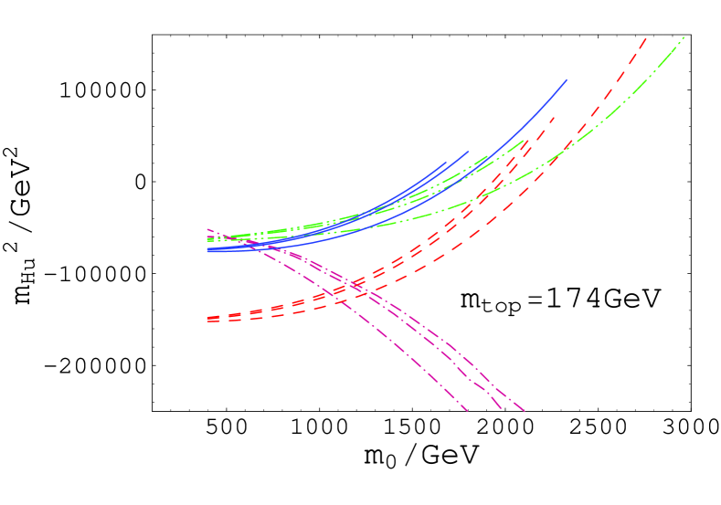
(b) $m_{t}=178$ GeV

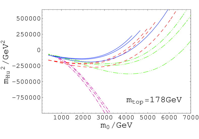
Figure 1: The $m_{0}$ dependence of $m_{H_{u}}^{2}$ at the stop mass scale $Q=Q_{\tilde{t}}$ for sgn$(\mu)=+1$ and for the top quark pole mass (a) $m_{t}=174$GeV or (b) $m_{t}=178$GeV. The blue (solid) lines correspond to $M_{1/2}=200$GeV and $A_{0}=0$GeV, the red (dashed) lines $M_{1/2}=300$GeV and $A_{0}=0$GeV, the green (dash-dot-dotted) lines $M_{1/2}=200$GeV and $A_{0}=0.5m_{0}$, and the purple (dash-dotted) lines $M_{1/2}=200$GeV and $A_{0}=m_{0}$. The three lines of each type correspond to $\tan\beta=10,20$, and $30$, respectively, from below.

In Fig.1, we show the $m_{0}$ dependence of $m_{H_{u}}^{2}$ at a typical stop mass scale $Q=Q_{\tilde{t}}=(m_{\tilde{t}_{1}}m_{\tilde{t}_{2}})^{1/2}$. In this computation, we impose the boundary condition $m_{scalar}^{2}=m_{0}^{2}$ at the GUT scale (i.e. $Q_{0}=M_{\rm GUT}$), and take a universal gaugino mass $M_{i}=M_{1/2}$, for simplicity. As expected, the value of $m_{H_{u}}^{2}$ is much suppressed compared to the corresponding $m_{0}^{2}$ for the case of $|M_{i}|\ll m_{0}$ and $|A_{0}|<m_{0}$. We have plotted it for two central values of the observed top quark pole mass $m_{t}$: one is extracted from the Particle Data Group [21] $m_{t}=174.3\pm 5.1$ GeV and the other from the recent CDF and D0 results [22] $m_{t}=178.0\pm 4.3$ GeV.

In the SSM, the parameter $\mu$ is related to the $Z^{0}$ boson mass $m_{Z^{0}}$ by minimizing the effective Higgs potential, and it can be expressed at the tree level as

$$\frac{1}{2}m_{Z^{0}}^{2}=\frac{m_{H_{d}}^{2}-m_{H_{u}}^{2}\tan^{2}\beta}{\tan^{2}\beta-1}-|\mu|^{2}\simeq{m_{H_{d}}^{2}\over\tan^{2}\beta}-m_{H_{u}}^{2}-|\mu|^{2}.$$ (13)

Thus, $m_{H_{u}}^{2}$ of the order of the gaugino masses manages to generate the electroweak symmetry breaking at the correct energy scale, or $m_{Z^{0}}=91.2$ GeV, with the $\mu$ parameter naturally implied by the GM term (10). Here, the parameters in Eq.(13) are regarded to be values at the electroweak scale, while the RG evolution of $\mu$ from the electroweak scale to the input scale is negligible in order estimation (see Eq.(18) in the Appendix).

(a) $m_{t}=174$ GeV

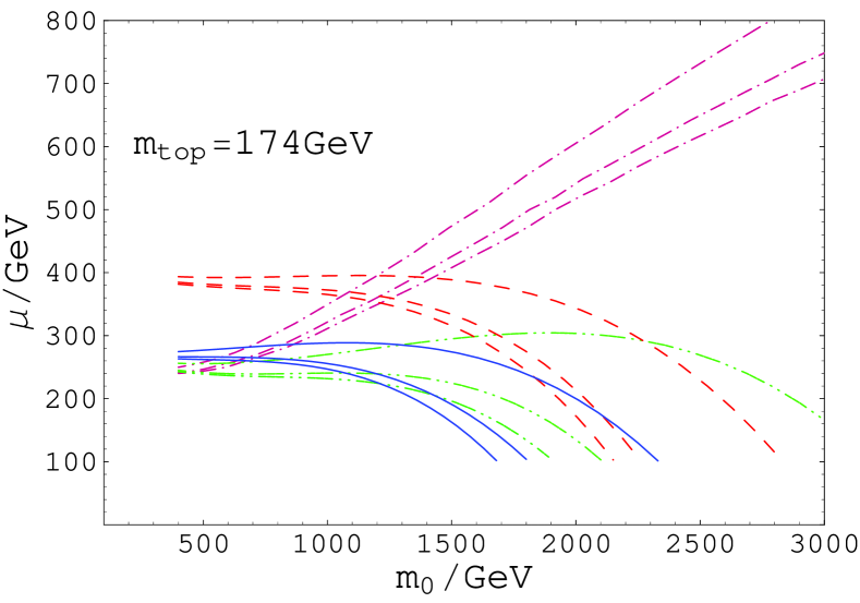
(b) $m_{t}=178$ GeV

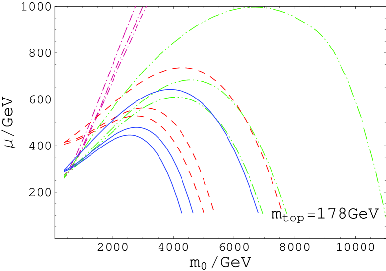
Figure 2: The $m_{0}$ dependence of $\mu$ at the stop mass scale $Q=Q_{\tilde{t}}$ for sgn$(\mu)=+1$ and for the top quark pole mass (a) $m_{t}=174$GeV or (b) $m_{t}=178$GeV. The notations for the lines are the same as in Fig.1, except for the corresponding values of $\tan\beta$ reversed in order: $\tan\beta=10,20$, and $30$ from above.

In Fig.2, we show admissible values of the $\mu$ parameter which yield the observed value of $m_{Z^{0}}=91.2$ GeV. To determine the value of $\mu$, we have used the ISAJET 7.69 code [23], which takes into account the one-loop corrections to the effective Higgs potential and the two-loop RG evolutions of parameters. The minimization of the effective Higgs potential is also performed at the typical stop mass scale $Q=Q_{\tilde{t}}$. We see that the value of $\mu$ should be much suppressed compared to $m_{0}$ for $|M_{i}|\ll m_{0}$, $|A_{0}|<m_{0}$ and hence it is consistent with our large-cutoff hypothesis.

Let us comment on the falling-off behavior of the allowed $\mu$ in the very large $m_{0}$ region in Fig.2. This behavior stems from a large cancellation between the suppressed $m_{0}^{2}$ contribution and the remaining ones to the value of the $\mu$ parameter. In such a region, the $\mu$ becomes very small due to the cancellation.

From a cosmological point of view, the parameter regions with tiny $\mu$ may provide a natural explanation for the observed dark matter density [25], since the lightest neutralino is a bino-Higgsino mixture for such regions and its relic abundance is in a cosmologically interesting range.

4.2 Consistency of the tree-level $B$ term

We have assumed the GM term as the origin of the $\mu$ parameter of the electroweak order. Then, the SUSY-breaking Higgs mixing parameter $B_{0}$ is related to the $A_{0}$ parameter at the input scale. For the term (10), the tree-level relation is given by [19]

$$B_{0}=B_{0}^{GM}\equiv\frac{2A_{0}-3m_{3/2}}{A_{0}-3m_{3/2}}m_{3/2}.$$ (14)

In this subsection, we examine how this condition is satisfied in the electroweak physics.

To study the matching condition Eq.(14), we take the following procedure: We first fix sampling values of $(m_{0},M_{i},A_{0},{\rm sgn}(\mu),\tan\beta)$, and determine the required values of $\mu$ and $B$ that reproduce $m_{Z^{0}}=91.2$ GeV. In addition to Eq.(13), we have a relation

$$B\mu=\frac{\sin 2\beta}{2}(m_{H_{u}}^{2}+m_{H_{d}}^{2}+2|\mu|^{2}),$$ (15)

which is also obtained by minimizing the tree-level effective Higgs potential. By means of Eqs.(13) and (15), we can obtain $\mu$ and $B$ at the electroweak scale for the given mSUGRA parameters. Then, from the value of $B$ at the electroweak scale, we compute the $B$ parameter at the input scale (i.e. $B_{0}$) and compare it with $B_{0}^{GM}$ in Eq.(14) to see whether or not the condition Eq.(14) is satisfied.

We find from Eq.(15) that the required value of $B$ at the electroweak scale is given by

$$B\sim\frac{m_{0}^{2}}{\mu\tan\beta},$$ (16)

since $m_{H_{d}}^{2}\sim m_{0}^{2}\gg|m_{H_{u}}^{2}|,\,|\mu|^{2}$ and $\sin 2\beta/2\simeq 1/\tan\beta$ for $\tan\beta\mathop{}_{\textstyle\sim}^{\textstyle>}10$.

(a) $m_{t}=174$ GeV

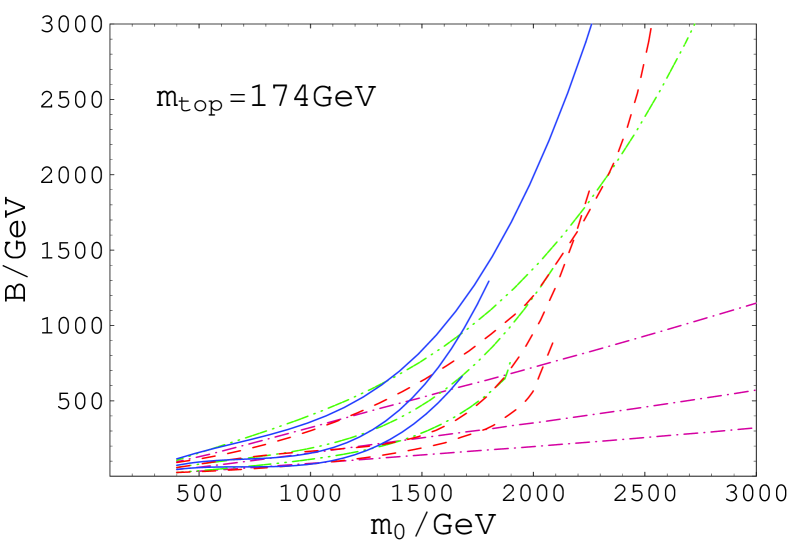
(b) $m_{t}=178$ GeV

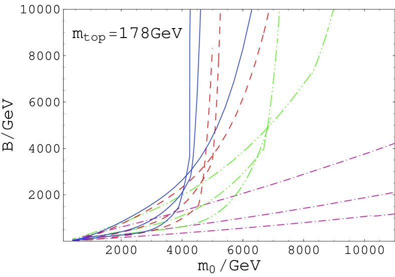
Figure 3: The $m_{0}$ dependence of $B$ at the stop mass scale $Q=Q_{\tilde{t}}$ for sgn$(\mu)=+1$ and for the top quark pole mass (a) $m_{t}=174$GeV or (b) $m_{t}=178$GeV. The notations for the lines are the same as in Fig.1.

In Fig.3, we show numerical results on the value of $B$ at the stop mass scale $Q=Q_{\tilde{t}}$ as a function of $m_{0}$. By comparing it with the $\mu$ parameter in Fig.2, we find that the value of $B$ becomes very large when the value of $\mu$ becomes very small, as expected from Eq.(16).

On the other hand, from the relation Eq.(14), we see $B_{0}^{GM}\sim m_{0}$ for $|A_{0}|<m_{0}=m_{3/2}$. Thus Eq.(16) implies that the condition Eq.(14) can be satisfied for $\mu\sim m_{0}/\tan\beta\ll m_{0}$, since the RG evolution of $B$ from the electroweak scale to the input scale is not significant: the RG equation of $B$ is controlled by relatively small $M_{i}$ and $A$ parameter contributions (see Eq.(19) in the Appendix), and thus $B\sim B_{0}$. As a result, we find that the condition Eq.(14) is satisfied in a certain parameter region.

(a) tan$\beta=20$

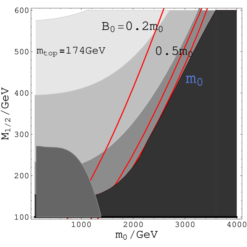
(b) tan$\beta=20$

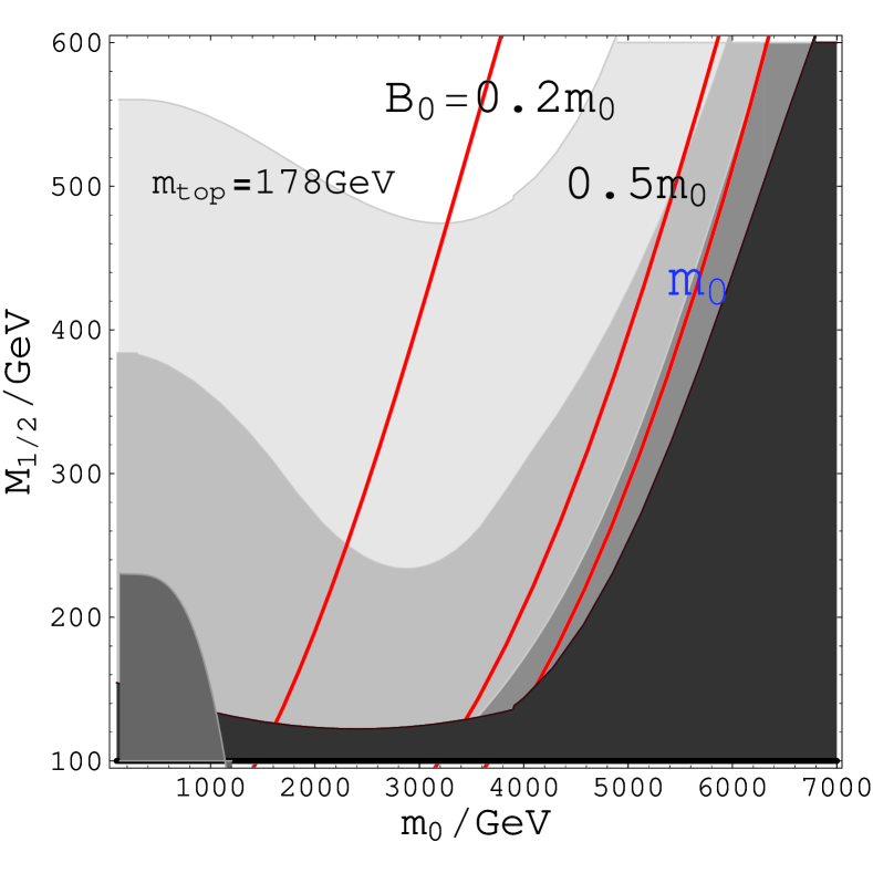
(c) tan$\beta=10$

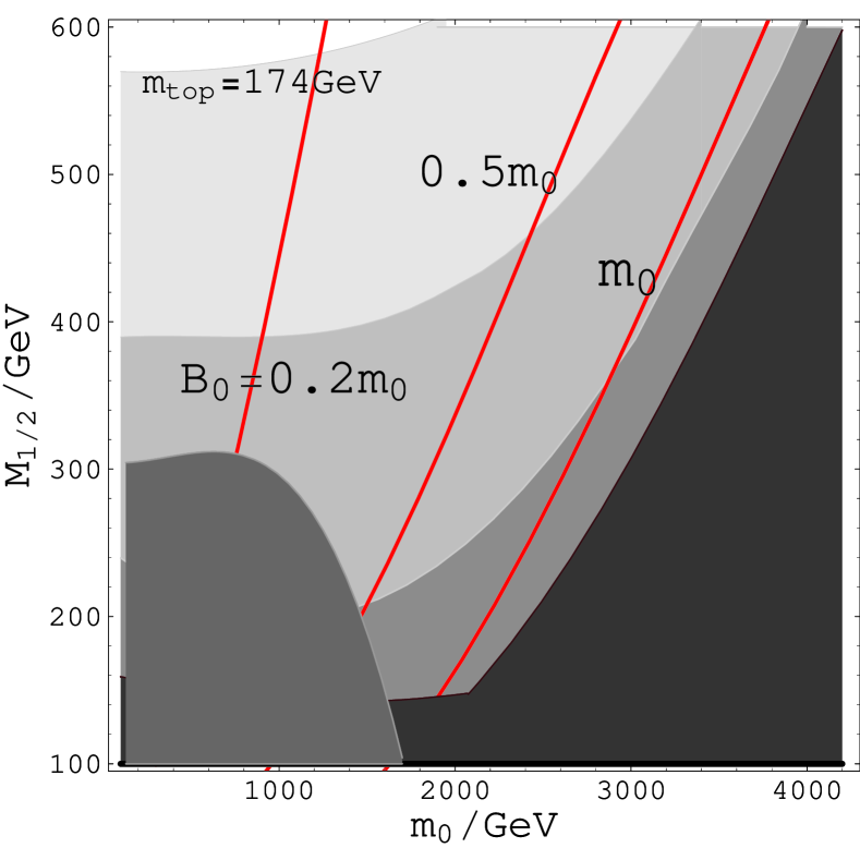
(d) tan$\beta=10$

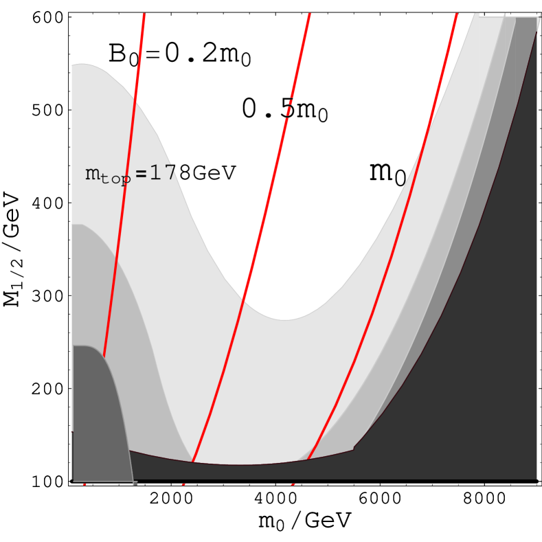
Figure 4: Contour plots for the required values of $B=B_{0}$ at the input scale $Q_{0}=M_{GUT}\simeq 2\times 10^{16}$GeV in the ($m_{0}$, $M_{1/2}$) plane for the top quark pole mass (a,c) $m_{t}=174$GeV or (b,d) $m_{t}=178$GeV and for (a,b) $\tan\beta=20$ or (c,d) $\tan\beta=10$. In all the panels, we have fixed $A_{0}=0$, sgn$(\mu)=+1$, and the red (solid) lines correspond to $B_{0}=0.2m_{0},0.5m_{0},m_{0}$, respectively, from the left to the right. The GM term implies the parameter regions on the $B_{0}=B_{0}^{GM}=m_{0}$ lines (see Eq.(15)). The gray shaded regions correspond to the parameters where the required value of $\mu$ is smaller than $700$GeV, $500$GeV, and $300$GeV, respectively, from above. The dark shaded regions at the bottom-left represent the Higgs mass bound $114$ GeV[27], and the black shaded regions are excluded by the chargino mass limit, $m_{\chi^{\pm}}\geq 104$GeV [28].

(a) tan$\beta=5$

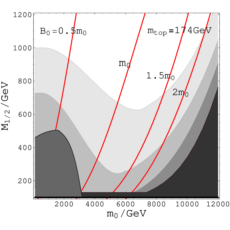
(b) tan$\beta=5$

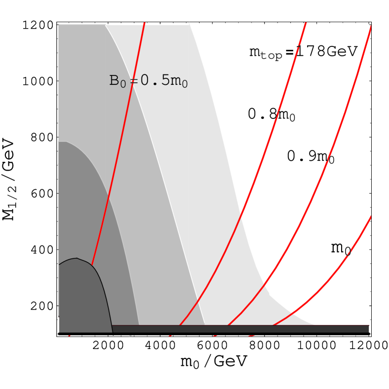
(c) tan$\beta=4$

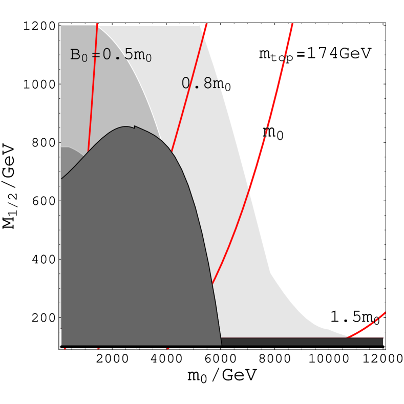
(d) tan$\beta=4$

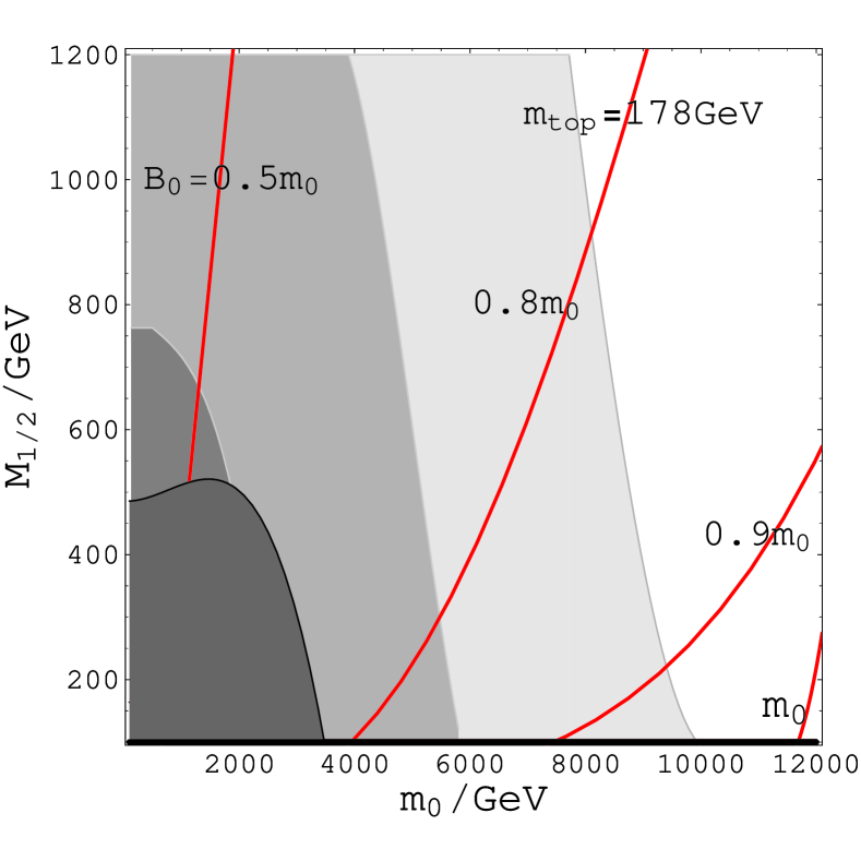
Figure 5: Contour plots for the required values of $B=B_{0}$ at the input scale $Q_{0}=M_{GUT}\simeq 2\times 10^{16}$GeV in the ($m_{0}$, $M_{1/2}$) plane for the top quark pole mass (a,c) $m_{t}=174$GeV or (b,d) $m_{t}=178$GeV and for (a,b) $\tan\beta=5$ or (c,d) $\tan\beta=4$. In all the panels, we have fixed $A_{0}=0$, sgn$(\mu)=+1$, and the red (solid) lines correspond to $B_{0}$ fixed as indicated. The GM term implies the parameter regions on the $B_{0}=B_{0}^{GM}=m_{0}$ lines (see Eq.(15)). The gray shaded regions correspond to the parameters where the required value of $\mu$ is smaller than $1200$GeV, $900$GeV, and $600$GeV from above in the panel (a); smaller than $2000$GeV, $1500$GeV, and $1000$GeV from the right in the panels (b,c); and smaller than $3000$GeV, $2000$GeV, and $1000$GeV from the right in the panel (d). The dark shaded regions at the bottom-left represent the Higgs mass bound $114$GeV [27], and the black shaded regions are excluded by the chargino mass limit, $m_{\chi^{\pm}}\geq 104$GeV [28].

In Figs.4 and 5, we plot the contours of the values of $B_{0}$ at the input scale $Q_{0}=M_{GUT}$ on the $(m_{0},M_{1/2}\geq 0)$ plane with the fixed values of $A_{0}=0$, sign$(\mu)=+1$, and $\tan\beta=20,10,5,4$ as demonstrations. In the figures, we also show the value of $\mu$ at the stop mass scale $Q=Q_{\tilde{t}}$.

Before examining the contours of $B_{0}$, let us first understand the behavior of $\mu={\rm constant}$ lines in the figures. Generic behavior of the $\mu={\rm constant}$ lines may be seen from the panels (b,d) in Fig.4 and (a) in Fig.5. The lines are elliptic in small $m_{0}$ regions (elliptic domains) and hyperbolic in large $m_{0}$ regions (hyperbolic domains). They are parabolic in between (parabolic domains), where the value of $\mu$ is relatively insensitive to the variation of $m_{0}$ with $M_{1/2}$ fixed. In this perspective, the panels (a,c) in Fig.4 belong to hyperbolic domains (continued from parabolic domains), where the $\mu={\rm constant}$ lines are hyperbolae (in the large $\tan\beta$ case in Ref.[4]); and the panels (b,c,d) in Fig.5 belong to elliptic domains (continued on parabolic domains), where the $\mu={\rm constant}$ lines are ellipses (in the small $\tan\beta$ case in Ref.[4]). We note that such behavior may be obtained from Eqs.(11), (12), and (13) with the stop mass as the renormalization scale $Q=Q_{\tilde{t}}\sim m_{0}$.

Now, by inspection of $B_{0}=B_{0}^{GM}=m_{0}$ lines due to the GM term (10) for $A_{0}=0$ (see Eq.(15)) in the figures, it is apparent that the large-cutoff theories with $m_{0}\gg|M_{1/2}|,|\mu|$ correspond to those lines along the hyperbolic domains in Fig.4 with moderate $\tan\beta$. In particular, the lower ends of the $B_{0}=m_{0}$ lines are in small $M_{1/2}$ regions with $m_{0}$ of a few TeV, which may be within the reach of accelerator experiments in the near future.

More generally, the figures imply that, in the large-cutoff theory, the tree-level relation of the GM term (10) in mSUGRA can be satisfied for various parameters with $m_{0}\gg|M_{i}|,|\mu|$, which are consistent with the present observational bounds. Hence we conclude that the GM term works very well with our large-cutoff hypothesis.

5 Conclusions and Discussion

Gravity-mediated supersymmetry breaking and primordial inflation are expected to open windows into the Planck-scale physics through observations on superpartner spectra [1] and on temperature fluctuations of cosmic microwave background radiation [13]. In this paper, we have discussed realization of the large-cutoff theory in supergravity, which is possibly selected through inflationary dynamics. This large-cutoff hypothesis implies an mSUGRA spectrum with a large hierarchy between the universal scalar mass and the gaugino masses, $m_{0}\gg|M_{i}|$. Very encouragingly, despite of relatively large masses of scalar particles, the electroweak symmetry breaking can occur at the correct energy scale with $m_{0}\gg|\mu|$ in phenomenologically viable parameter regions.

In the large cutoff hypothesis, the absence of the FCNC process is automatic, since all of the corresponding higher dimensional operators in the Kähler potential are suppressed by the large cutoff $M_{*}$. In addition, with the current chargino mass bound, the hierarchical spectrum $m_{0}\gg|M_{i}|,|\mu|$ predicts heavy sfermions at a few TeV, and hence the CP problem in the SSM is ameliorated. In most of the parameter region ($m_{0}\gg|M_{i}|,|\mu|$) we are interested in, the lightest supersymmetric particle is a neutralino, which is a good candidate for the dark matter (see also the remark at the end of section 4.1).

Finally, let us comment on the origin of matters in the universe in the present scenario. The hierarchical spectrum implies that the mass of the gravitino is of the order of a few TeV. In this case, the primordial abundance of the gravitino should be suppressed not to disturb the Big-Bang Nucleosynthesis, which implies the reheating temperature $T_{R}\mathop{}_{\textstyle\sim}^{\textstyle<}$ $10^{6-7}$ GeV [29]. Hence, the baryon asymmetry must be provided at the corresponding low temperatures, $T\mathop{}_{\textstyle\sim}^{\textstyle<}$ $10^{6-7}$ GeV.

Appendix: Notation for the Higgs Potential

In this appendix, we list our convention for the Higgs mass parameters. We adopt the following form of the effective Higgs potential at the tree level:

$$V = (|\mu|^{2}+m_{H_{u}}^{2})(|H_{u}^{0}|^{2}+|H_{u}^{+}|^{2})+(|\mu|^{2}+m_{H_{d}}^{2})(|H_{d}^{0}|^{2}+|H_{d}^{+}|^{2})$$ (17)

$$+B\mu\left\{(H_{u}^{+}H_{d}^{-}-H_{u}^{0}H_{d}^{0})+c.c.\right\}+\frac{1}{2}g^{2}|H_{u}^{+}H_{d}^{0*}+H_{u}^{0}H_{d}^{-*}|^{2}$$

$$+\frac{1}{8}(g^{2}+g^{\prime 2})(|H_{u}^{0}|^{2}+|H_{u}^{+}|^{2}-|H_{d}^{0}|^{2}-|H_{d}^{+}|^{2})^{2},$$

where the superscript $(0,+,-)$ of each field denotes its electric charge, and $g$ and $g^{\prime}$ denote the $SU(2)_{W}$ and $U(1)_{Y}$ gauge coupling constants, respectively. With this convention, the RG equations for the $\mu$ and $B$ parameters are given at the one-loop level by

$$\frac{d}{d\ln Q}\mu = \frac{\mu}{16\pi^{2}}(3|y_{t}|^{2}+3|y_{b}|^{2}+|y_{\tau}|^{2}-3g^{2}-g^{\prime 2}),$$ (18)

$$\frac{d}{d\ln Q}B = \frac{1}{16\pi^{2}}(6A_{t}|y_{t}|^{2}+6A_{b}|y_{b}|^{2}+2A_{\tau}|y_{\tau}|^{2}+6g^{2}M_{2}+2g^{\prime 2}M_{1}),$$ (19)

where $A_{i}\cdot y_{i}$ $(i=t,b,\tau)$ denotes the (scalar)³ coupling constant that is the supersymmetric counterpart of the Yukawa coupling $y_{i}$ for each flavor $t,b$, or $\tau$.

References

-
[1]
For reviews, H.P. Nilles, Phys. Rept. 110 (1984) 1;
D.J.H. Chung, L.L. Everett, G.L. Kane, S.F. King, J. Lykken, and L.-T. Wang, arXiv:hep-ph/0312378. - [2] Izawa K.-I. and T. Yanagida, arXiv:hep-ph/9809366; arXiv:hep-ph/9904426.
- [3] R. Barbieri and G.F. Giudice, Nucl. Phys. B306 (1988) 63.
- [4] K.L. Chan, U. Chattopadhyay, and P. Nath, arXiv:hep-ph/9710473.
- [5] J.L. Feng, K.T. Matchev, and T. Moroi, arXiv:hep-ph/9908309; arXiv:hep-ph/9909334.
- [6] R. Bousso and J. Polchinski, arXiv:hep-th/0004134.
- [7] See also L. Smolin, arXiv:hep-th/0407213, and references therein.
- [8] Izawa K.-I., Prog. Theor. Phys. 86 (1991) 917.
- [9] A. Vilenkin, arXiv:gr-gc/9406010.
- [10] Izawa K.-I. and T. Yanagida, arXiv:hep-ph/9608359.
- [11] Izawa K.-I., arXiv:hep-ph/0305286.
-
[12]
Izawa K.-I. and T. Yanagida, arXiv:hep-th/9602180;
T. Hotta, Izawa K.-I., and T. Yanagida, arXiv:hep-ph/9606203;
Izawa K.-I., Y. Nomura, K. Tobe, and T. Yanagida, arXiv:hep-ph/9705228;
Izawa K.-I., arXiv:hep-ph/9708315. -
[13]
For reviews, D.H. Lyth and A. Riotto, arXiv:hep-ph/9807278;
W.H. Kinney, arXiv:astro-ph/0301448;
S.F. King, arXiv:hep-ph/0304264. -
[14]
E. Witten and J. Bagger, Phys. Lett. B115 (1982)
202;
M.K. Gaillard, arXiv:hep-th/9806227. -
[15]
M.K. Gaillard and V. Jain, arXiv:hep-th/9308090;
M.K. Gaillard, arXiv:hep-th/9408149;
K. Choi, J.S. Lee, and C. Muñoz, arXiv:hep-ph/9709250. -
[16]
Izawa K.-I., M. Kawasaki, and T. Yanagida,
arXiv:hep-ph/9707201;
Izawa K.-I., arXiv:hep-ph/9710479. - [17] See M. Dine and D.A. MacIntire, arXiv:hep-ph/9205227.
- [18] Izawa K.-I. and T. Yanagida, arXiv:hep-ph/9507441.
- [19] G.F. Giudice and A. Masiero, Phys. Lett. B206 (1988) 480.
- [20] S. Codoban and D.I. Kazakov, arXiv:hep-ph/9906256.
- [21] S. Eidelman et al., Phys. Lett. B592 (2004) 1.
- [22] P. Azzi et al., arXiv:hep-ex/0404010.
- [23] F.E. Paige, S.D. Protopescu, H. Baer, and X. Tata, arXiv:hep-ph/0312045.
- [24] B.C. Allanach, S. Kraml, and W. Porod, arXiv:hep-ph/0302102.
- [25] J.L. Feng, K.T. Matchev, and F. Wilczek, arXiv:hep-ph/0004043.
- [26] J.R. Ellis, K.A. Olive, Y. Santoso, and V.C. Spanos, arXiv:hep-ph/0405110.
- [27] G. Abbiendi et al., arXiv:hep-ex/0306033.
- [28] LEP2 SUSY Working Group, Combined LEP Chargino Results, up to GeV for large m0, http://lepsusy.web.cern.ch/lepsusy/www/inos_moriond01/charginos_pub.html.
- [29] For recent developments, M. Kawasaki, K. Kohri and T. Moroi, arXiv:astro-ph/0408426.