Glueball Regge trajectories and the Pomeron
– a lattice study –
Harvey B. Meyer and Michael J. Teper

Rudolf Peierls Centre for Theoretical Physics,

University of Oxford,

1 Keble Road, Oxford OX1 3NP, U.K.

Abstract

We perform lattice calculations of the lightest $J=0,2,4,6$ glueball masses in the D=3+1 SU(3) gauge theory and extrapolate to the continuum limit. Assuming that these masses lie on linear Regge trajectories we find a leading glueball trajectory $\alpha(t)=0.93(24)+0.28(2)\alpha^{\prime}_{R}t$, where $\alpha^{\prime}_{R}\simeq 0.9\,\mathrm{GeV}^{-2}$ is the slope of the usual mesonic Regge trajectory. This glueball trajectory has an intercept and slope similar to that of the Pomeron trajectory. We contrast this with the situation in D=2+1 where the leading glueball Regge trajectory is found to have too small an intercept to be important for high-energy cross-sections. We interpret the observed states and trajectories in terms of open and closed string models of glueballs. We discuss the large-$N$ limit and perform an SU(8) calculation that hints at new states based on closed strings in higher representations.

1 Introduction

The experimentally observed mesons and baryons appear to lie on nearly linear and parallel Regge trajectories,

$$J\equiv\alpha(t=m^{2})\simeq\alpha_{0}+\alpha^{\prime}m^{2}$$ (1)

with $\alpha^{\prime}\simeq 0.9\,\mathrm{GeV}^{-2}$ and $\alpha_{0}\leq 0.5$. The exchange of the highest-lying Regge pole will dominate any high energy scattering that involves the exchange of the corresponding quantum numbers (see e.g. [1] for a recent review).

The total cross-section, on the other hand, is related by unitarity to forward elastic scattering and this is dominated by the ‘Pomeron’ which carries vacuum quantum numbers [1, 2, 3]. The Pomeron trajectory is qualitatively different from other Regge trajectories in that it is much flatter ($\alpha^{\prime}$ much smaller) and has a higher intercept [3]

$$\alpha_{P}(t=m^{2})\simeq 1.08+0.25m^{2}$$ (2)

(in GeV units). A unit intercept would lead to total cross-sections that are constant with energy. The fact that cross-sections increase slowly with energy suggests an intercept slightly larger than unity. Since it does not seem possible to associate the Pomeron with the usual flavour-singlet mesons (whose leading trajectory would have the usual slope and too low an intercept) there has been a long-standing speculation that the physical particles on the trajectory (at integer values of the spin $J$) might be glueballs. This picture arises naturally in string models of hadrons.

If we now consider the high-energy scattering of glueballs in the pure SU(3) gauge theory, it is difficult to imagine that the total cross-section should behave differently from total cross-sections in the real world. For instance, in leading-logarithmic perturbative calculations ([2] and ref. therein), only the gluonic field contributes to the Pomeron. Thus it is reasonable to expect that the Pomeron will appear in the pure gauge theory, with similar properties to those of the phenomenological Pomeron (up to corrections due to effects such as mixing). This constitutes the main motivation for the calculations of this paper in which we use numerical lattice techniques to investigate whether the mass spectrum of the SU(3) gauge theory is consistent with approximately straight Regge trajectories, the leading one of which possesses the properties of the phenomenological Pomeron.

The states that lie on the phenomenological Pomeron will have even spin (the trajectory has even signature) and will start with $J=2$ since the high intercept implies that $m^{2}<0$ for $J=0$ so that the lightest $J=0$ state must lie on a daughter trajectory. Thus we need to calculate the lightest masses with $J=2$ and $J=4$, and preferably $J=6$ as well. There are two major obstacles to this. The first arises from the reduced rotational invariance of the cubic lattice, which makes the identification of states with $J\geq 4$ a non-trivial problem. In [4], we developed a technique to label highly excited states from the lattice with the correct spin $J$ and we applied it in the simpler context of 2+1 dimensional $SU(N)$ gauge theories [5]. We have now extended this technique to three space dimensions and will use it in this paper. The technical details are left to a longer publication [6]. The second obstacle is that the higher spin states are much more massive and therefore difficult to calculate accurately by the standard numerical methods. We therefore apply recent algorithmic improvements [7, 8] that help reduce the variance of rapidly decaying correlators.

In the next Section we summarise the results of our lattice calculation of the $PC$=++ sector of the glueball spectrum and identify the leading and sub-leading glueball Regge trajectories. We find that the former does indeed possess the qualitative features of the Pomeron. To show how things might have been different, we also summarise the results of a similar calculation in $D=2+1$ where one finds a leading glueball trajectory that has a very low intercept. We then turn to a discussion of the string picture of mesons and glueballs, which provides the framework within which we interpret our results for the glueball mass spectrum. (This is what one would now refer to as the ‘old’ string picture for QCD; for relevant work within the ‘new’ string picture, see [9] and references therein.) We first remind the reader how the usual mesonic Regge trajectories can be understood within a simple string model of quarkonia, and how this picture naturally translates to glueballs in the pure gauge theory. We emphasise the richer structure that this predicts for the associated glueball Regge trajectories, and we use the observed pattern of states and degeneracies to associate the observed trajectories with specific kinds of open and closed strings. As well as discussing the well-established Pomeron trajectory, we use our calculated spectrum to comment upon the more speculative $C$=$-$ odderon (for a review see [10]). Finally we comment upon the SU($N\to\infty$) limit and some implications for the high energy scattering of glueballs and hadrons.

This paper is a summary of the results of calculations that will be described in detail in a longer paper [6]. In particular the reader is referred to that paper for the technical details of our lattice calculations as well as for a more detailed exploration of what string models predict for glueballs and for comments on earlier lattice calculations of higher spin glueballs.

2 Results for the $PC=++$ glueball spectrum.

Our lattice calculations employ the standard plaquette action. We calculate ground and excited state masses, $m$, from Euclidean correlation functions using standard variational techniques. We calculate the string tension, $\sigma$, by calculating the mass of a flux loop that closes around a spatial torus. We perform calculations for values of the inverse bare coupling $\beta=6/g^{2}$ ranging from $\beta=6.0$ to $\beta=6.4$, which corresponds to lattice spacings $a\simeq 0.10-0.05\,\mathrm{fm}$. The calculations are on lattices ranging from $16^{3}36$ to $32^{3}48$, corresponding to a spatial extent $aL\simeq 1.5\,\mathrm{fm}$. At one value of $\beta$ we perform calculations on lattices up to $2\,\mathrm{fm}$ across so as to check that any finite volume corrections are small. We extrapolate the calculated values of the dimensionless ratio $m/\surd\sigma$ to $a=0$ using an $a^{2}\sigma$ correction, which is the leading correction with the plaquette action. We thus obtain the continuum glueball spectrum with masses expressed in units of the string tension. All this is quite standard (see e.g. [11]).

There are two novel aspects to our calculations. The first is a recently developed variance reduction technique [7, 8] that is very useful for reducing statistical errors on masses that are large, such as those of the higher spin states in which we shall be interested. The second is the identification of the lightest $J\geq 4$ states. The problem is that the cubic rotation group of the lattice is much smaller than the continuum rotation group and has just a few irreducible representations. Nonetheless this does not mean that it makes no sense to label states by their ‘spin $J$’. As $a\to 0$ an energy eigenstate belonging to one of these lattice representations will tend to some state that is labelled by spin $J$. So using continuity we can refer to a state at finite $a$ as being of ‘spin $J$’ if $a$ is small enough. (Level crossings at large $a$ may eventually render such a labelling ambiguous.) At $a=0$ a state of spin $J$ will appear in a multiplet of $2J+1$ degenerate states. If we now increase $a$ from zero, these $2J+1$ states will in general appear in different lattice representations, and the degeneracy will be broken at $O(a^{2})$. So in general the ground state of spin $J=4,5,6,...$ will be a (highly) excited state in some lattice representation, thus complicating its identification. If we can perform this identification, then we can extrapolate the mass of the state to $a=0$, so obtaining the mass of, say, the lightest state of spin $J$. Our identification technique, as described in [4] for the simpler case of $D=2+1$, is to perform a Fourier transform of the rotational properties of any given lattice eigenstate, using as a probe a set of lattice operators that have an approximate rotational symmetry that is greater than the exact cubic symmetry, so that we can probe rotational properties under rotations finer than $\pi/2$. If we find that the state has predominantly the rotational properties corresponding to say $J=4$, and if we find that this predominance grows towards unity as $a\to 0$, then we can assign to it these continuum rotational quantum numbers. In addition there should be states corresponding to the other members of the spin multiplet that become degenerate with it as $a\to 0$, and this provides extra evidence for the correctness of the spin assignment. (The density of states and the errors on masses prevents us from using this degeneracy as the sole criterion in practice.)

The technical details of these methods will be provided elsewhere [6]. We now turn to a summary of our results.

2.1 Glueball Regge trajectories in D=3+1

Figure 1: Chew-Frautschi plot of the continuum 4D $SU(3)$ gauge theory. The hyperbolae are drawn to suggest the behaviour of the two leading trajectories. The position of some experimental flavour-singlet mesons is indicated [19].

Figure 2: The Chew-Frautschi plot of the continuum D=2+1 $SU(3)$ glueball spectrum.

We initially focus on states with $PC$=++ since these are the quantum numbers carried by the Pomeron.

Extrapolating our glueball masses to the continuum limit we plot the (squared) masses against the spins in a Chew-Frautschi plot, as in Fig.1. We now assume that the states fall on approximately linear Regge trajectories. (To obtain significant evidence for or against such linearity would require more accurate $J=6$ masses than we have been able to achieve in the present calculation.) In that case the leading trajectory clearly passes through the lightest $J=2$ and $J=4$ glueballs (and within about one standard deviation of the lightest $J=6$ glueball). We note that there is no odd $J$ state on this trajectory: it is even signature just like the phenomenological Pomeron. The parameters of the trajectory are

$$2\pi\sigma\alpha^{\prime}=0.281(22)\qquad\alpha_{0}=0.93(24).$$ (3)

which is entirely consistent with the phenomenological Pomeron in Eq. (2), if we recall that the usual mesonic trajectories have slopes

$$\alpha^{\prime}_{\cal R}\simeq\frac{1}{2\pi\sigma}\simeq 0.9\,\mathrm{GeV}^{-2}.$$ (4)

Of course, in comparing our leading pure-glue trajectory with the phenomenological Pomeron we should not ignore the fact that the latter will mix with the flavourless mesonic trajectory, shown in Fig.1. It is plausible that the mixing will effectively increase the intercept and the slope of the Pomeron. In particular it might well be that the underlying unmixed pure-gauge Pomeron has an intercept of 1 rather than $\sim 1.08$.

We can also identify in Fig.1 the sub-leading glueball trajectory. It contains the lightest $J=0$ glueball, the first excited $J=2$ glueball and the lightest $J=3$ glueball. Our lower bound on the mass of the lightest $J^{PC}=1^{++}$ makes it clear that it is much too heavy to lie on this trajectory. We remark that we have not identified any excited $J=4$ or $J=5$ states, with $PC=++$, and so cannot say whether they lie on this trajectory or not. In striking contrast to what one finds for the usual mesonic trajectories, this secondary trajectory is clearly not parallel to the leading one. As we shall see in the next Section, this is something one might expect within a string picture of glueballs. The trajectories cross somewhere near $J=5$ and it is not quite clear to which trajectory the observed $J=6$ state belongs. Clearly it would be useful to have a mass estimate for the first excited $J=6$ state. Finally we remark that because of unitarity the trajectories will not actually cross but will rather repel, as indicated in Fig. 1.

We thus conclude that the leading Regge trajectory in the pure SU(3) gauge theory does indeed appear to be the ‘bare’ Pomeron, which will become the phenomenological Pomeron after mixing with the appropriate mesonic Regge trajectory. We now turn to a similar analysis for the SU(3) gauge theory in $D=2+1$, which will demonstrate that there is nothing inevitable about our above result.

2.2 Glueball Regge trajectories in D=2+1

In Fig.2 we show the Chew-Frautschi plot for the $C=+$ sector of the continuum SU(3) gauge theory in $D=2+1$. (We do not refer to parity, because in two space dimensions one has automatic parity-doubling for $J\not=0$.) In contrast to $D=3+1$, a linear trajectory between the lightest $J=2$ and $J=4$ states passes through the lightest $J=0$ state, and so we should place the $J=0$ glueball on that trajectory. Between them the $J=0,2,4$ states provide strong evidence for the approximate linearity of the trajectory. In contrast to $D=3+1$ the secondary trajectory is approximately parallel to the leading one.

It is clear from Fig.2 that the intercept is very low, so that the leading glueball trajectory will make a contribution to the total cross-section that decreases rapidly with energy. Thus if the glueball-glueball total cross-section is approximately constant at high energies, then it will have to be understood in terms of something other than a Regge trajectory.

The parameters of the leading trajectory are

$$2\pi\sigma\alpha^{\prime}=0.384(16)\qquad\alpha_{0}=-1.144(71).$$ (5)

Thus, in contrast to the intercept, the slope of the trajectory is not very different from what we found in $D=3+1$.

3 String models

The string picture of hadrons starts from the observation that linear confinement implies that the flux between static charges is contained within a flux tube whose width will be on the order of $1/\surd\sigma$. Once this flux tube is long enough, $l\gg 1/\surd\sigma$, it will look like a string and this has led to a long-standing conjecture that the long-distance properties of QCD are given by some effective string theory.

The fact that mesons fall on nearly linear and parallel Regge trajectories reinforces this picture. A natural model for a high $J$ meson is to see it as a rotating string with a $q$ and $\bar{q}$ at its ends and, as is well-known (see e.g. [12]), a simple classical calculation shows how this leads to linear Regge trajectories with a slope determined by the string tension $\sigma$ (the rest energy per unit length of the string),

$$J\stackrel{{\scriptstyle J\to\infty}}{{=}}\frac{1}{2\pi\sigma}m^{2}+...$$ (6)

The value of the confining string tension that this requires, in order to produce the observed Regge slope, is consistent with the string tension one needs for the linear part of the heavy-quark potential and with the value that has been obtained in numerical simulations of quenched and full QCD (when expressed, for example, in units of the calculated $\rho$ meson mass or the nucleon mass).

If we now go to the pure gauge theory, this simple ‘open string’ model has an immediate analogue; two gluons joined by a string containing flux in the adjoint representation. However, in contrast to the case of mesons, there is an alternative closed string model: a closed string of flux in the fundamental representation. We now discuss and contrast these two models in more detail.

3.1 Open strings

We would expect a state of high spin to be highly extended, and in a confining theory this immediately suggests an open string. For mesons the string ends on quarks and carries fundamental flux, while for glueballs it ends on gluons and carries adjoint flux. Such an adjoint string can break through gluons popping out of the vacuum, but this is also true of the mesonic string (through $q{\bar{q}}$ popping out of the vacuum). What is important for the model to make sense is that the decay width should be sufficiently small – essentially that the lifetime of the adjoint string should be much longer than the period of rotation. In $SU(N)$ gauge theories, both the adjoint and fundamental strings become completely stable as $N\to\infty$. So if we are close to that limit the model can make sense. Indeed adjoint string breaking in $SU(N)$ occurs at $O(1/N^{2})$ while fundamental string breaking in $QCD_{N}$ occurs at $O(1/N)$. Thus a priori the adjoint string model can be taken at least as seriously as the conventional mesonic string model.

By the same classical calculation as used for mesons, the rotating adjoint string will produce a linear Regge trajectory

$$J\stackrel{{\scriptstyle J\to\infty}}{{=}}\frac{1}{2\pi\sigma_{A}}m^{2}+...\simeq\frac{1}{4.5\pi\sigma}m^{2}+...$$ (7)

where we have used the observed fact [13] that the adjoint and fundamental string tensions are related by Casimir scaling, $\sigma_{a}\simeq\frac{9}{4}\sigma$ for $N=3$. This gives a slope $\alpha^{\prime}\simeq 0.4\,\mathrm{GeV}^{-2}$ which is very much flatter than the usual mesonic Regge trajectory, although not quite as flat as the phenomenological Pomeron or the leading glueball trajectory we identified in Section 2.1.

Since the adjoint string comes back to itself under $C$, $P$ or rotations of $\pi$, we expect its spectrum to contain $J$ even and $P,C$ positive i.e.

$$J^{PC}=0^{++},2^{++},4^{++},...$$ (8)

just as one expects for an even-signature Pomeron.

3.2 Closed strings

Figure 3: The leading phononic and orbital Regge trajectories in the flux-tube model in 3+1D (with the bosonic string Casimir energy correction). The straight lines are semi-classical approximations to the trajectories. Crosses, circles and squares indicate the position of physical states with the corresponding quantum numbers.

For mesons an open string is the only natural string model. For glueballs, however, an equally natural model is one composed of a closed loop of fundamental flux with no constituent gluons at all. This should not be regarded as an alternative model. Rather one expects some glueball states to be open strings and others to be closed strings. (With mixing between the two, at finite $N$.) Clearly we would like to identify which state corresponds to which type of string.

An approximate but tractable closed string model was constructed in [14]. In this model the essential component is a circular closed string (flux tube) of radius $\rho$. There are phonon-like excitations of this closed string which move around it clockwise or anticlockwise and contribute to both its energy and its angular momentum. The system is (first) quantised so that we can calculate, from a Schrödinger-like wave equation [14], the amplitude for finding a loop in a particular radius interval. The phonon excitations are regarded as ‘fast’ so that they contribute to the potential energy term of the equation and the phonon occupation number is a quantum number labelling the wave-function. The whole loop can rotate around its diameter, obtaining angular momentum that way as well.

We refer the reader to [6] for the details of our analysis of this model. Here we simply state that if one considers the set of states where the angular momentum is purely phononic one obtains an asymptotically linear Regge trajectory with slope

$$J=\alpha(t=m^{2})\stackrel{{\scriptstyle J\to\infty}}{{=}}\frac{1}{8\pi\sigma}m^{2}+...$$ (9)

while for a loop with purely orbital motion one obtains a linear trajectory with

$$J=\alpha(t=m^{2})\stackrel{{\scriptstyle J\to\infty}}{{=}}\frac{3\surd 3}{32\pi\sigma}m^{2}+...$$ (10)

In either case one obtains a slope $\alpha^{\prime}\simeq 0.2-0.3\,\mathrm{GeV}^{-2}$ which is in the right range for the Pomeron. One can also calculate the intercept obtained by linearly extrapolating this trajectory from large to small $J$ but this depends on both the string ‘Casimir energy’ correction and on any curvature term in the effective string action. As an illustration we show in Fig.3 the Chew-Frautschi plot obtained by a numerical solution of the model (with a conventional string Casimir energy and no curvature term).

For the orbital trajectory, the geometry of the circular loop automatically gives it positive parity $P=+$. Furthermore, the mere fact that an oriented planar loop is spinning around an axis contained in its plane implies that the charge conjugation is determined by the spin:

$$P~{}=~{}+,\quad C~{}=~{}(-1)^{J},\quad J=0,1,2\dots$$ (11)

For the leading phononic trajectory, the most obvious feature is the absence of a $J=1$ state, because there is no corresponding phonon (it amounts to a mere translation). Secondly, for a planar loop, parity has the same effect as a $\pi$-rotation around an axis orthogonal to its plane. Therefore for phonons that lie in the plane of the loop

$$P~{}=~{}(-1)^{J},\quad C=\pm\quad J=0,2,3,4,\dots$$ (12)

while for phonons corresponding to fluctuations orthogonal to that plane:

$$P~{}=~{}(-1)^{J+1},\quad C=\pm\quad J=0,2,3,4,\dots$$ (13)

3.3 Other topologies

It is conceivable that for those quantum numbers for which the simple flux-tube model predicts a very large mass, other topologies of the string provide ways to construct a lighter fundamental state. A new pattern of quantum numbers arises if the oriented closed string adopts a twisted, ‘8’ type configuration, whilst remaining planar. The parity of such an object is automatically locked to the charge conjugation quantum number, $P=C$. The orbital trajectory built on such a configuration leads to a sequence of states

$$0^{++},~{}1^{--},~{}2^{++},~{}3^{--},~{}4^{++},~{}\dots$$ (14)

More exotic topologies of the string have been advocated in [15], but they presumably lead to more massive states. Such objects are more likely to be relevant to the large $N$ limit, where they will not decay.

3.4 String models in D=2+1

The SU(3) gauge theory in $D=2+1$ is linearly confining and therefore an effective string theory description is equally well motivated. Since the rotating open string lies in a plane, it provides a natural model for glueballs in two space dimensions. The closed string is also a possibility, although now all the angular momentum must come from phonons in the plane of the loop.

The open adjoint string will contribute states with $J$ even and $C=+$, just as in Eq. (8) except for the additional trivial parity doubling of non-zero spin states in two space-dimensions.

For the closed string, the quantum numbers for the leading $C=+$ and $C=-$ phononic trajectories are

$$J^{PC} = 0^{++},~{}2^{P+},~{}3^{P+},~{}4^{P+},~{}\dots\quad C=+$$

$$J^{PC} = 0^{--},~{}2^{P-},~{}3^{P-},~{}4^{P-},~{}\dots\quad C=-,$$

where $P$ is arbitrary, again because of the $J\not=0$ parity doubling. In the simplest form of the model, the two trajectories are degenerate.

We remark that an orbital trajectory could only be present if the string were to acquire a ‘permanent deformation’, as heavy nuclei can do, but this goes beyond the scope of the simple flux tube model. The largest possible slope is obtained in the extreme case of the collapse to a segment, when the slope is $1/4\pi\sigma$. The twisted orbital trajectory carries the states $0^{++}$, $1^{P-}$, $2^{P+}$, $3^{P-}$, …($P$ arbitrary).

4 Interpreting the glueball spectrum

It is clear from the discussion in Section 3 that we need more than just the $PC=++$ spectrum if we are to interpret the observed glueball Regge trajectories in terms of string models. We now present some results for glueball states of other $P$ and $C$ and see how far we can interpret the dynamics underlying the trajectories.

4.1 Regge trajectories in D=3+1

Figure 4: Chew-Frautschi plot of the continuum 4D $SU(3)$ gauge theory.

Figure 5: The Chew-Frautschi plot of the continuum D=2+1 $SU(3)$ glueball spectrum.

In Fig.4 we provide a Chew-Frautschi plot that contains not only the $PC=++$ states already shown in Fig.1, but also the other states that we have been able to identify in the continuum limit.

For $J\leq 4$ the leading trajectory contains only even spin states with $PC=++$. This suggests that the trajectory arises from a rotating open string carrying adjoint flux between the gluons at the end points.

The subleading trajectory has no $J=1$ state although it does appear to have a $J=3$ and, possibly, a $J=5$ state. The absence of the $J=1$ state (in the presence of other states of odd $J$) is characteristic of the closed string phononic spectrum. The parity doubling at $J=2$ (due to the near-degeneracy of the lightest $2^{-+}$ and the first excited $2^{++}$) and the near degeneracy of the lightest $3^{+-}$ and $3^{++}$ support this interpretation. We note that this is a non-trivial observation from the point of view of simple operator-dimension counting rules, since the $3^{++}$ is created by a dimension 5 operator and the $3^{+-}$ by a dimension 6 operator. On the other hand, it seems that the expected light states with quantum numbers $J~{}{\rm even}$, $C=-$ or $J~{}{\rm odd}$, $P=-$ are missing from the spectrum. It would be interesting to see whether string corrections to the flux-tube model can provide a natural explanation for the corresponding large mass splittings [6].

Given that the two leading trajectories cross somewhere around $J=5$ it is not clear to which trajectory we should assign the observed $5^{-+}$ and $6^{++}$ states. Our interpretation of the leading trajectory as being an open string and the first sub-leading trajectory as being a phononic closed string would require us to assign the $5^{-+}$ to the latter and to expect an additional excited $6^{++}$ close to the ground state so that each trajectory would possess a state with these quantum numbers.

We note that with the above interpretation, the open string trajectory has a smaller slope than that of the closed string in the small $J$ region. It is however plausible that at large $J$ (and in the absence of decays), the expected ratio of the slopes (Eq. (7) and Eq. (9)) would be restored. Our interpretation could be tested by investigating the structure of the fundamental and excited $2^{++}$ glueballs.

Looking to the heavier states, the fact that the $1^{--}$ is lighter than the $3^{--}$ is hard to understand within the flux tube model. On the other hand it would arise naturally from rotations of the ‘twisted’ loop discussed in Section 3.3. (We refer to [6] for a detailed discussion of this possibility.)

4.2 Regge trajectories in D=2+1

In Fig.5 we present a Chew-Frautschi plot for the SU(3) gauge theory in 2 spatial dimensions, with both the $C=+$ and $C=-$ states displayed (using a relabelling of the states in [16]). We suppress the $P$ label because of the automatic parity-doubling for $J\not=0$ states.

The leading trajectory contains only even $J$ states with $C=+$ and so is naturally interpreted as arising from a rotating open (adjoint) string. Since the intercept is sufficiently low, it can and does include a $J=0$ state, in contrast to the case of 3 spatial dimensions.

The first subleading trajectory has no $J=1$ state, although it contains a $J=3$ state, and possesses a $C=+/-$ degeneracy for the lower $J$ where we have reliable calculations. All this strongly suggests a closed string interpretation. This will necessarily be phononic, since there are no non-trivial global rotations of a circular loop in two space dimensions.

4.3 The odderon

There is some experimental evidence, from the difference between $pp$ and $p{\bar{p}}$ differential cross-sections at larger $t$, for an odd signature $C=-$ trajectory that is $very$ flat, $\alpha^{\prime}\sim 0$, and that has a (near) unit intercept, $\alpha(0)\simeq 1$. This has been named the ‘odderon’ [10].

The states one might expect to lie along the odderon are the lightest $1^{--}$, $3^{--}$, $5^{--}$, … glueballs. From Fig.4 we see that a trajectory defined by the lightest $1^{--}$ and $3^{--}$ will have a slope similar to the Pomeron and a very low, negative intercept. (Such a trajectory also passes through the lightest $2^{--}$, suggesting an exchange degenerate trajectory of opposite signature.) From this point of view, our spectrum provides no evidence in favour of the phenomenological odderon being the leading $PC=--$ glueball trajectory.

However there is a (significant) caveat. If the leading trajectory has an intercept around unity, as claimed phenomenologically, then the lightest $1^{--}$ glueball cannot lie on it, but will rather lie on a subleading trajectory. To test this possibility we need a good calculation of the lightest $5^{--}$ glueball, something we do not have at present. We finish by noting that if we simply draw a linear trajectory from $J=1$ through the mass of the lightest $3^{--}$ glueball, we obtain an ‘odderon’ slope that is about half the Pomeron slope, which is in the direction of the phenomenological expectation.

5 Large N

One does not expect the leading glueball trajectory to be exactly like the ‘Pomeron’ both because the higher-$J$ states are unstable and because in the real world there will be mixing between glueballs and flavour-singlet $q\bar{q}$ mesons. It is only in the limit of SU$(N\to\infty)$ that one might expect Regge trajectories to be exactly linear (no decays) and the leading glueball Regge trajectory to be precisely the Pomeron (no mixing) [5].

It is therefore interesting to ask if the SU(3) glueball spectrum is close to that of SU$(N\to\infty)$. Although recent lattice calculations [11, 17] have demonstrated that this is so for the lightest $0^{++}$ and $2^{++}$ glueballs, that is too limited a result for our purposes. We have therefore computed the glueball spectrum in SU(8) by similar techniques to those we have used in SU(3). Since the leading large-$N$ correction is expected to be $O(1/N^{2})$, we can be confident (see also [11, 17]) that $N=8$ will be very close to $N=\infty$ for most physical quantities. Leaving the details of this calculation to [6] we simply compare in Fig.6 the low-lying SU(3) and SU(8) continuum glueball spectra. We see a close similarity except for the first excited $0^{++}$ (upon which we will comment below). Although the accuracy of this calculation did not permit us to identify higher-spin glueballs, we take this as evidence that the leading glueball trajectories at $N=3$ and $N=\infty$ will be very similar.

While the low-lying spectrum may not change much when we go from $N=3$ to $N=\infty$, the string picture suggests an interesting way in which the excited state spectrum may alter as $N$ increases. This arises because there are more stable flux tubes than just the fundamental one at larger $N$ (see e.g. [18]). These are called $k$-strings, they have string tensions $\sigma_{k}<k\sigma$, and the number of distinct strings is equal to the integer part of $N/2$. Thus there should be a separate sector of the glueball spectrum based on closed loops of each of these $k$-strings. These sectors will be identical except that they will be rescaled by $\sqrt{\sigma_{k}/\sigma}$. This is a striking prediction. In particular, since we have identified the lightest $0^{++}$ as being a closed string of fundamental ($k=1$) flux, we would expect the lightest $0^{++}$ based on the $k=2$ closed string to have a mass $m^{\star}_{0^{++}}\simeq 1.34m_{0^{++}}$ taking the value of $\surd\sigma_{k=2}/\surd\sigma$ for $N=8$ from [17]. It is interesting to note that the anomalously light excited scalar that we observed in SU(8) fits this expectation quite well. It may constitute the first observation of one of these new states.

We remark that other, unstable strings which become stable as $N\to\infty$ may have further implications for the glueball spectrum at larger $N$.

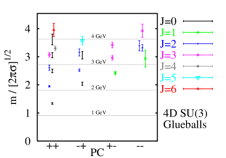
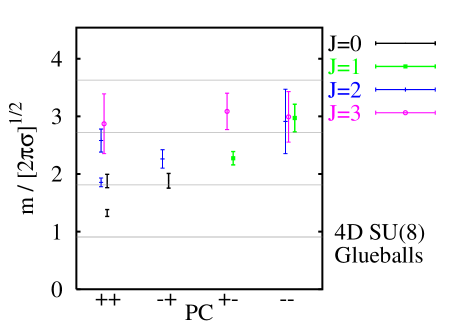
Figure 6: The continuum spectrum of glueballs in the 4D pure $SU(3)$ and $SU(8)$ gauge theories. The physical scale was set using $\sqrt{\sigma}=440$MeV.

6 Conclusions

Using novel lattice techniques, we have calculated the masses of higher spin glueballs in the continuum limit of the SU(3) gauge theory. In the physically interesting case of 3+1 dimensions we find a leading $PC=++$ glueball trajectory

$$\alpha_{P}(t)=0.93(24)+0.25(2)t$$ (15)

(in GeV units, using a conventional value of the string tension, $\surd\sigma\simeq 420\,\mathrm{MeV}$, and assuming linearity) which is entirely consistent with the phenomenological Pomeron. The sub-leading trajectory has a larger slope and eventually ‘crosses’ the Pomeron. We argue that such a rich Regge structure for glueballs occurs naturally within string models: while quarkonia arise only from open strings (of fundamental flux joining two quarks), glueballs can arise not only from open strings (of adjoint flux, joining two gluons), but also from closed strings (closed loops of fundamental flux). The latter obtains its angular momentum both from two kinds of ‘phonons’ running around the perimeter and from rotations of the whole loop around a diameter. Asymptotic calculations suggest an interesting structure of non-parallel as well as parallel trajectories. Whether this might bear upon the existence of the ‘hard’ Pomeron is an interesting question.

To try and identify the dynamical content of the different trajctories, we also calculated states with other $P$ and $C$. We then argued that the states on the Pomeron are given by a rotating open string while the sub-leading trajectory has the characteristics of a closed string whose spin comes from phonons running around in the plane of the loop.

In contrast to this, we find that in 2+1 dimensions the intercept of the leading trajectory is negative so that the Pomeron in that case does not contribute significantly to scattering at high energies. Here again we find evidence that the leading trajectory is an open string while the non-leading one is a closed string. In this case we have enough accurately calculated glueball states along the leading trajectory to demonstrate its approximate linearity.

Of course it is only at $N=\infty$ that one can expect Regge trajectories to be exactly linear and glueballs to define the physical Pomeron. We showed through a calculation of the SU(8) glueball spectrum that SU(3) is indeed close to $N=\infty$ for the low-lying glueball spectrum with a single striking exception that we interpreted as the first signal of the new closed $k$-string states one expects to appear at higher $N$.

Finally, we briefly comment upon high energy scattering. As $N\to\infty$ the usual counting arguments tell us that scattering amplitudes vanish. So at large $N$ we expect the partial waves to be far from the unitarity limit, i.e. little shadowing, and so the additive quark counting rule for Pomeron coupling to hadrons is natural. The experimentally observed additive quark rule thus constitutes one more indication that QCD is ‘close’ to SU($\infty$). If the Pomeron intercept is higher than unity, then at high enough energy this will break down, and shadowing will become important so that the cross-section can satisfy the Froissart bound.

In a world with only bottom quarks, the Froissart bound $\sigma_{\rm tot}\leq\frac{\pi}{m_{G}^{2}}\log^{2}\left(\frac{s}{s_{0}}\right)$ is stronger by two orders of magnitude. Our glueball data strongly suggests that high-energy cross-sections are approximately constant in the quenched world and that its ’pomeron’ trajectory has properties very similar to the real-world pomeron. It provides a (partial) justification for perturbative analyses that are based on the gluon field only and are meant to describe the real world. But it is clear that in such frameworks, unitarisation should be enforced with respect to the gluonic Froissart bound.

We can also turn the argument around. Experimentally, the high-energy $pp$ cross-section lies only slightly under the Froissart bound of gluodynamics for $m_{G}\simeq 1.6$GeV. If the $pp$ cross-section is found to exceed it at the Large Hadron Collider, then it will definitely be necessary to include the effects of light quarks in the description of the hadronic wave-functions at that energy.

References

- [1] A. B. Kaidalov, hep-ph/0103011.
- [2] J.R. Forshaw, D.A. Ross, “Quantum Chromodynamics and the Pomeron”, Cambridge Lecture Notes in Physics, CUP 1997. S. Donnachie, G. Dosch, P. Landshoff, O. Nachtmann, “Pomeron Physics and QCD”, CUP 2004.
- [3] P.V. Landshoff, hep-ph/0108156.
- [4] H. B. Meyer and M. J. Teper, Nucl. Phys. B 658 (2003) 113 [hep-lat/0212026].
- [5] H. B. Meyer and M. J. Teper, Nucl. Phys. B 668 (2003) 111 [hep-lat/0306019].
- [6] H. B. Meyer, D. Phil. thesis, Oxford University, in preparation; H. B. Meyer, M. Teper, in preparation.
- [7] H. B. Meyer, JHEP 0301 (2003) 048 [hep-lat/0209145].
- [8] H. B. Meyer, JHEP 0401 (2004) 030 [hep-lat/0312034].
- [9] L.Pando Zayas, J. Sonnenschein and D. Vaman, hep-th/0311190.
- [10] C. Ewerz, hep-ph/0306137.
- [11] B. Lucini and M. Teper, JHEP 0106 (2001) 050 [hep-lat/0103027].
- [12] D. Perkins, “Introduction to High Energy Physics” Addison-Wesley, 1972.
- [13] S. Deldar, Phys. Rev. D62, 034509 (2000) [hep-lat/9911008]; G. S. Bali, Phys. Rev. D62, 114503 (2000) [hep-lat/0006022].
- [14] N. Isgur and J. Paton, Phys. Rev. D 31 (1985) 2910.
- [15] A. J. Niemi, (2003), hep-th/0312133.
- [16] M. J. Teper, Phys. Rev. D 59 (1999) 014512 [hep-lat/9804008].
- [17] B. Lucini, M. Teper and U. Wenger, JHEP 0406 (2004) 012 [hep-lat/0404008].
- [18] B. Lucini and M. Teper, Phys. Rev. D64, 105019 (2001) [hep-lat/0107007].
- [19] K. Hagiwara et al. [Particle Data Group Collaboration], Phys. Rev. D 66 (2002) 010001.