Abstract

We determine the weak mixing angle in the $\overline{\rm MS}$-scheme, $\sin^{2}\hat{\theta}_{W}(\mu)$, at energy scales $\mu$ relevant for present and future low energy electroweak measurements. We relate the renormalization group evolution of $\sin^{2}\hat{\theta}_{W}(\mu)$ to the corresponding evolution of ${\hat{\alpha}}(\mu)$ and include higher-order terms in $\alpha_{s}$ and $\alpha$ that had not been treated in previous analyses. We also up-date the analysis of non-perturbative, hadronic contributions and argue that the associated uncertainty is small compared to anticipated experimental errors. The resulting value of the low-energy $\overline{\rm MS}$ weak mixing angle is $\sin^{2}\hat{\theta}_{W}(0)=0.23867\pm 0.00016$.

1 Introduction

The weak mixing angle is one of the fundamental parameters of the electroweak Standard Model (SM). It can be defined through the relation,

$$\sin^{2}\theta_{W}={{g^{\prime}}^{2}\over g^{2}+{g^{\prime}}^{2}},$$ (1)

where $g$ and $g^{\prime}$ are the $SU(2)_{L}$ and $U(1)_{Y}$ gauge couplings, respectively. Its value is not predicted and needs to be extracted from parity violating neutral current experiments, where by far the most precise results were obtained at the $Z$ factories LEP 1 and SLC. Electroweak symmetry breaking provides masses for the $W$ and $Z$ bosons proportional to their gauge interactions. Therefore, one has the additional relation,

$$\sin^{2}\theta_{W}=1-{M_{W}^{2}\over M_{Z}^{2}},$$ (2)

and the gauge boson mass ratio provides independent precise information on $\sin^{2}\theta_{W}$. Extracting the fine structure constant,

$$\alpha={e^{2}\over 4\pi}={g^{2}\sin^{2}\theta_{W}\over 4\pi},$$ (3)

from the quantum Hall effect or the anomalous magnetic moment of the electron, then fixes both gauge couplings. Eqs. (1) and (3) are valid at the tree level and modified by radiative corrections. As a result, the precise numerical value of $\sin^{2}\theta_{W}$ depends on the renormalization scheme and scale chosen. For example, the on-shell renormalization scheme promotes Eq. (2) to a definition of $\sin^{2}\theta_{W}\equiv\sin^{2}\theta_{W}^{\rm\;on-shell}$ to all orders in perturbation theory. This definition has the advantage of being directly related to a physical observable — but only to one-loop order. Since the gauge bosons are unstable particles their masses become ambiguous starting at two-loop precision.

As an alternative, one can define flavor-dependent “effective” mixing angles appearing in the $Z$ vector coupling,

$$v_{f}=T_{f}-2Q_{f}\sin^{2}\theta_{f}^{\rm\;eff},$$ (4)

where $Q_{f}$ and $T_{f}$ are the fermion charge and third component of isospin, respectively. Gauge boson self-energy and $Zf{\bar{f}}$-vertex corrections are absorbed into scheme dependent form factors, $\rho_{f}$ and $\kappa_{f}$ that are equal to unity at tree-level. The $\rho_{f}$ are corrections to the overall coupling strengths and the $\kappa_{f}$ are defined by,

$$\sin^{2}\theta_{f}^{\rm\;eff}\equiv\kappa_{f}\sin^{2}\theta_{W}^{\rm\;on-shell}\equiv\hat{\kappa}_{f}\sin^{2}\hat{\theta}_{W}(M_{Z}),$$ (5)

where the caret marks quantities in the modified minimal subtraction ($\overline{\rm MS}$) scheme [?–?]. This effective $\sin^{2}\theta_{f}^{\rm\;eff}$ is a useful definition as long as electroweak box contributions can be neglected; since these do not resonate this condition is clearly satisfied at LEP 1 and SLC. However, with the greater precision that could be achieved with the GigaZ option of TESLA, such boxes could become non-negligible. Thus, it is not easy to construct a definition that can be equated to a physical observable to all orders. Neither is this of practical relevance: as long as it is well-defined, $\sin^{2}\theta_{W}$ can be looked upon as a mere bookkeeping device and means to compare various experimental results.

What is of practical importance, however, is the numerical value of the mixing angle used in computing a given observable in a specified renormalization scheme. Generally speaking, one expects a one-loop radiatively corrected result to be valid up to small corrections of ${\cal O}({\alpha^{2}\over\pi^{2}\sin^{4}\theta_{W}})\sim 10^{-4}$. On the other hand, for leptons we have,

$$(\kappa_{\ell}-1)^{2}\approx 1.5\times 10^{-3},$$ (6)

which is not much smaller than a typical one-loop contribution. The reason is that $\kappa_{\ell}$ contains top-quark mass enhancements factors, $m_{t}^{2}/M_{W}^{2}$, that spoil the expected behavior of the perturbation series. Fortunately, such enhancement factors can be avoided by a judicious choice of definition of the weak mixing angle (or renormalization scheme), rendering the truncation error small. The $\overline{\rm MS}$-definition considered in this article has this property, except that small $\ln m_{t}^{2}/M_{W}^{2}$ corrections cannot be decoupled simultaneously from all observables [5, 6].

For processes off the $Z$-pole, enhancement factors of similar magnitude as those entering Eq. (6) can arise from large logarithms $\ln M_{Z}^{2}/m_{f}^{2}$, where $m_{f}$ is some fermion mass. These can occur even within a specifically chosen renormalization scheme. Typically, such logarithms are artifacts of using a value for $\sin^{2}\theta_{W}$ obtained at the $Z$ scale (where as noted above, it is measured very precisely) in theoretical expressions for very low (or high) energy observables. In some renormalization schemes, the weak mixing angle depends explicitly on a renormalization scale parameter, which could be the t’Hooft scale, $\mu$, appearing in dimensional regularization, or the momentum transfer $q^{2}$. For others there is no explicit scale parameter, and the scale dependence is of indirect nature. In either case, the aforementioned logarithms are a potential hazard and should be avoided or re-summed if possible.

The main goal of this paper is to present an analysis of the weak mixing angle in the $\overline{\rm MS}$-scheme, $\sin^{2}\hat{\theta}_{W}(0)$, relevant for observables measured at (almost) vanishing momentum transfer. These observables include the nuclear weak charge obtained in the well-known cesium atomic parity violation measurement performed by the Boulder group [7]; the parity violating Møller asymmetry at SLAC [8]; and the up-coming measurement of the weak charge of the proton at Jefferson Lab [9]. Precision measurements of the parity violating deep inelastic $eD$ asymmetry have also been discussed as future possibilities for Jefferson Lab, as has a more precise measurement of the Møller asymmetry. The value of $\sin^{2}\hat{\theta}_{W}(0)$ is particularly relevant for the interpretation of the parity violation experiments, since the vector coupling of the $Z$ n Eq. (4) to electrons and protons is proportional to $1-4\sin^{2}\theta_{W}(q^{2})^{\rm eff}_{f}\sim 0.1$ and is, therefore, highly sensitive to the value of the effective weak mixing angle. Indeed, as noted in Refs. [10, 11], one-loop contributions to $\sin^{2}\theta_{W}(0)^{\rm eff}_{f}$ reduce the magnitude of the Møller asymmetry by roughly 40% from its tree-level value, an effect generated by the large logarithms discussed above. Moreover, the presence of these large logarithms in $\sin^{2}\theta_{W}(0)^{\rm eff}_{f}$ is universal to all low energy neutral current observables, though their net effect may be masked by other enhanced radiative corrections. Consequently, one would like to sum these universally enhanced contributions to all orders. Here, we do so using the renormalization group evolution for $\sin^{2}\hat{\theta}_{W}(\mu)$ in the $\overline{\rm MS}$-scheme.

The $\overline{\rm MS}$-definition of the weak mixing angle is, of course, not unique, and one may choose an alternate scheme in which to compute radiative corrections to electroweak observables. Nevertheless, the $\overline{\rm MS}$-scheme offers several advantages that motivate our adoption of it here. In particular, the $\overline{\rm MS}$-definition of $\sin^{2}\hat{\theta}_{W}(\mu)$ follows closely the coupling-based definition in Eq. (1) with a well-defined subtraction of singular terms arising in dimensional regularization, giving rise to expressions with a logarithmic $\mu$-dependence. This dependence is governed by a renormalization group equation (RGE), and choosing $\mu$ equal to the momentum transfer of the process under consideration will in general avoid spurious logarithms. As we discuss below, the evolution of $\sin^{2}\hat{\theta}_{W}(\mu)$ can be related in a straightforward way to that of ${\hat{\alpha}}(\mu)$, the QED coupling in the $\overline{\rm MS}$-scheme that has been thoroughly studied elsewhere. Doing so allows us to draw upon known results for the QED $\beta$-function and – in conjunction with suitable matching conditions – to improve the precision of the Standard Model predictions for low-energy observables by incorporating various higher order effects. Indeed, although the one-loop RGE for $\sin^{2}\hat{\theta}_{W}(\mu)$ has been well-studied by others, one emphasis of the present work is the inclusion of higher order QED and perturbative QCD contributions in a systematic way. We discuss the RGE in Sections 2 and 3, and matching conditions in Section 4.

A major complication arises when the contribution of the light quark flavors is considered for $\mu$ of order a hadronic scale, $\Lambda$, or smaller. In this regime, QCD corrections to the RGE ($\beta$-function) cannot be obtained using perturbative methods. An analogous problem is well-known to arise for $\hat{\alpha}(\mu)$ when its value is desired at scales similar to or greater than $\Lambda$. We address this problem in Sections 5 and 6, as well as two appendices. We argue that the corresponding theoretical uncertainty is well below the anticipated experimental errors and provide a new estimate of this uncertainty that is substantially smaller in magnitude than the previously-quoted one [15]. Non-logarithmic contributions and some more formal aspects are discussed in Section 7 while numerical results and a plot of $\sin^{2}\hat{\theta}_{W}(\mu)$ for $\mu=\sqrt{|q^{2}|}$ – along with conclusions – are presented in Section 8. We note there our results may also be applied to the recent studies of deep-inelastic neutrino-nucleus scattering carried out by the NuTeV Collaboration [16].

2 Leading order RGE analysis

The quantity $\sin^{2}\hat{\theta}_{W}(0)$ is related to $\hat{s}^{2}_{Z}\equiv\sin^{2}\hat{\theta}_{W}(M_{Z})$ by,

$$\sin^{2}\hat{\theta}_{W}(0)\equiv\hat{\kappa}(0)\sin^{2}\hat{\theta}_{W}(M_{Z})\equiv[1+\Delta\hat{\kappa}(0)]\hat{s}^{2}_{Z},$$ (7)

where $\Delta\hat{\kappa}(0)$ is a universal (flavor-independent) radiative correction. In this Section we are interested in logarithmic contributions to $\hat{\kappa}(0)$ of the form,

$${\hat{\alpha}\over\pi\sin^{2}\hat{\theta}_{W}}\ln{M_{Z}^{2}\over m_{i}^{2}},$$

and in particular in the scale that should be used in $\hat{\alpha}$ and $\sin^{2}\hat{\theta}_{W}$, appropriate for re-summing the leading, large logarithms to all orders. These logarithms arise from scale dependent self-energy mixing diagrams where one external leg is a photon and the other one is a $Z$-boson. Thus, $v_{f}$ acquires a compensating scale dependence,

$$\hat{v}_{f}\left(\sqrt{\mu^{2}+\Delta\mu^{2}}\right)=\hat{v}_{f}(\mu)+{\hat{\alpha}(\mu)\over 24\pi}Q_{f}\sum\limits_{i}[N^{c}_{i}\gamma_{i}v_{i}(\mu)Q_{i}]\ln{\mu^{2}+\Delta\mu^{2}\over\mu^{2}},$$ (8)

where $N^{c}_{q}=N_{C}=3$ (for quarks) and $N^{c}_{\ell}=1$ (for leptons) is the color factor. We have written the sum in general form to also allow chiral fermions and bosonic degrees of freedom (to put the $W^{\pm}$ and Higgs ghosts on the same footing as the fermions and to facilitate the discussion in Section 7), where the spin dependent factors $\gamma_{i}$ are shown in Table 1.

field	$\gamma_{i}$
real scalar	1
complex scalar	2
chiral fermion	4
Majorana fermion	4
Dirac fermion	8
massless gauge boson	$-22$

Table 1: Weight factors $\gamma_{i}$ entering the leading RGE coefficients for the weak mixing angle.

With these conventions, the factor of 1/24 also appears in the lowest order QED $\beta$-function coefficient,

$$\mu^{2}{d\hat{\alpha}\over d\mu^{2}}={\hat{\alpha}^{2}\over 24\pi}\sum\limits_{i}N^{c}_{i}\gamma_{i}Q_{i}^{2}.$$ (9)

This implies the RGE,

$$\mu^{2}{d\hat{v}_{f}\over d\mu^{2}}={\hat{\alpha}\over 24\pi}Q_{f}\sum\limits_{i}N^{c}_{i}\gamma_{i}\hat{v}_{i}Q_{i},$$ (10)

or in terms of the variable $\hat{X}=\sum_{i}N^{c}_{i}\gamma_{i}\hat{v}_{i}Q_{i}$,

$${d\hat{X}\over\hat{X}}={\hat{\alpha}\over 24\pi}{d\mu^{2}\over\mu^{2}}\sum\limits_{i}N^{c}_{i}\gamma_{i}Q_{i}^{2}={d\hat{\alpha}\over\hat{\alpha}},$$ (11)

where in the second equality we used Eq. (9). This is solved by,

$$\sin^{2}\hat{\theta}_{W}(\mu)={\hat{\alpha}(\mu)\over\hat{\alpha}(\mu_{0})}\sin^{2}\hat{\theta}_{W}(\mu_{0})+{\sum_{i}N^{c}_{i}\gamma_{i}Q_{i}T_{i}\over\sum_{i}N^{c}_{i}\gamma_{i}Q_{i}^{2}}\left[1-{\hat{\alpha}(\mu)\over\hat{\alpha}(\mu_{0})}\right],$$ (12)

or using the explicit solution to the one-loop RGE in Eq. (9) we obtain the simpler form,

$$\sin^{2}\hat{\theta}_{W}(\mu)=\sin^{2}\hat{\theta}_{W}(\mu_{0})\left[1+{\hat{\alpha}(\mu)\over 24\pi\sin^{2}\hat{\theta}_{W}(\mu_{0})}\sum\limits_{i}N_{i}^{c}\gamma_{i}Q_{i}[T_{i}-Q_{i}\sin^{2}\hat{\theta}_{W}(\mu_{0})]\ln{\mu_{0}^{2}\over\mu^{2}}\right].$$ (13)

The result in Eq. (13) re-sums all logarithms of ${\cal O}(\alpha^{n}\ln^{n}{\mu_{0}\over\mu})$ provided there is no particle threshold between $\mu$ and $\mu_{0}$. To avoid reintroduction of spurious logarithms this solution must be applied successively from one particle threshold to the next. Crossing a threshold from above, the corresponding particle is integrated out, and one continues with an effective field theory without this particle. In contrast, changing from one effective field theory to another far away from the physical mass of the particle would not formally affect the truncated one-loop result, but it would spoil its re-summation.

Eq. (13) applied to $\Delta\kappa(0)$ can be brought into the well-known form [14],

$$\Delta\kappa(0)={\alpha\over\pi\hat{s}^{2}_{Z}}\left[{1\over 6}\sum\limits_{f}N_{f}^{c}Q_{f}(T_{f}-2Q_{f}\hat{s}^{2}_{Z})\ln{M_{Z}^{2}\over m_{f}^{2}}-\left({43\over 24}-{7\over 4}\hat{s}^{2}_{Z}\right)\ln{M_{Z}^{2}\over M_{W}^{2}}\right],$$ (14)

where the sum is over all SM Dirac fermions excluding the top quark. The last term is the $W^{\pm}$ contribution with its coefficient obtainable from Table 1 when a pair of massless gauge bosons ($T_{i}=\pm 1$) is combined with a complex scalar Goldstone degree of freedom ($T_{i}=\pm 1/2$).

3 Higher order RGE analysis

In this Section we will generalize the leading order analysis and re-sum next-to-leading (NL) logarithms of ${\cal O}(\alpha^{n+1}\ln^{n}{\mu_{0}\over\mu})$ and ${\cal O}(\alpha\alpha_{s}^{n}\ln^{n}{\mu_{0}\over\mu})$, as well as the NNL logarithms of ${\cal O}(\alpha\alpha_{s}^{n+1}\ln^{n}{\mu_{0}\over\mu})$, and the NNNL logarithms of ${\cal O}(\alpha\alpha_{s}^{n+2}\ln^{n}{\mu_{0}\over\mu})$. The leading order RGE (11) supplemented by terms of ${\cal O}(\alpha^{2})$, ${\cal O}(\alpha\alpha_{s})$, ${\cal O}(\alpha\alpha_{s}^{2})$, and ${\cal O}(\alpha\alpha_{s}^{3})$ reads,

$$\mu^{2}{d\hat{v}_{f}\over d\mu^{2}}={\hat{\alpha}\over 24\pi}Q_{f}\left[\sum\limits_{i}K_{i}\gamma_{i}\hat{v}_{i}Q_{i}+12\sigma\left(\sum\limits_{q}\hat{v}_{q}\right)\left(\sum\limits_{q}Q_{q}\right)\right],$$ (15)

where in the case of quarks ($n_{q}$ is the effective number of quarks),

$$K_{i}=N_{i}^{c}\left\{1+{3\over 4}Q_{i}^{2}{\hat{\alpha}\over\pi}+{\hat{\alpha}_{s}\over\pi}+{\hat{\alpha}_{s}^{2}\over\pi^{2}}\left({125\over 48}-{11\over 72}n_{q}\right)+\right.$$ (16)

$$\left.{\hat{\alpha}_{s}^{3}\over\pi^{3}}\left[{10487\over 1728}+{55\over 18}\zeta(3)-\left({707\over 864}+{55\over 54}\zeta(3)\right)n_{q}-{77\over 3888}n_{q}^{2}\right]\right\},$$

contains QED and QCD corrections [?–?] to the lowest order (non-singlet) vacuum polarization diagrams. For leptons only the term involving $\hat{\alpha}$ is kept, while for bosons we restrict ourselves to the lowest order $\beta$-function, i.e. $K_{W^{\pm}}=1$. The second sum in Eq. (15) is over Dirac quark fields, and

$$\sigma={\hat{\alpha}_{s}^{3}\over\pi^{3}}\left[{55\over 216}-{5\over 9}\zeta(3)\right]+{\cal O}(\hat{\alpha}_{s}^{4}),$$ (17)

parametrizes the QCD singlet contribution. In a singlet (QCD annihilation) diagram two independent fermion loops are attached to the $\gamma$ and $Z$ and connected to each other by gluons or photons. Due to Furry’s theorem, connections containing a photon first arise at ${\cal O}(\alpha^{2}\alpha_{s}^{2})$ and can safely be neglected. Defining $\hat{s}^{2}=\sin^{2}\hat{\theta}_{W}(\mu)$ we rewrite Eq. (15),

$$\mu^{2}{d\hat{s}^{2}\over d\mu^{2}}={\hat{\alpha}\over\pi}\left[{1\over 24}\sum\limits_{i}K_{i}\gamma_{i}(Q_{i}^{2}\hat{s}^{2}-T_{i}Q_{i})+\sigma\hat{s}^{2}\left(\sum\limits_{q}Q_{q}\right)^{2}-{\sigma\over 2}\left(\sum\limits_{q}T_{q}\right)\left(\sum\limits_{q}Q_{q}\right)\right].$$ (18)

Similarly, the RGE for $\hat{\alpha}$ including higher orders reads,

$$\mu^{2}{d\hat{\alpha}\over d\mu^{2}}={\hat{\alpha}^{2}\over\pi}\left[{1\over 24}\sum\limits_{i}K_{i}\gamma_{i}Q_{i}^{2}+\sigma\left(\sum\limits_{q}Q_{q}\right)^{2}\right],$$ (19)

and we obtain,

$$\mu^{2}{d\over d\mu^{2}}\left({\hat{s}^{2}\over\hat{\alpha}}\right)=-{1\over 24\pi}\sum_{i}K_{i}\gamma_{i}T_{i}Q_{i}-{\sigma\over 2\pi}\left(\sum\limits_{q}T_{q}\right)\left(\sum\limits_{q}Q_{q}\right).$$ (20)

To facilitate the integration and to relate hadronic contributions as far as possible to the ones in $\hat{\alpha}$, we use Eq. (19) again and eliminate all $\hat{\alpha}_{s}$ dependent terms in Eq. (16). With the coefficients,

$$\lambda_{1}={\sum_{q}T_{q}Q_{q}\over 2\sum_{q}Q^{2}_{q}},\hskip 50.0pt\lambda_{2}={1\over 8}\sum\limits_{i\neq q}\gamma_{i}(\lambda_{1}Q_{i}^{2}-T_{i}Q_{i})={1\over 8}\sum\limits_{i}N_{i}^{c}\gamma_{i}(\lambda_{1}Q_{i}^{2}-T_{i}Q_{i}),$$ (21)

and,

$$\lambda_{3}={\sum_{i}N_{i}^{c}\gamma_{i}[\lambda_{1}Q_{i}^{4}-T_{i}Q_{i}^{3}]\over\sum_{i}N^{c}_{i}\gamma_{i}Q^{2}_{i}},\hskip 40.0pt\lambda_{4}=\left[\lambda_{1}\left(\sum\limits_{q}Q_{q}\right)^{2}-{1\over 2}\left(\sum\limits_{q}T_{q}\right)\left(\sum\limits_{q}Q_{q}\right)\right],$$ (22)

shown in Table 2 this can be brought into the form,

energy range	$\lambda_{1}$	$\lambda_{2}$	$\lambda_{3}$	$\lambda_{4}$
$\bar{m}_{t}\leq\mu\hskip 36.0pt$	9/20	289/80	14/55	9/20
$M_{W}\leq\mu<\bar{m}_{t}\hskip 6.0pt$	21/44	625/176	6/11	3/22
$\bar{m}_{b}\leq\mu<M_{W}$	21/44	15/22	51/440	3/22
$m_{\tau}\leq\mu<\bar{m}_{b}\hskip 6.0pt$	9/20	3/5	2/19	1/5
$\bar{m}_{c}\leq\mu<m_{\tau}\hskip 5.0pt$	9/20	2/5	7/80	1/5
$\bar{m}_{s}\leq\mu<\bar{m}_{c}\hskip 5.0pt$	1/2	1/2	5/36	0
$\bar{m}_{d}\leq\mu<\bar{m}_{s}\hskip 5.0pt$	9/20	2/5	13/110	1/20
$\bar{m}_{u}\leq\mu<\bar{m}_{d}\hskip 5.0pt$	3/8	1/4	3/40	0
$m_{\mu}\leq\mu<\bar{m}_{u}\hskip 5.0pt$	1/4	0	0	0
$m_{e}\leq\mu<m_{\mu}\hskip 5.0pt$	1/4	0	0	0
$\mu<m_{e}\hskip 6.0pt$	0	0	0	0

Table 2: Coefficients entering the higher order RGE for the weak mixing angle. For the definition of quark threshold masses, $\bar{m}_{q}$, see Section 5. Below hadronic scales $\lambda_{1}$ is not defined through Eq. (21) and can be chosen arbitrarily; we chose the value, $\lambda_{1}=1/4$, to obtain $\lambda_{2}=\lambda_{3}=0$.

$$\mu^{2}{d\over d\mu^{2}}\left({\hat{s}^{2}-\lambda_{1}\over\hat{\alpha}}-{3\lambda_{3}\over 4\pi}\ln\hat{\alpha}+{\tilde{\sigma}\over\pi}\right)={\lambda_{2}\over 3\pi}.$$ (23)

For the last term on the left hand side we have used the lowest order QCD $\beta$-function coefficient and have defined

$$\tilde{\sigma}(\mu)=\lambda_{4}{\hat{\alpha}_{s}^{2}(\mu)\over\pi^{2}}{5\over 36}{11-24\zeta(3)\over 33-2n_{q}}+{\cal O}(\hat{\alpha}_{s}^{3}).$$ (24)

The solution to Eq. (23) is given by,

$$\hat{s}^{2}(\mu)={\hat{\alpha}(\mu)\over\hat{\alpha}(\mu_{0})}\hat{s}^{2}(\mu_{0})+\lambda_{1}\left[1-{\hat{\alpha}(\mu)\over\hat{\alpha}(\mu_{0})}\right]+{\hat{\alpha}(\mu)\over\pi}\left[{\lambda_{2}\over 3}\ln{\mu^{2}\over\mu_{0}^{2}}+{3\lambda_{3}\over 4}\ln{\hat{\alpha}(\mu)\over\hat{\alpha}(\mu_{0})}+\tilde{\sigma}(\mu_{0})-\tilde{\sigma}(\mu)\right].$$ (25)

Hadronic uncertainties are induced through $\hat{\alpha}(\mu)$, through the relative values of the light quark threshold masses, $\bar{m}_{u}$, $\bar{m}_{d}$, and $\bar{m}_{s}$ (these are needed as they determine the change of the coefficients $\lambda_{i}$ according to Table 2), and through the singlet contribution proportional to $\tilde{\sigma}(\mu_{0})-\tilde{\sigma}(\mu)$.

4 Matching conditions

At the threshold of fermion $f$ we find,

$$\sin^{2}\hat{\theta}_{W}(m_{i})^{-}={\hat{\alpha}(m_{i})^{-}\over\hat{\alpha}(m_{i})^{+}}\sin^{2}\hat{\theta}_{W}(m_{i})^{+}+{Q_{i}T_{i}\over 2Q_{i}^{2}}\left[1-{\hat{\alpha}(m_{i})^{-}\over\hat{\alpha}(m_{i})^{+}}\right],$$ (26)

where the plus (minus) superscript denote the effective theory including (excluding) fermion $f$. While the one and two-loop $\beta$-function coefficients are well-known to be renormalization scheme independent, the matching conditions are renormalization scheme and even regularization scheme dependent. The $\overline{\rm MS}$-scheme is defined by dimensional regularization which generates no ${\cal O}(\alpha)$ matching terms for scalars; with the usual additional requirement that the Clifford algebra is kept in four dimensions the same holds for spin-1/2 fermions. We include the RGE matching conditions for $\hat{\alpha}$ at the threshold for fermion $f$ at the orders $\alpha^{2}$, $\alpha\alpha_{s}$, and $\alpha\alpha_{s}^{2}$ [20, 21],

$${1\over\hat{\alpha}^{+}(m_{f})}={1\over\hat{\alpha}^{-}(m_{f})}-{Q_{f}^{2}\over\pi}\left\{{15\over 16}N^{c}_{f}Q_{f}^{2}{\hat{\alpha}(m_{f})\over\pi}+\right.$$ (27)

$$\left.{(N^{c}_{f}-1)\over 2}{\hat{\alpha}_{s}(m_{f})\over\pi}\left[{13\over 12}+{\hat{\alpha}_{s}(m_{f})\over\pi}\left({655\over 144}\zeta(3)-{3847\over 864}+{361\over 1296}n_{q}+{295\over 1296}{\sum_{q\neq f}Q_{q}^{2}\over Q_{f}^{2}}\right)\right]\right\}.$$

Here, $n_{q}$ is the number of quarks including the threshold quark $f$. Eq. (26) will then induce the corresponding matching contributions to the weak mixing angle.

In contrast to fermions and scalars, gauge bosons induce an ${\cal O}(\alpha)$ threshold shift [22],

$${1\over\alpha_{i}^{+}}={1\over\alpha_{i}^{-}}+{C(R)\over 12\pi},$$ (28)

where $C(R)$ is the quadratic Casimir of the (in general reducible) gauge boson representation, normalized such that, e.g., $C({\rm adjoint\/}[SU(N)])=N$. Thus, integrating out the $W^{\pm}$ bosons induces a shift in the electromagnetic coupling,

$${1\over\hat{\alpha}(M_{W})^{+}}={1\over\hat{\alpha}(M_{W})^{-}}+{1\over 6\pi},$$ (29)

and (generalizing Eq. (26) appropriately) in the weak mixing angle,

$$\sin^{2}\hat{\theta}_{W}(M_{W})^{+}=1-{\hat{\alpha}(M_{W})^{+}\over\hat{\alpha}(M_{W})^{-}}\cos^{2}\hat{\theta}_{W}(M_{W})^{-}.$$ (30)

5 Hadronic contribution

The ambiguity in the values of the three light quark masses plus the singlet contribution to Eq. (25) introduce four sources of hadronic uncertainties in $\sin^{2}\hat{\theta}_{W}(0)$. This problem is familiar from the evaluation of $\alpha(M_{Z})$, where it can be addressed by relating it via a dispersion relation to $e^{+}e^{-}\to$ hadrons cross section data, or (using in addition isospin symmetry) to $\tau$ decay spectral functions. The same strategy could in principle be applied here, except that the experimental information would have to be separated in charge 2/3 ($u$) vs. charge $-1/3$ ($d$ and $s$) quarks, or assuming isospin symmetry, in $s$ vs. the first generation quarks. This is a difficult task: e.g., a $K^{\pm}$ final state in $e^{+}e^{-}$ annihilation can be produced directly through an $\bar{s}\gamma_{\mu}s$ current or by splitting of a gluon radiated off a quark originating from a $\bar{u}\gamma_{\mu}u+\bar{d}\gamma_{\mu}d$ (isoscalar) current. It would be even more difficult to isolate the singlet contribution. As for $\tau^{-}$ decays, the relatively large $m_{s}$ induces a sizable axial-vector contribution to final states with strangeness, $S=-1$. At least presently, it cannot be cleanly separated from the vector contribution which is the relevant one for the problem at hand. We will therefore follow a different strategy and show that the four uncertainties can be traded for the uncertainties associated with (i) the value of ${\hat{\alpha}}(M_{Z})$, which we denote $\delta_{\alpha}\sin^{2}\hat{\theta}_{W}(0)$, with (ii) the separation of strange and first generation quark effects, indicated by $\delta_{s}\sin^{2}\hat{\theta}_{W}(0)$, with (iii) deviations from isospin symmetry, $\delta_{\rm CVC}\sin^{2}\hat{\theta}_{W}(0)$, and with (iv) Zweig (OZI) rule deviations, $\delta_{\rm OZI}\sin^{2}\hat{\theta}_{W}(0)$.

As discussed in Section 3, the contributions of leptons and heavy quarks can be computed unambiguously in perturbation theory. Indeed, using QCD $\overline{\rm MS}$ masses, $\hat{m}_{q}(\hat{m}_{q})$, will provide a small truncation error, $\delta_{\rm PQCD}\sin^{2}\hat{\theta}_{W}(0)$, in the perturbative expansion (cf. the small matching coefficients in Eq. (27)). Moreover, the numerical values of $\hat{m}_{q}(\hat{m}_{q})$ can be determined to sufficient precision that is not limited by uncertainties of the order of hadronic scales. Therefore, we compute first $\sin^{2}\hat{\theta}_{W}(\bar{\mu})$ from $\sin^{2}\hat{\theta}_{W}(M_{Z})$ (which can be taken from $Z$ pole experiments), where $\bar{\mu}$ corresponds to a scale where the heavy flavors ($b$, $c$, and $\tau$) are integrated out, and at which we still have sufficient confidence in the convergence of perturbative QCD (i.e., of order 1 GeV).

We constrain the contributions of light quarks to $\sin^{2}\hat{\theta}_{W}(\bar{\mu})$ phenomenologically. Our strategy is to employ the $u$, $d$, and $s$ quark contributions to $\hat{\alpha}(\bar{\mu})$, $\Delta\hat{\alpha}^{(3)}(\bar{\mu})$, as a constraint, and to find upper and lower bounds on the strange quark contribution relative to the contributions of the first generation quarks. In the following we assume isospin symmetry and a vanishing singlet contribution. Deviations from these assumptions will be addressed in Section 6.

To facilitate the discussion, we will adopt definitions of threshold quark masses, $\bar{m}_{u}$, $\bar{m}_{d}$, and $\bar{m}_{s}$, such that Eq. (25) remains valid with trivial matching conditions, $\alpha_{i}^{+}(\bar{m}_{q})=\alpha_{i}^{-}(\bar{m}_{q})$. Thus, $\bar{m}_{u}$, $\bar{m}_{d}$, and $\bar{m}_{s}$ define the ranges in Table 2. Their values can be constrained phenomenologically, but their relation to other mass definitions, such as constituent masses or current masses, cannot be written down in a perturbative sense. One combination of the three light quark threshold masses is constrained to reproduce $\hat{\alpha}(\bar{\mu})/\alpha$. If we assume isospin symmetry, $\bar{m}_{u}=\bar{m}_{d}$, and a vanishing singlet contribution, we have only one unknown parameter, say $\bar{m}_{s}$, to describe $\delta_{s}\sin^{2}\hat{\theta}_{W}(0)$. Before we use physics arguments to constrain $\bar{m}_{s}$, we compute $\bar{m}_{c}$ and $\bar{m}_{b}$ perturbatively to gauge the behavior of heavy quarks. To order $\alpha_{s}^{2}$ we have [20, 21],

$$\ln{\mu^{2}\over\hat{m}^{2}(\mu)}+{\hat{\alpha}_{s}(\mu)\over\pi}\left[{13\over 12}-\ln{\mu^{2}\over\hat{m}^{2}(\mu)}\right]+{\hat{\alpha}_{s}^{2}\over\pi^{2}}\left[{655\over 144}\zeta(3)-{3847\over 864}+n_{q}{361\over 1296}+{295\over 1296}{\sum_{q\neq f}Q_{q}^{2}\over Q_{f}^{2}}\right]=0,$$ (31)

which implies,

$$\bar{m}=\hat{m}(\hat{m})\exp\left[-{13\over 24}{\hat{\alpha}_{s}(\hat{m})\over\hat{\alpha}_{s}(\hat{m})+\pi}-{\hat{\alpha}_{s}^{2}\over 288\pi^{2}}\left(655\zeta(3)-{3847\over 6}+{361\over 9}n_{q}+{295\over 9}{\sum_{q\neq f}Q_{q}^{2}\over Q_{f}^{2}}\right)\right].$$ (32)

With the input values (obtained from a global fit to precision data), $\hat{\alpha}_{s}(M_{Z})=0.1214\pm 0.0018$, $\hat{m}_{c}(\hat{m}_{c})=1.285_{-0.047}^{+0.040}$, and $\hat{m}_{b}(\hat{m}_{b})=4.205\pm 0.031$, we find $\bar{m}_{c}=1.176$ GeV and $\bar{m}_{b}=3.995$ GeV.

The heavy $\bar{m}_{s}$ limit

To obtain a lower limit on the strange quark contribution to $\hat{\alpha}(\bar{\mu})$, we consider the case in which the strange quark is assumed to behave like a heavy quark. In this case, $\bar{m}_{s}$ would be related to $M_{\phi}$ in a similar way as $\bar{m}_{c}$ (or $\hat{m}_{c}(\hat{m}_{c})$) is related to $M_{J/\Psi}$. Defining $\xi_{q}=2\bar{m}_{q}/M_{1S}$ where $M_{1S}$ is the mass of the $1S$ $q\bar{q}$ resonance, we have that asymptotically $\xi_{q}\to 1$ for $\bar{m}_{q}\to\infty$ and $\xi_{q}\to 0$ for $\bar{m}_{q}\to 0$ (in the chiral limit the quark contribution is logarithmically divergent). Thus, for a heavy quark $\xi_{q}\sim 1$, while for a light quark $\xi_{q}\ll 1$. Also, we expect $\bar{m}_{1}<\bar{m}_{2}\Longrightarrow\xi_{1}<\xi_{2}$. As an illustration, with the numerical values of $\bar{m}_{c}$ and $\bar{m}_{b}$ from above we obtain $\xi_{c}=0.759$, $\xi_{b}=0.845$, and $\bar{m}_{s}=\xi_{s}M_{\phi}/2<\xi_{c}M_{\phi}/2=387$ MeV. As a refinement we introduce scale dependent QCD correction factors, $K_{\rm QCD}^{q}=K_{\rm QCD}(\bar{\mu},\bar{m}_{q})$, where $K_{\rm QCD}(\bar{\mu}_{1},\bar{\mu}_{2})$ denotes the average QCD correction to the QED $\beta$-functions for RGE running between scales $\bar{\mu}_{1}$ and $\bar{\mu}_{2}$. One thus expects $\bar{m}_{1}<\bar{m}_{2}\Longrightarrow K_{\rm QCD}^{1}>K_{\rm QCD}^{2}$. Since Eq. (32) applied to $m_{c}$ still shows satisfactory convergence, we can safely choose $\bar{\mu}=\bar{m}_{c}$,

$$\Delta_{s}\hat{\alpha}(\bar{m}_{c})=Q_{s}^{2}{\alpha\over\pi}K_{\rm QCD}^{s}\ln{\bar{m}_{c}^{2}\over\bar{m}_{s}^{2}}>Q_{s}^{2}{\alpha\over\pi}K_{\rm QCD}^{c}\ln{\bar{m}_{c}^{2}\over\bar{m}_{s}^{2}}>{2\alpha\over 9\pi}K_{\rm QCD}^{c}\ln{M_{J/\Psi}\over M_{\phi}}=6.9\times 10^{-4}.$$ (33)

For the numerical evaluation we have used the QCD correction in Eq. (16) applied to the effective theory with $n_{q}=3$ quarks,

$$K_{\rm QCD}^{s}>K_{\rm QCD}^{c}=1+{\hat{\alpha}_{s}(\bar{m}_{c})\over\pi}+{103\over 48}{\hat{\alpha}_{s}^{2}(\bar{m}_{c})\over\pi^{2}}+{1979\over 576}{\hat{\alpha}_{s}^{3}(\bar{m}_{c})\over\pi^{3}}=1.209,$$ (34)

and we have used $\hat{\alpha}_{s}(\bar{m}_{c})=0.469$, again corresponding to $\hat{\alpha}_{s}(M_{Z})=0.1214$.

The $SU(3)$ limit

Since $m_{s}>m_{d}\buildrel>\over{{}_{\sim}}m_{u}$ at any scale and in any reasonable definition and scheme, we conclude that the $SU(3)$ symmetric case, $\bar{m}_{u}=\bar{m}_{d}=\bar{m}_{s}$, implies an upper limit on the relative strange quark contribution to $\hat{\alpha}(\bar{\mu})$,

$$\Delta_{s}\hat{\alpha}(\bar{\mu})\leq{1\over 6}\left[\Delta_{u}\hat{\alpha}(\bar{\mu})+\Delta_{d}\hat{\alpha}(\bar{\mu})+\Delta_{s}\hat{\alpha}(\bar{\mu})\right]\equiv{1\over 6}\Delta\hat{\alpha}^{(3)}(\bar{\mu}).$$ (35)

This crude limit can be strengthened by considering the phenomenological constraint,

$${2\alpha\over\pi}\left[(Q^{2}_{u}+Q^{2}_{d})K_{\rm QCD}^{u,d}\ln{2\bar{\mu}\over\xi_{u,d}M_{\omega}}+Q^{2}_{s}K_{\rm QCD}^{s}\ln{2\bar{\mu}\over\xi_{s}M_{\phi}}\right]=\Delta\hat{\alpha}^{(3)}(\bar{\mu}),$$ (36)

and by imposing $SU(3)$ symmetry through $\xi_{u}=\xi_{d}=\xi_{s}$ and $K_{\rm QCD}^{u}=K_{\rm QCD}^{d}=K_{\rm QCD}^{s}$. This maximizes the ratio of the strange quark contribution to the one of the first generation quarks,

$${\Delta_{s}\hat{\alpha}(\bar{\mu})\over\Delta_{u+d}\hat{\alpha}(\bar{\mu})}={Q^{2}_{s}\over Q^{2}_{u}+Q^{2}_{d}}\left[1+{K^{s}_{\rm QCD}\ln{\xi_{u,d}\over\xi_{s}}-K^{s}_{\rm QCD}\ln{M_{\phi}\over M_{\omega}}-(K^{u,d}_{\rm QCD}-K^{s}_{\rm QCD})\ln{2\bar{\mu}\over\xi_{u,d}M_{\omega}}\over K^{u,d}_{\rm QCD}\ln{2\bar{\mu}\over\xi_{u,d}M_{\omega}}}\right].$$ (37)

All three corrections terms to the charge square ratio are indeed negative, and we used the second one as an improvement. In the limit $\xi_{s}\to 0$, Eq. (36) would reproduce relation (35) but now we have the constraint,

$$\xi_{s}>{2\bar{\mu}\over M_{\omega}^{5/6}M_{\phi}^{1/6}}\exp\left[-{3\pi\over 4}{\Delta\hat{\alpha}^{(3)}(\bar{\mu})\over\alpha K_{\rm QCD}^{s}}\right].$$ (38)

For the numerical evaluation we convert the contribution to the on-shell definition of $\alpha(M_{Z})$, $\Delta\alpha_{\rm had}(M_{Z})=0.00577\pm 0.00010$ [27, 28], from the energy range up to 1.8 GeV, to the $\overline{\rm MS}$-scheme,

$$\Delta\hat{\alpha}^{(3)}(\mbox{1.8~{}GeV})=\Delta\alpha_{\rm had}(M_{Z})+{2\alpha\over 3\pi}\left[{5\over 3}+\left({\hat{\alpha}_{s}\over\pi}+{\hat{\alpha}\over 4\pi}\right)\left({55\over 12}-4\zeta(3)+{2\hat{m}_{s}^{2}\over(1.8~{}{\rm GeV})^{2}}\right)+\right.$$

$$\left.{\hat{\alpha}_{s}^{2}\over\pi^{2}}\left({34525\over 864}-{9\over 4}\zeta(2)-{715\over 18}\zeta(3)+{25\over 3}\zeta(5)+F(\hat{m}_{c},\hat{m}_{b})\right)\right]=0.00831\pm 0.00010,$$

where all $\overline{\rm MS}$ running couplings and masses are to be taken at $\mu=1.8$ GeV. $F(\hat{m}_{c},\hat{m}_{b})$ contains decoupling charm and bottom mass effects [19, 29, 30]. We choose again $\bar{\mu}=\bar{m}_{c}$ and use the 4-loop RGE to obtain,

$$\Delta\hat{\alpha}^{(3)}(\bar{m}_{c})=0.00678\pm 0.00010,$$ (39)

which using the $SU(3)$ bound (38) corresponds to $\xi_{s}>0.470$ and $\bar{m}_{s}>240$ MeV. Inserting Eq. (38) into Eq. (36) in the $SU(3)$ limit yields,

$$\Delta_{s}\hat{\alpha}(\bar{m}_{c})<{\Delta\hat{\alpha}^{(3)}(\bar{m}_{c})\over 6}-{5\over 27}{\alpha\over\pi}K_{\rm QCD}^{s}\ln{M_{\phi}\over M_{\omega}}<{\Delta\hat{\alpha}^{(3)}(\bar{m}_{c})\over 6}-{5\over 27}{\alpha\over\pi}K_{\rm QCD}^{c}\ln{M_{\phi}\over M_{\omega}}=9.9\times 10^{-4}.$$ (40)

We have assumed ideal $\omega-\phi$ mixing, i.e. that the $\phi$ resonance is a pure $s\bar{s}$ state. Allowing a non-ideal mixing angle, $\epsilon=0.0548\pm 0.0024\neq 0$ (see Appendix A), shifts the masses $M_{\omega}$ and $M_{\phi}$ to be used in Eqs. (33) and (40) by less than 1 MeV and yields a negligible effect.

Implications

From Eqs. (33) and (40) we conclude for the strange quark,

$$\Delta_{s}\hat{\alpha}(\bar{m}_{c})=(8.4\pm 1.5)\times 10^{-4},\hskip 197.0pt\bar{m}_{s}=305_{+82}^{-65}\mbox{ MeV}.$$ (41)

and for the light quarks,

$$\Delta\hat{\alpha}^{(2)}(\bar{m}_{s})=\Delta\hat{\alpha}^{(3)}(\bar{m}_{c})-6\Delta_{s}\hat{\alpha}(\bar{m}_{c})=0.00172\mp 0.00090,\hskip 20.0pt\bar{m}_{d}=\bar{m}_{u}=176\pm 9\mbox{ MeV}.$$ (42)

These results can be used in the master equation (25). As an illustration, the $SU(3)$ symmetric piece is well approximated by,

$$\hat{s}^{2}(\bar{m}_{s})-\hat{s}^{2}(\bar{m}_{c})=\left[{1\over 2}-\hat{s}^{2}(\bar{m}_{c})\right]6\Delta_{s}\hat{\alpha}(\bar{m}_{c})+{2\hat{\alpha}({\bar{m}_{s}})\over 3\pi}\left[{1\over 4}-\hat{s}^{2}(\bar{m}_{c})\right]\ln{\bar{m}_{c}^{2}\over\bar{m}_{s}^{2}}\left(1+{3\hat{\alpha}({\bar{m}_{s}})\over 4\pi}\right),$$ (43)

which is obtained with the help of Table 2, and where the last term is the leptonic ($e$ and $\mu$) contribution. Similarly, the $SU(3)$ breaking piece reads,

$$\hat{s}^{2}(\bar{m}_{d})-\hat{s}^{2}(\bar{m}_{s})=\left[{9\over 20}-\hat{s}^{2}(\bar{m}_{s})\right]\Delta\hat{\alpha}^{(2)}(\bar{m}_{s})+{2\hat{\alpha}({\bar{m}_{d}})\over 3\pi}\left[{1\over 4}-\hat{s}^{2}(\bar{m}_{s})\right]\ln{\bar{m}_{s}^{2}\over\bar{m}_{d}^{2}}\left(1+{3\hat{\alpha}({\bar{m}_{d}})\over 4\pi}\right),$$ (44)

where we neglected the singlet piece involving $\bar{\sigma}$.

6 Uncertainties

From Eq. (39), as well as the sum of Eqs. (43) and (44), we can bound the uncertainty induced by $\Delta\alpha^{(3)}(\bar{m}_{c})$,

$$\delta_{\alpha}\sin^{2}\hat{\theta}_{W}(0)<\delta\Delta\alpha^{(3)}(\bar{m}_{c})\left[{1\over 2}-\hat{s}^{2}(\bar{m}_{c})\right]=\pm 3\times 10^{-5}.$$ (45)

Similarly, from the first Eq. (42) and from the comparison of the coefficients in Eqs. (43) and (44), we can estimate the uncertainty induced by $\Delta\alpha^{(2)}(\bar{m}_{s})$,

$$\delta_{s}\sin^{2}\hat{\theta}_{W}(0)\approx{1\over 20}\delta\Delta\alpha^{(2)}(\bar{m}_{s})=\pm 5\times 10^{-5}.$$ (46)

The singlet contribution

We obtained the theoretical bounds on $\bar{m}_{s}$ that are the basis for the error estimate (46) by assuming isopsin symmetry and a vanishing singlet contribution. We now relax the latter assumption and allow OZI rule [?–?] violation which leads to processes such as $\phi\to\pi^{0}\gamma$ decays and which translates on a diagrammatic level to QCD annihilation (singlet) topologies. For charm and third generation quarks singlet contributions are tiny and easily included using Eq. (17) or Eq. (24). We can then proceed with the effective theory containing only the three light quarks. Notice, that due to $Q_{u}+Q_{d}+Q_{s}=0$, there is no singlet contribution (to the $\beta$-functions of neither $\alpha$ nor $\sin^{2}\theta_{W}$) in the limit of exact $SU(3)$ symmetry (see also the sixth entry for $\lambda_{4}$ in Table 2). Moreover, allowing $SU(3)$ breaking effects — but still working in the isospin symmetric limit — will not directly affect the RGE (20) because $T_{u}+T_{d}=0$. The explicit singlet piece in Eq. (25) is an artifact of employing Eq. (19) and cancels the implicit singlet piece contained in the term proportional to $\lambda_{1}$. Not being able to isolate the implicit piece phenomenologically or to calculate the explicit piece in the non-perturbative domain introduces an additional uncertainty, which we now argue is rather small.

Perturbation theory provides an order of magnitude estimate if one assumes that the leading order perturbative coefficient is of typical size and not accidentally small. Then one would find for the singlet contribution,

$$\delta_{\rm OZI}\sin^{2}\hat{\theta}_{W}(0)\sim\lambda_{4}{\hat{\alpha}\over\pi}\left[3{\hat{\alpha}_{s}\over\pi}\right]^{2}{5\over 324}{11-24\zeta(3)\over 33-2n_{q}}\sim 10^{-6},$$ (47)

where the QCD expansion parameter in square brackets has been assumed to have grown in the non-perturbative regime to a number of ${\cal O}(1)$, and where $n_{q}=2$ and $\lambda_{4}=1/20$ correspond to the effective field theory with the strange quark integrated out. More generally, based on results of Ref. [34] we anticipate that in leading order in $N_{C}$ the singlet terms are of the form,

$$\delta_{\rm OZI}\sin^{2}\hat{\theta}_{W}(0)\sim\lambda_{4}{\hat{\alpha}\over\pi}\left[C_{A}{\hat{\alpha}_{s}\over\pi}\right]^{n}{T_{F}C_{F}N_{C}\over C_{A}^{2}}C_{n}\sim{1\over 90}{\hat{\alpha}\over\pi}=2.6\times 10^{-5},$$ (48)

where the QCD group factors are $T_{F}=1/2$, $C_{F}=4/3$, $C_{A}=N_{C}=3$, and where the coefficients $C_{n}$ are expected to be of ${\cal O}(1)$. An alternative form can be written down relative to $\Delta\alpha^{(2)}(\bar{m}_{s})$ in Eq. (42),

$$\delta_{\rm OZI}\sin^{2}\hat{\theta}_{W}(0)\sim\lambda_{4}{\Delta\alpha^{(2)}(\bar{m}_{s})\over{Q_{u}^{2}+Q_{d}^{2}}}{T_{F}\over C_{A}}={3\over 200}\Delta\alpha^{(2)}(\bar{m}_{s})=(2.6\mp 1.4)\times 10^{-5},$$ (49)

which incidentally gives the same result. These forms exhibits all QED charges and leading QCD group factors explicitly, which combined lead to a suppression of the singlet contribution by two orders of magnitude relative to the non-singlet contribution. Thus, the smallness of the estimate in Eq. (47) is in part due to $C_{2}\approx-0.043\ll 1$ (which may or may not reflect the typical size of the other $C_{n}$), and in part due to the suppression factors displayed in Eqs. (48) and (49) which will apply at any order. In particular, OZI rule violating effects are absent in leading order in the $1/N_{C}$ expansion.

In Appendix B we will test these order of magnitude estimates by studying the masses and mixings of vector mesons (which strongly dominate the real parts of the vector current correlators). The results obtained there turn out to be in line with the estimate (47), but conservatively we base our final uncertainty on Eqs. (48) and (49) and take,

$$\delta_{\rm OZI}\sin^{2}\hat{\theta}_{W}(0)=\pm 3\times 10^{-5}.$$ (50)

Isospin breaking

So far we have assumed exact isopsin symmetry. Recall that the $SU(3)$ limit serves to maximize the RGE running of $\sin^{2}\theta_{W}$ by minimizing the effective down-type quark masses relative to $\bar{m}_{u}$. Allowing $\bar{m}_{d}>\bar{m}_{u}$ can therefore only strengthen this limit. Thus, the uncertainty associated with isospin symmetry breaking, $\delta_{\rm CVC}\sin^{2}\hat{\theta}_{W}(0)$, is asymmetric.

As for the heavy $\bar{m}_{s}$ limit, we proceed by considering the hypothetical reference case, $\bar{m}_{d}=\bar{m}_{s}\neq\bar{m}_{u}$. In our framework this corresponds to maximal $SU(2)$ (CVC) violation, i.e., $SU(2)$ breaking is of the same size as $SU(3)$ breaking. The inequality, $\Delta\hat{\alpha}^{(2)}(\bar{m}_{s})<0.00262$ (see Eq. (42)), would be replaced by,

$$\Delta\hat{\alpha}^{(1)}(\bar{m}_{d})<0.00262,$$ (51)

which bounds the up quark contribution for energy scales below the down-type quark effective masses. $\lambda_{1}=3/8$ now to be used in Eq. (25) in place of $\lambda_{1}=9/20$ in the isospin symmetric case would cause a shift,

$$\delta_{\rm CVC}\sin^{2}\hat{\theta}_{W}(0)=-{3\over 40}\Delta\hat{\alpha}^{(1)}(\bar{m}_{d})>-2\times 10^{-4}.$$ (52)

A measure of $SU(2)$ breaking relative to $SU(3)$ breaking is given by the ratio,

$$\left|{\bar{M}_{K^{*\pm}}^{2}-\bar{M}_{K^{*0}}^{2}\over\bar{M}_{K^{*\pm}}^{2}-\bar{M}_{\rho^{0}}^{2}}\right|\approx 0.04,$$ (53)

which leads to the estimate,

$$\delta_{\rm CVC}\sin^{2}\hat{\theta}_{W}(0)=^{+0}_{-8}\times 10^{-6},$$ (54)

and shows that isospin breaking affects our analysis at a very small level.

Other uncertainties

In the perturbative regime we used theory in place of experimental data, which induces two kinds of uncertainties: purely theoretical ones and parametric ones from the input quark masses and $\alpha_{s}$. The former include the errors associated with the truncation of perturbation theory and with non-perturbative effects. We estimate their size to about $\pm 7\times 10^{-5}$. However, this uncertainty is already included in Eq. (39) where it propagates properly correlated to the error of the low energy weak mixing angle. The uncertainties in the quark masses induce an error of $\pm 4\times 10^{-5}$ which is dominated by $\hat{m}_{c}(\hat{m}_{c})$. The uncertainty in $\alpha_{s}$ induces an error of the same size. In practice, these parametric uncertainties and the one from Eq. (39) are included in global fits to all data where these parameters are allowed to float subject to experimental and theoretical constraints, and where correlations are naturally accounted for. The same applies to the experimental uncertainties in $\sin^{2}\hat{\theta}_{W}(M_{Z})$ and $M_{Z}$. These have almost no effect on $\hat{\kappa}(0)$, but if the absolute normalization of $\hat{s}^{2}(0)$ is required they induce errors of $\pm 1.4\times 10^{-4}$ and $\pm 1.4\times 10^{-5}$, respectively.

The theoretical uncertainties (45), (46), (50), and (54) added in quadrature yield a total theory error,

$$\delta_{\rm theory}\sin^{2}\hat{\theta}_{W}(0)=\pm 7\times 10^{-5}.$$ (55)

This is almost an order of magnitude more precise than the result obtained some time ago in Ref. [15]. Using our results in a global fit to precision data yields,

$$\sin^{2}\hat{\theta}_{W}(0)=0.23867\pm 0.00016.$$ (56)

The central value coincides with Ref. [36] where a seemingly independent definition of the low energy mixing angle (based on gauge invariance and the pinch-technique) is introduced. We will comment more on the relation between our work and Ref. [36] in the following Section. The uncertainty in Eq. (56) is completely dominated by the experimental uncertainty,

$$\delta\sin^{2}\hat{\theta}_{W}(M_{Z})=\pm 1.5\times 10^{-4}.$$ (57)

7 Other considerations

Some time ago, the authors of Refs. [10, 11] suggested that the use of an appropriate, scale-dependent effective weak mixing angle could provide a useful means of comparing the results of various neutral current experiments at the $Z^{0}$-pole and below. By now, it is conventional to compare the value of an effective weak mixing angle extracted from experimental results with its predicted value in the Standard Model (see, e.g., Ref. [8]). More recently, it was observed [36] that the effective weak mixing angle derived from the sum of $Z$-$\gamma$ mixing diagrams evaluated in the $R_{\xi}$ gauge and frequently used to interpret low energy neutral current experiments is not gauge invariant. This $\sin^{2}\hat{\theta}(q^{2})^{\rm\;eff}$ is defined analogously to Eq. (5) with a scheme- and $q^{2}$-dependent form factor, $\hat{\kappa}(q^{2})$,

$$\sin^{2}\hat{\theta}(q^{2})^{\rm\;eff}\equiv{\rm Re}[\hat{\kappa}(q^{2},\mu=M_{Z})]\sin^{2}\hat{\theta}_{W}(\mu=M_{Z}).$$ (58)

In the ${\overline{\rm MS}}$-scheme, both $\hat{\kappa}$ and $\sin^{2}\hat{\theta}_{W}$ depend on the renormalization scale $\mu$, while $\hat{\kappa}$ also carries a $q^{2}$-dependence. The authors of Ref. [36] note that the $\hat{\kappa}(q^{2},\mu)$ form factor naively-defined in terms of $Z$-$\gamma$ mixing depends on the choice of electroweak gauge so that the corresponding $\sin^{2}\theta(q^{2})^{\rm\;eff}$ is not a physically meaningful quantity. By itself, this gauge dependence is not particularly problematic, since for any physical observable — such as the parity violating Møller asymmetry computed in Ref. [10] — it is canceled by the gauge dependence of other radiative corrections, leaving a gauge independent result. Nevertheless, if one wishes to isolate a particular class of radiative corrections, such as those entering $\sin^{2}\hat{\theta}(q^{2})^{\rm\;eff}$, one usually prefers to discuss gauge invariant quantities, especially when the comparison of different experimental results is involved.

The authors of Ref. [36] show that one may, indeed, obtain a gauge independent $\hat{\kappa}(q^{2},\mu)$ by including the so-called “pinch parts” of various one-loop vertex and box diagrams that are process independent and that compensate for the gauge dependence of the naive $\hat{\kappa}$ form factor. Here, we comment on the relationship between $\sin^{2}\hat{\theta}(q^{2})^{\rm\;eff}$ of Ref. [36] and $\sin^{2}\hat{\theta}_{W}(\mu)$ discussed in our work and observe that they are identical at one-loop order.

For $|q^{2}|<M_{W}^{2}$, the gauge invariant form factor $\hat{\kappa}$ of Ref. [36] is given by,

$${\hat{\kappa}}(q^{2},\mu)^{\rm PT} = 1+{\alpha\over 2\pi\hat{s}^{2}_{Z}}\ln{M_{Z}^{2}\over\mu^{2}}\left[-{1\over 3}\sum\limits_{f}N_{f}^{c}Q_{f}(T_{f}-2Q_{f}\hat{s}^{2}_{Z})+{7\over 2}{\hat{c}}^{2}_{Z}+{1\over 12}\right]$$

$$-{\alpha\over 2\pi\hat{s}^{2}_{Z}}\left[2\sum\limits_{f}N_{f}^{c}Q_{f}(T_{f}-2Q_{f}\hat{s}^{2}_{Z})I_{f}(q^{2})+\left({7\over 2}{\hat{c}}^{2}_{Z}+{1\over 12}\right)\ln{M_{Z}^{2}\over M_{W}^{2}}+{{\hat{c}}^{2}_{Z}\over 3}\right],$$

where,

$$I_{f}(q^{2})=\int_{0}^{1}\ dxx(1-x)\ln{m_{f}^{2}-q^{2}x(1-x)\over M_{Z}^{2}},$$ (60)

and where the PT superscript in Eq. (7) indicates the gauge invariant “pinch-technique” definition of the form factor. For $\mu=M_{Z}$, the second term on the right hand side of Eq. (7) vanishes. The integrals $I_{f}(q^{2})$ in the third term generate the large logarithms containing fermion masses that one would like to re-sum. As discussed in Section 1, this re-summation is accomplished by choosing $\mu\sim\sqrt{|q^{2}|}$ rather than $\mu=M_{Z}$, thereby eliminating these logarithms from ${\hat{\kappa}}(q^{2},\mu)^{\rm PT}$ altogether and moving them instead into $\sin^{2}{\hat{\theta}}_{W}(\mu)$, which we analyze in this paper. The RGE for $\sin^{2}{\hat{\theta}}_{W}(\mu)$ then provides for the desired re-summation. Similarly, the term proportional to $\ln M_{Z}^{2}/M_{W}^{2}$ in Eq. (7) corresponds to the weak gauge sector contributions to the RGE running from $\mu=M_{Z}$ down to $M_{W}$. Below this scale, the heavy gauge bosons are to be integrated out.

It is not too surprising that the logarithms appearing, for example, in Eq. (14), are identical to those obtained from the PT since it has been shown [37] that the asymptotic behavior of effective coupling constants directly constructed from the PT self-energies are automatically governed by the renormalization group. Now we observe that even the non-logarithmic piece in the third term of Eq. (7) can be understood in the context of the renormalization group, except that in this case it arises from RGE matching rather than RGE running. In Ref. [36] the ${\hat{c}}^{2}_{Z}/3$ term results from combining the pinch parts of the one-loop vertex and box graphs with the remaining weak gauge-dependent contributions to the $\gamma Z$-mixing tensor. The precise value for this $\mu$-independent constant follows from the requirement that ${\hat{\kappa}}(q^{2},\mu)^{\rm PT}$ be gauge invariant. In our treatment of the running $\sin^{2}{\hat{\theta}}_{W}(\mu)$, this same constant is generated by the threshold corrections at $\mu=M_{W}$ given in Eqs. (29) and (30). Indeed, use of the RGE with appropriate matching conditions may provide a more direct route for obtaining the results of Ref. [36] while allowing one to generalize it to include various higher-order effects as we have done.

It follows as a corollary that the PT applied within the $\overline{\rm DR}$-scheme (compare the last footnote in Section 4) should not yield any constant terms at one-loop order. As a particular application, one may consider the correspondence between the two treatments at $\mu=0$. Eqs. (12), (29), and (30) show that the relation between $\sin^{2}{\hat{\theta}}_{W}(0)$ and $\sin^{2}{\hat{\theta}}_{W}(M_{Z})$

$$\sin^{2}{\hat{\theta}}_{W}(0) = \sin^{2}{\hat{\theta}}_{W}(M_{Z})$$

$$+ {\alpha\over\pi}\left[{1\over 6}\sum\limits_{f}N_{f}^{c}Q_{f}(T_{f}-2Q_{f}\hat{s}^{2}_{Z})\ln{M_{Z}^{2}\over m_{f}^{2}}-\left({43\over 24}-{7\over 4}\hat{s}^{2}_{Z}\right)\ln{M_{Z}^{2}\over M_{W}^{2}}-{1\over 6}\hat{c}^{2}_{Z}\right],$$

is the electroweak analog of the relation between the electromagnetic fine structure constant, $\alpha=\hat{\alpha}(0)$ and $\hat{\alpha}(M_{Z})$. Note that a similar relation would hold for other definitions of the weak mixing angle and the corresponding definition of the running QED coupling in the same scheme. For example, different conventions for the treatment of heavy top quark effects [5] would affect the definitions of $\sin^{2}{\hat{\theta}}_{W}(M_{Z})$ and $\hat{\alpha}(M_{Z})$, but the right-hand side of relation (7) would also have to be modified with the net effect that the left-hand side would remain unchanged. Nonetheless, we reiterate that the definition (7) is gauge invariant because it agrees with $\sin^{2}\hat{\theta}(q^{2}=0)^{\rm\;eff}$, and that the analysis of Section 3 has allowed us to incorporate higher order effects in $\alpha$ and $\alpha_{s}$ into $\sin^{2}\theta_{W}$. Note also that if $\sin^{2}{\hat{\theta}}_{W}(\mu)$ or $\sin^{2}\hat{\theta}(q^{2})^{\rm\;eff}$ are used in low $|q^{2}|$ amplitudes, care must be taken to consistently include other radiative corrections in the same scheme.

While our study has focused on $\sin^{2}{\hat{\theta}}_{W}(\mu)$ appropriate for low $|q^{2}|$ processes, it is also worth commenting on the running of the weak mixing angle above the weak scale. For $|q^{2}|\gg M_{Z}^{2}$, it is most appropriate to work in a basis involving the “primordial” $SU(2)_{L}$ and $U(1)_{Y}$ gauge bosons and the $\beta$-functions for $g$ and $g^{\prime}$. Starting from Eq. (1) one obtains the RGE,

$${\hat{s}}^{2}{d{\hat{\alpha}}\over dt}-{\hat{\alpha}}{d{\hat{s}}^{2}\over dt}={b_{2}\over\pi}{\hat{\alpha}}^{2}+\sum_{j}{b_{2j}\over\pi^{2}}{\hat{\alpha}}^{2}{\hat{\alpha}}_{j}+\cdots,$$ (62)

where $t=\ln\mu$, and where $b_{2}$ and $b_{2j}$ are, respectively, the one- and two-loop $\beta$-function coefficients involving $SU(2)_{L}$ (see,e.g., Ref. [38]). The solution to Eq. (62) can be written in the same form as Eq. (25). We note, however, that a naive application of the RGE (62) to scales $\mu\ll M_{W}$ would not re-sum all the large logarithms associated with the low $|q^{2}|$ radiative corrections. For example, from Eq. (62) one obtains,

$$\lambda_{1}={\sum_{q}T_{q}^{2}\over 2\sum_{q}Q_{q}^{2}}.$$ (63)

So long as both members of a quark doublet are included in the effective theory, this result is equivalent to the expression in Eq. (21), since $Q=T+Y$ and ${\rm Tr\,}(TY)=0$, where $Y$ denotes hypercharge. However, for $\mu$ lying between the masses of two doublet members, this equivalence no longer holds, and only Eq. (21) will lead to a full re-summation of the large logarithms.

8 Conclusions and outlook

With the completion of the precision electroweak programs at LEP 1, SLC, and LEP 2, precision measurements of low energy neutral current observables have taken on added interest in recent years. A useful way to compare the results from existing and prospective experiments is to extract the value of the weak mixing angle that each would imply, assuming no other physics than that of the SM. The extent of their agreement with the SM prediction for this quantity provides important information about both the SM as well as the various scenarios that might extend it.

The impact of this low energy precision program depends on both the precision of the various experiments as well as that of the SM predictions. In this study, we have attempted to refine the latter by giving the appropriate low energy running weak mixing angle in the ${\overline{\rm MS}}$-scheme, $\sin^{2}\hat{\theta}_{W}(\mu)$. By using this quantity and taking $\mu^{2}\sim|q^{2}|$, one is able to re-sum various logarithmically-enhanced contributions that would otherwise appear in the radiative corrections for $|q^{2}|\ll M_{W}^{2}$, thereby reducing the truncation error associated with the perturbative expansion. At one-loop order, this re-summation reproduces the result of Ref. [36], but we have been able to generalize that work to include higher order contributions in $\alpha$ and $\alpha_{s}$. We have also provided an extensive analysis of the non-perturbative hadronic contributions to $\sin^{2}\hat{\theta}_{W}(\mu)$ for $\mu\sim 0$ and argued that the associated uncertainties enter below the $10^{-4}$ level.

The resulting scale-dependence of $\sin^{2}\hat{\theta}_{W}(\mu)$ for $\mu=\sqrt{|q^{2}|}$ with $q^{2}$ being the four-momentum transfer squared is shown in Fig. 1. The various discontinuities in the curve correspond to the thresholds discussed above, while the size of the theoretical uncertainty in the curve corresponds to its thickness.

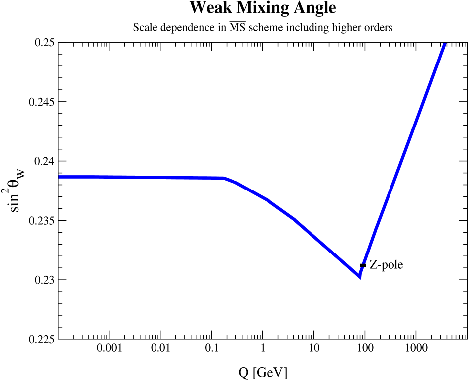
Figure 1: Scale dependence of the weak mixing angle in the $\overline{\rm MS}$ renormalization scheme.

As a particular application, we obtained a definition of the mixing angle in the Thomson limit, $\sin^{2}\theta_{W}\equiv\sin^{2}\hat{\theta}_{W}(0)$ whose relation with the value determined at the $Z$-pole $\sin^{2}\hat{\theta}_{W}(M_{Z})$ is the electroweak analog of the relation between the fine structure $\alpha=\hat{\alpha}(0)$ constant and $\hat{\alpha}(M_{Z})$. This definition also coincides with the gauge invariant definition recently constructed in Ref. [36], and its numerical value is

$$\sin^{2}\theta_{W}=0.23867\pm 0.00016,$$ (64)

where the error is dominated by the experimental error from $Z$ pole measurements. From its relation to the $\overline{\rm MS}$-scheme mixing angle at the $Z$ scale, $\sin^{2}\hat{\theta}_{W}(M_{Z})$, by Eq. (7), we obtain

$$\Delta\hat{\kappa}(0)=0.03232\pm 0.00029,$$ (65)

where now the error is purely theoretical. Finally, using the relation [48] between $\sin^{2}\hat{\theta}_{W}(M_{Z})$ and the effective leptonic mixing angle, $\sin^{2}\theta_{f}^{\rm\;eff}$, defined in Eq. (5), we obtain,

$$\sin^{2}\theta_{W}-\sin^{2}\theta_{\ell}^{\rm\;eff}=0.00718\pm 0.00007.$$ (66)

The error in this relation (which is the main result of this work) is an order of magnitude below current and anticipated experimental uncertainties and considerably smaller than the uncertainty quoted in Refs. [15].

To illustrate the impact of this result on particular observables, we consider the weak charge of the proton, $Q_{W}(p)$, that will be determined using parity-violating elastic $ep$ scattering at the Jefferson Lab. Up-dating the recent analysis of Ref. [39], we obtain the Standard Model prediction

$$Q_{W}(p) = 0.0713\pm 0.0006~{}({\rm input})\pm 0.0003~{}(\Delta\hat{\kappa})\pm 0.0005~{}(Z\gamma\ {\rm box})\pm 0.0001~{}(WW\ {\rm box})$$ (67)

$$= 0.0713\pm 0.0008,$$

where the experimental uncertainties in $\sin^{2}\hat{\theta}_{W}(M_{Z})$ and $m_{t}$ (“input”), the theoretical hadronic uncertainties in $\Delta\hat{\kappa}(0)$ and the $Z\gamma$ box graph, and the uncertainty from unknown higher-order perturbative QCD contributions to the $WW$ box graphs are shown separately and combined in quadrature in the second line. Use of the previous estimate for the uncertainty in $\Delta\hat{\kappa}(0)$ of $\pm 0.0025$ would lead to a theoretical (total) error in the $Q_{W}(p)$ prediction roughly five (three) times larger than in Eq. (67), and in this case, one could neglect the uncertainties associated with other radiative corrections. In light of our analysis, however, the uncertainty in the Standard Model prediction is now three and a half times smaller than the anticipated experimental error, and theoretical uncertainties associated with hadronic contributions to other radiative corrections become relatively more important.

In the same vein, the interpretation of the prospective parity violating deep inelastic measurements will require a careful analysis of higher twist and isospin breaking corrections, especially given that the latter may be responsible for the present discrepancy between the NuTeV result for $\sin^{2}\hat{\theta}_{W}(\mu\sim 3\ {\rm GeV})$ and the SM prediction. Our analysis applies to the deep inelastic regime, as well, where due to the higher energies involved, the uncertainty in $\sin^{2}\hat{\theta}_{W}(\mu)$ is even much smaller since no complications from non-perturbative contributions arise in this case. Given the level of experimental effort required to carry out these precise low energy measurements, performing a theoretical analysis of these effects at the level we have attempted to do here for the weak mixing angle seems well-worth the effort.

Appendix A Updated value for the mixing angle $\epsilon$

Here we determine the phenomenological value of the $\omega$-$\phi$ mixing angle, $\epsilon$, defined by,

$$|\omega\rangle=\cos\epsilon{|\bar{u}u\rangle+|\bar{d}d\rangle\over\sqrt{2}}-\sin\epsilon|\bar{s}s\rangle,\hskip 50.0pt|\phi\rangle=\sin\epsilon{|\bar{u}u\rangle+|\bar{d}d\rangle\over\sqrt{2}}+\cos\epsilon|\bar{s}s\rangle,$$ (68)

where $\epsilon=0$ is referred to as ideal mixing. One way to extract it is to use $SU(3)$ flavor symmetry and first order breaking applied to the vector meson octet mass spectrum. An advantage of this method is that it can be calibrated against the ground state baryon octet, for which Fermi statistics precludes the mixing with an $SU(3)$ singlet state. The mass of the $SU(2)$ singlet, $M_{\Lambda}$, is therefore predicted in terms of the masses of the other electrically neutral octet members,

$$M_{\Lambda}={1\over 3}(2M_{n}+2M_{\Xi^{0}}-M_{\Sigma^{0}})=1105.4\mbox{ MeV},$$ (69)

which reproduces the experimental value [40], $M_{\Lambda}=1115.7$ MeV, within 0.93%. Analogously, the Gell-Mann-Okubo mass formula [41, 42] yields the octet-octet component of the mass matrix for the isosinglet ground state vector mesons,

$$\bar{M}_{88}^{2}={1\over 3}(4\bar{M}^{2}_{K^{*0}}-\bar{M}^{2}_{\rho^{0}})=(933.69\mbox{ MeV})^{2}\times[1\pm 0.0008\pm 0.0020\pm 0.0121\pm 0.0093].$$ (70)

The first error is from the experimental uncertainty in the masses, which are taken from Ref. [40] except for the mass, $M_{\rho^{0}}=775.74\pm 0.65$ MeV, and the width, $\Gamma_{\rho^{0}}=145.3\pm 1.4$ MeV, of the $\rho^{0}$ resonance for which we averaged Refs. [43, 44]. The broadness of some of the resonances involved introduces an ambiguity as for what definition of mass one should use in the Gell-Mann-Okubo formula. For the central value we have chosen the peak position,

$$\bar{M}={M\over\sqrt[4]{1+{\Gamma^{2}\over M^{2}}}},$$ (71)

where $M$ and $\Gamma$ correspond to the usual definition of a relativistic Breit-Wigner resonance form with an $s$-dependent width, i.e. the one used by the Particle Data Group [40]. The second error in Eq. (70) reflects the size of the shift obtained by replacing $\bar{M}$ by $M$. The third error is due to possible isospin breaking effects which we estimated by using $\bar{M}^{2}_{K^{*\pm}}$ in place of $\bar{M}^{2}_{K^{*0}}$. The last error quantifies the limitation of the method and is given by the calibration against the baryon octet as discussed above. Adding all errors in quadrature, we obtain for the $SU(3)$ octet-singlet mixing angle [40], $\theta_{V}$,

$$\tan^{2}\theta_{V}=\frac{\bar{M}_{88}^{2}-\bar{M}_{\phi}^{2}}{\bar{M}_{\omega}^{2}-\bar{M}_{88}^{2}}=0.646^{-0.081}_{+0.090},$$ (72)

which translates into the two solutions, $\epsilon_{1}=0.061\mp 0.032$ and $\epsilon_{2}=-1.292\pm 0.032$. Alternatively, one can compare the branching ratios of the $\omega$ and $\phi$ resonances decaying into $\pi^{0}\gamma$ [45],

$$\tan^{2}\epsilon={M_{\phi}^{3}\over M_{\omega}^{3}}\left(\frac{M_{\omega}^{2}-M_{\pi^{0}}^{2}}{M_{\phi}^{2}-M_{\pi^{0}}^{2}}\right)^{3}\frac{{\cal B}(\phi\to\pi^{0}\gamma)}{{\cal B}(\omega\to\pi^{0}\gamma)}{\Gamma_{\phi}\over\Gamma_{\omega}}=(3.01\pm 0.26)\times 10^{-3},$$ (73)

which gives, $|\epsilon|=0.0548\pm 0.0024$. Comparison with the previous method singles out the solution,

$$\epsilon=+0.0548\pm 0.0024.$$ (74)

The sign and magnitude are also consistent with various other methods [46] and the previous analysis in Ref. [45].

Appendix B Phenomenological approach to OZI suppression

In Section 6 we argued that the OZI rule can at least partly be understood as a result of group theoretical suppression factors relative to OZI allowed processes. Using the result of Appendix A, we now wish to study OZI rule violating contributions to the mass matrix of ground state vector mesons. These mesons dominate the electromagnetic current correlator at hadronic scales, and should therefore serve as a means to quantify OZI rule suppressions phenomenologically. Throughout this Appendix we work in the isospin symmetric limit.

In the flavor basis, $(|\bar{u}u\rangle,|\bar{d}d\rangle,|\bar{s}s\rangle)$, we write the mass matrix in a form which is similar to the one discussed in Ref. [47],

$$M=\left(\begin{array}[]{ccc}A+B&B&B+C\\ B&A+B&B+C\\ B+C&B+C&A+B+D\end{array}\right).$$ (75)

The parameters $A$ and $B$ respect $SU(3)$ symmetry, while $C$ and $D$ break it. The off-diagonal elements, $B$ and $C$, parametrize flavor transitions, and can only be generated by QCD annihilation (singlet) diagrams. The parameter $D$ receives contributions from the strange quark mass, as well as dynamical contributions of both singlet and non-singlet type. The difference to Ref. [47] is that there $C=0$, and $B=B(\mu)$ is a scale dependent singlet function, while we define all entries of $M$ as constants without specifying their relation to the scale dependent current correlators. In the isospin basis, $(|(\bar{u}u-\bar{d}d)/\sqrt{2}\rangle,|(\bar{u}u+\bar{d}d)/\sqrt{2}\rangle,|\bar{s}s\rangle)$, $M$ reads,

$$M=\left(\begin{array}[]{ccc}A&0&0\\ 0&A+2B&\sqrt{2}(B+C)\\ 0&\sqrt{2}(B+C)&A+B+D\end{array}\right),$$ (76)

so that we can identify, $A=\bar{M}^{2}_{\rho^{0}}$. The trace of $M$ then yields the condition,

$$3B+D=\bar{M}^{2}_{\omega}+\bar{M}^{2}_{\phi}-2\bar{M}^{2}_{\rho^{0}},$$ (77)

and $\epsilon$ obtained in Appendix A gives the constraint,

$$\tan 2\epsilon=\sqrt{8}{B+C\over D-B}.$$ (78)

The final relation,

$$(\bar{M}^{2}_{\phi}-\bar{M}^{2}_{\omega})^{2}=\left[3(B+C)-{1\over 3}(C+D)\right]^{2}+{8\over 9}(C+D)^{2},$$ (79)

shows that in the $SU(3)$ limit, $C=D=0$, singlet diagrams associated with $B$ would split $M^{2}_{\phi}$ from $M^{2}_{\rho^{0}}=M^{2}_{\omega}$ in much the same way as triangle anomaly diagrams would split $M^{2}_{\eta^{\prime}}$ from $M^{2}_{\eta}=M^{2}_{\pi}$. Taking into account that $\epsilon\ll 1$, we can approximate,

$$B\approx{\bar{M}^{2}_{\omega}-\bar{M}^{2}_{\rho^{0}}\over 2},\hskip 100.0ptD\approx\bar{M}^{2}_{\phi}-{\bar{M}^{2}_{\omega}+\bar{M}^{2}_{\rho^{0}}\over 2},$$ (80)

which is correct up to ${\cal O}(\epsilon^{2})$. Thus, in the limit of ideal mixing, $B$ drives the splitting of $M^{2}_{\omega}$ from $M^{2}_{\rho^{0}}$ instead. In any case, the singlet contribution associated to $B$ is very small compared to $A$ and $D$. More relevant for this work is the $SU(3)$ breaking singlet parameter,

$$C\approx{\bar{M}^{2}_{\phi}-\bar{M}^{2}_{\omega}\over\sqrt{8}}\tan 2\epsilon-{\bar{M}^{2}_{\omega}-\bar{M}^{2}_{\rho^{0}}\over 2},$$ (81)

which reduces to $C=-B$ in the ideal mixing case, $\epsilon=0$. Numerically, we have,

$$\begin{array}[]{ll}A=(769\mbox{ MeV})^{2},&B=(105\mbox{ MeV})^{2},\\ C=(\;\;74\mbox{ MeV})^{2},&D=(660\mbox{ MeV})^{2}.\end{array}$$ (82)

There is a second solution in which $|B|$, $|C|$, and $|D|$ are all comparable and where $B\approx-C$ to ensure $\epsilon\ll 1$. It also has $D<0$, although the strange quark mass is expected to give the dominant (positive) contribution. Therefore we discard this solution. We can also roughly estimate the singlet component contained in $D$ by relating it to $M_{K^{*0}}$,

$$D_{\rm singlet}\sim D-2(\bar{M}^{2}_{K^{*0}}-\bar{M}^{2}_{\rho^{0}})=(123\mbox{ MeV})^{2},$$ (83)

which is of similar size as $B$ and $C$. Thus, singlet contributions to vector meson masses are generally suppressed by more than an order of magnitude beyond the QCD suppression factors discussed in Section 6 indicating that the smallness of the known coefficient, $C_{2}\ll 1$, may indeed be a generic feature that persists at higher orders. Qualitatively the same results are obtained if linear mass relations are used in place of masses squared, except that singlet contributions appear even more suppressed.

References

- [1] M. J. G. Veltman, Nucl. Phys. B 123, 89 (1977).
- [2] W. A. Bardeen, A. J. Buras, D. W. Duke and T. Muta, Phys. Rev. D 18, 3998 (1978).
- [3] S. Weinberg, Phys. Lett. B 91, 51 (1980).
- [4] W. J. Marciano and A. Sirlin, Phys. Rev. Lett. 46, 163 (1981).
- [5] W. J. Marciano and J. L. Rosner, Phys. Rev. Lett. 65, 2963 (1990) and Erratum ibid. 68, 898 (1992).
- [6] S. Fanchiotti, B. A. Kniehl and A. Sirlin, Phys. Rev. D 48, 307 (1993).
- [7] C. S. Wood et al., Science 275, 1759 (1997).
- [8] SLAC–E–158 Collaboration: P. L. Anthony et al., Phys. Rev. Lett. 92, 181602 (2004) and hep-ex/0504049.
- [9] Qweak Collaboration: D. S. Armstrong et al., AIP Conf. Proc. 698, 172 (2004).
- [10] A. Czarnecki and W. J. Marciano, Phys. Rev. D 53, 1066 (1996).
- [11] A. Czarnecki and W. J. Marciano, Int. J. Mod. Phys. A 15, 2365 (2000).
- [12] M. J. Musolf and B. R. Holstein, Phys. Lett. B 242, 461 (1990).
- [13] M. J. Musolf and B. R. Holstein, Phys. Rev. D 43, 2956 (1991).
- [14] W. J. Marciano and A. Sirlin, Phys. Rev. D 22, 2695 (1980) and Erratum ibid. 31, 213 (1985).
- [15] W. J. Marciano, Radiative Corrections to Neutral Current Processes, p. 170 in Ref. [35].
- [16] NuTeV Collaboration: G. P. Zeller et al., Phys. Rev. Lett. 88, 091802 (2002) and Erratum ibid. 90, 239902 (2003).
- [17] S. G. Gorishnii, A. L. Kataev and S. A. Larin, Phys. Lett. B 212, 238 (1988) and ibid. 259, 144 (1991).
- [18] L. R. Surguladze and M. A. Samuel, Phys. Rev. Lett. 66, 560 (1991) and Erratum ibid. 66, 2416 (1991).
- [19] S. A. Larin, T. van Ritbergen and J. A. M. Vermaseren, Nucl. Phys. B 438, 278 (1995).
- [20] K. G. Chetyrkin, J. H. Kühn and M. Steinhauser, Nucl. Phys. B 482, 213 (1996).
- [21] J. Erler, Phys. Rev. D 59, 054008 (1999).
- [22] L. J. Hall, Nucl. Phys. B 178, 75 (1981).
- [23] I. Antoniadis, C. Kounnas and K. Tamvakis, Phys. Lett. B 119, 377 (1982).
- [24] P. Langacker and N. Polonsky, Phys. Rev. D 47, 4028 (1993).
- [25] F. Jegerlehner, Renormalizing the Standard Model, p. 476 in Ref. [26].
- [26] M. Cveti and P. Langacker, Testing the Standard Model, Proceedings of the Theoretical Advanced Study Institute in Elementary Particle Physics, Boulder, USA, June 3–27 (1990).
- [27] M. Davier and A. Höcker, Phys. Lett. B 435, 427 (1998).
- [28] M. Davier, S. Eidelman, A. Höcker and Z. Zhang, Eur. Phys. J. C 31, 503 (2003).
- [29] B. A. Kniehl, Phys. Lett. B 237, 127 (1990).
- [30] A. H. Hoang, M. Jezabek, J. H. Kühn and T. Teubner, Phys. Lett. B 338, 330 (1994).
- [31] S. Okubo, Phys. Lett. 5, 165 (1963).
- [32] G. Zweig, An SU(3) Model For Strong Interaction Symmetry And Its Breaking, 2, CERN Report No. 8419/TH 412 (1964).
- [33] J. Iizuka, Prog. Theor. Phys. Suppl. 37, 21 (1966).
- [34] T. van Ritbergen, A. N. Schellekens and J. A. M. Vermaseren, Int. J. Mod. Phys. A 14, 41 (1999).
- [35] P. Langacker, Precision Tests of the Standard Electroweak Model, Advanced series on directions in high energy physics: 14 (World Scientific, Singapore, Singapore, 1995).
- [36] A. Ferroglia, G. Ossola and A. Sirlin, Eur. Phys. J. C 34, 165 (2004).
- [37] G. Degrassi and A. Sirlin, Phys. Rev. D 46, 3104 (1992).
- [38] D. R. T. Jones, Phys. Rev. D 25, 581 (1982).
- [39] J. Erler, A. Kurylov and M. J. Ramsey-Musolf, Phys. Rev. D 68, 016006 (2003).
- [40] Particle Data Group: S. Eidelman et al., Phys. Lett. B 592, 1 (2004).
- [41] S. Okubo, Prog. Theor. Phys. 27, 949 (1962).
- [42] M. Gell-Mann, Phys. Rev. 125, 1067 (1962).
- [43] L. M. Barkov et al., Nucl. Phys. B 256, 365 (1985).
- [44] CMD-2 Collaboration: R. R. Akhmetshin et al., Phys. Lett. B 578, 285 (2004).
- [45] P. Jain et al., Phys. Rev. D 37, 3252 (1988).
- [46] J. Arafune, M. Fukugita and Y. Oyanagi, Phys. Lett. B 70, 221 (1977).
- [47] A. De Rujula, H. Georgi and S. L. Glashow, Phys. Rev. D 12, 147 (1975).
- [48] P. Gambino and A. Sirlin, Phys. Rev. D 49, 1160 (1994).