Multiplicities and bulk thermodynamic quantities at $\sqrt{s_{NN}}=130$ GeV with SHARE

Abstract

We introduce the Statistical Hadronization with Resonances (SHARE) suite of programs and perform a study of particle multiplicities as well as bulk thermodynamic quantities for the RHIC Au–Au reactions at $\sqrt{s_{NN}}=130$ GeV. We also show that the statistical hadronization model, with parameters fitted to match pion, proton and hyperon ratios, in turn correctly and consistently reproduces rapidity particle multiplicity.

,

.

1 Introduction

The statistical hadronization model [1, 2] has been used extensively to study soft strongly interacting particle production since the 1950s. When the full spectrum of strongly interacting resonances is included [3], this approach is capable to describe the abundances and spectra of the produced particles in detail. The emitted particles carry information about the gross features of the hadron source. Their study allows precise extrapolation to unmeasured particles and/or kinematic domains, allowing understanding of bulk properties of hadronizing matter such as particle multiplicity, mean energy per particle, specific per baryon entropy etc. Once hadron spectra are understood, information about the dynamical properties such as collective flow of hadronizing matter becomes accessible.

Other important physical information is contained in the statistical model parameters obtained fitting measured particle ratios. These offer additional insights, for example one may want to relate the chemical (particle production) freeze-out temperature to the phase transformation temperature of the deconfined quark–gluon plasma (QGP) phase into hadrons. The chemical freeze-out temperature also helps understand the percentage of total particles which originated from resonance decays. The chemical freeze-out parameters fix e.g. the charged and neutral hadronic multiplicities, flavor density, baryon stopping, and so on.

To properly address these issues, standardization of the technical and mathematical tools employed in statistical hadronization studies has to occur. Furthermore the model differences have to be understood and the different versions have to be unified. Here, we note the chemical equilibrium version, where all (light and strange) flavor yields are assumed to have evolved for a long time in the hadron phase reaching equilibrium yield [4, 5, 6]. More refined approaches allow for an under-saturation of the strangeness quantum number [7], implemented quantitatively by a parameter $\gamma_{s}$ (assumed to be $<1$) which affects both $s$ and $\overline{s}$ in the same way ($\gamma_{s}=\gamma_{\overline{s}}$, in contrast to the fugacity $\lambda_{s}=\lambda_{\overline{s}}^{-1}$). The simplest physical scenario applicable here is that the hadron source does not live for long enough for strangeness production to approach chemical equilibration (Fig. 1 left), while the more rapidly evolving light flavor yields had time to equilibrate.

The third model approach is to allow for chemical non-equilibrium also in the light flavor yield. This situation is most likely to be found in a reaction scenario involving formation of the QGP. Namely, the phase space density of flavors in QGP is higher than of a equilibrated hadron gas in the physical domain explored today at SPS and at RHIC [8]. This is illustrated in Fig. 1 in the right panel, where we show that the phase space density difference compensation leads to a step-up in the quark flavor occupancy parameter $\gamma$.

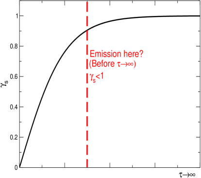
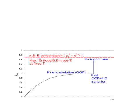
Figure 1: Chemical non-equilibrium can arise out of kinetic evolution (left), and in rapid QGP freeze-out into hadrons (right).

Linked to the question of chemical equilibration is the timescale between hadronization (the moment at which degrees of freedom become hadronic) and freeze-out (the moment at which hadrons stop interacting). It is generally assumed that there are two freeze-outs, chemical and thermal, the former corresponding to particle production and latter to spectral shape generated by elastic hadron–hadron scattering. Chemical equilibration requires slow evolution of the hadronic gas system, hence to a situation in which hadronization and freeze-out are well separated, and considerable modification of all hadronic yields could occur in the interacting hadron gas phase [4]. In such a scenario one also expects that the thermal freeze-out is clearly different from the chemical freeze-out.

If QGP hadronizes, the difference between quark and hadron phase spaces makes it likely that a sudden freeze-out will occur creating initially hadrons in chemical non-equilibrium; In particular, the high entropy density of a QGP phase with massless degrees of freedom accompanied by the rapid matter flow driven by the high internal pressure makes it reasonable that hadrons are produced in a fast phase transformation, which leads to flavor over-saturated state [8], with more $q\overline{q}$ and $s\overline{s}$ pairs than is expected at chemical equilibrium. It is necessary to ascertain phenomenologically whether, in fact, one needs non-equilibrium to account for particle abundances in heavy ion collisions. The Statistical Hadronization with Resonances (SHARE) package has been developed allowing to resolve this ambiguity as one of the tasks

In the following section we give introduce the statistical model, and the details implemented in SHARE. We refer the user to Ref. [9] for a detailed presentation and user’s manual. This is followed in section 3 by discussion of our results, addressing in turn particle ratios and bulk properties.

2 Main SHARE features

Many of our experimental friends present at this meeting can obtain on back of an envelope the statistical yield of stable hadrons. SHARE extends this to include important refinements capable to change these results significantly.

2.1 Particle yields allow quantum statistics and chemical non-equilibrium

The Grand-Canonical statistical prescription assumes that enough particles of each flavor are produced to keep fluctuations of each quantum number small, and the system volume reduces to a “large” normalization constant. This requirement, together with entropy maximization, leads to the Fermi–Dirac or Bose–Einstein distribution functions for densities of particle species $i$:

$$n(m_{i},g_{i};T,\Upsilon_{i})\equiv n_{i} = g_{i}\int{d^{3}p\over(2\pi)^{3}}{1\over\Upsilon^{-1}_{i}\exp(\sqrt{p^{2}+m^{2}_{i}}/T)\pm 1},$$ (1)

$$= \frac{g_{i}}{2\pi^{2}}\sum_{n=1}^{\infty}(\mp)^{n-1}\Upsilon_{i}^{n}\,\frac{T\,m_{i}^{2}}{n}\,K_{2}\left(\frac{nm_{i}}{T}\right).$$ (2)

In Eq. (2), the upper signs refer to fermions and the lower signs to bosons, respectively. $\Upsilon_{i}$ is the fugacity factor, and $m_{i}$ is the particle mass. The quantity $g_{i}=(2J_{i}+1)$ is the spin degeneracy factor as we distinguish all particles according to their electrical charge and mass. The index $i$ labels different particle species, including hadrons which are stable under strong interactions (such as pions, kaons, nucleons or hyperons) and hadron which are unstable ($\rho$ mesons, $\Delta(1232)$, etc.). The second form, Eq. (2), expresses the momentum integrals in terms of the modified Bessel function $K_{2}$. This form is practical in the numerical calculations and is used in the SHARE code. Although in principle in some limiting cases this is not a convergent expansion, this is a rare exception: the series expansion (sum over $n$) converges when $\Upsilon_{i}e^{-m_{i}/T}<1$. Violation of this condition occurs in practical context only for the pion case within the range of parameters of interest.

In the most general chemical condition, the fugacity is defined through the parameters $\lambda_{I^{\,i}_{3}},\lambda_{q},\lambda_{s},\lambda_{c}$ (expressing, respectively, the isospin, light, strange and charm quark fugacity factors), and $\gamma_{q},\gamma_{s},\gamma_{c}$ (expressing the light, strange and charm quark phase space occupancies, $=1$ for absolute yield equilibrium). The fugacity $\Upsilon_{i}$ is then given by:

$$\Upsilon_{i}=\lambda_{I^{i}_{3}}\left(\lambda_{q}\gamma_{q}\right)^{N^{i}_{q}}\left(\lambda_{s}\gamma_{s}\right)^{N^{i}_{s}}\left(\lambda_{c}\gamma_{c}\right)^{N^{i}_{c}}\left(\lambda_{\bar{q}}\gamma_{\bar{q}}\right)^{N^{i}_{\bar{q}}}\left(\lambda_{\bar{s}}\gamma_{\bar{s}}\right)^{N^{i}_{\bar{s}}}\left(\lambda_{\bar{c}}\gamma_{\bar{c}}\right)^{N^{i}_{\bar{c}}},$$ (3)

where

$$\lambda_{q}=\lambda^{-1}_{\bar{q}},\qquad\lambda_{s}=\lambda^{-1}_{\bar{s}},\qquad\lambda_{c}=\lambda^{-1}_{\bar{c}},\qquad$$ (4)

and

$$\gamma_{q}=\gamma_{\bar{q}},\qquad\gamma_{s}=\gamma_{\bar{s}},\qquad\gamma_{c}=\gamma_{\bar{c}}.$$ (5)

Here, $N^{i}_{q}$, $N^{i}_{s}$ and $N^{i}_{c}$ are the numbers of light $(u,d)$, strange $(s)$ and charm $(c)$ quarks in the $i$th hadron, and $N^{i}_{\bar{q}}$, $N^{i}_{\bar{s}}$ and $N^{i}_{\bar{c}}$ are the numbers of the corresponding antiquarks in the same hadron.

2.2 Particle yields from resonance decays

At first, we consider hadronic resonances as if they were particles with a given well defined mass, e.g., their decay width is insignificant. All hadronic resonances decay rapidly after freeze-out, feeding the stable particle abundances. Moreover, heavy resonances may decay in cascades, which are implemented in the algorithm where all decays proceed sequentially from the heaviest to lightest particles. As a consequence, the light particles obtain contributions from the heavier particles, which have the form

$$n_{1} = b_{2\rightarrow 1}\,...\,b_{N\rightarrow N-1}n_{N},$$ (6)

where $b_{k\rightarrow k-1}$ combines the branching ratio for the $k\rightarrow k-1$ decay (appearing in [10]) with the appropriate Clebsch–Gordan coefficient. The latter accounts for the isospin symmetry in strong decays and allows us to treat separately different charged states of isospin multiplets of particles such as nucleons, Deltas, pions, kaons, etc. For example, different isospin multiplet member states of $\Delta$ decay according to the following pattern:

$$\Delta^{++}\rightarrow\pi^{+}+p,$$ (7)

$$\Delta^{+}\rightarrow{1\over 3}(\pi^{+}+n)+{2\over 3}(\pi^{0}+p),$$ (8)

$$\Delta^{0}\rightarrow{1\over 3}(\pi^{-}+p)+{2\over 3}(\pi^{0}+n),$$ (9)

$$\Delta^{-}\rightarrow\pi^{-}+n.$$ (10)

Here, the branching ratio is 1 but the Clebsch–Gordan coefficients introduce another factor leading to the effective branching ratios of 1/3 or 2/3, where appropriate.

To implement this procedure on every particle, one needs to keep in mind that the partial widths (product of branching ratio with total width) are often not sufficiently well known. In addition, in case of weak decays, an experiment-specific acceptance coefficient is needed to correctly model the observed particle rate. This introduces implementation dependent variances of statistical hadronization. To combat invisible model variations we suggest an open-source “standard”, where resonance decay trees are kept on record and can be updated in a transparent fashion, and weak acceptances can be set to correspond to needs of each experiment. This is the SHARE code [9].

In SHARE, as a rule, all decays with the branching ratios smaller than 1% are disregarded. In addition, if the decay channels are classified as dominant, large, seen, or possibly seen, the most important channel is taken into account. If two or more channels are said to be equally important, we take all of them with the same weight. For example $f_{0}(980)$ decays into $\pi\pi$ (according to [10] this is the dominant channel) and $K\overline{K}$ (according to [10] this is the seen channel). In our approach, according to the rules stated above, we include only the process $f_{0}(980)\longrightarrow\pi\pi$. Similarly, $a_{0}(1450)$ has three decay channels: $\eta\pi$ (seen), $\pi\eta^{\prime}(958)$ (seen), and $K\overline{K}$ (again seen). In this case, we include all three decay channels with the weight (branching ratio) 1/3. A table of allowed decays and branching ratios is provided and can be updated. Users can modify this table to study the magnitude of systematic error introduced by incomplete knowledge of both resonance masses and decay parameters.

2.3 Hadron yields allowing for finite resonance width

If the particle $i$ has a finite width $\Gamma_{i}$, the thermal yield of the particle is more appropriately obtained by weighting Eq. (1) over a range of masses to take the mass spread into account:

$$\tilde{n}_{i}^{\Gamma}=\int\!dM\,n(M,g_{i};T,\Upsilon_{i})\frac{1}{2\pi}\frac{\Gamma_{i}}{(M-m_{i})^{2}+\Gamma_{i}^{2}/4}\to n_{i},\mbox{\ \ for\ \ }\Gamma_{i}\to 0.$$ (11)

The use of the Breit–Wigner distribution with energy independent width means that there is a finite probability that the resonance would be formed at unrealistically small masses. Since the weight involves a thermal distribution $n(M,g_{i};T,\Upsilon_{i})$ which would contribute in this unphysical domain, one must use, in Eq. (11), an energy dependent width.

The dominant energy dependence of the width is due to the decay threshold energy phase space factor, dependent on the angular momentum present in the decay. The explicit form can be seen in the corresponding reverse production cross sections [11, 12]. The energy dependent partial width in the channel $i\to j$ is to a good approximation:

$$\Gamma_{i\to j}(M)=b_{i\to j}\Gamma_{i}\left[1-\left(\frac{m_{ij}}{M}\right)^{2}\right]^{l_{ij}+\frac{1}{2}},\quad\mbox{for}\quad M>m_{ij}.$$ (12)

Here, $m_{ij}$ is the threshold of the decay reaction with branching ratio $b_{i\to j}$. For example for the decay of $i:=\Delta^{++}$ into $j:=p+\pi^{+}$, we have $m_{ij}=m_{p}+m_{\pi^{+}}$, while the branching ratio is unity and the angular momentum released in decay is $l_{ij}=1$. From these partial widths the total energy dependent width arises,

$$\Gamma_{i}\to\Gamma_{i}(M)=\sum_{j}\Gamma_{i\to j}(M).$$ (13)

For a resonance with width, we thus have replacing Eq. (11):

$$n_{i}^{\Gamma}=\frac{1}{N_{i}}\sum_{j}\int_{m_{ij}}^{\infty}dM\,n(M,g_{i};T,\Upsilon_{i})\frac{\Gamma_{i\to j}(M)}{(M-m_{i})^{2}+[\Gamma_{i}(M)]^{2}/4},$$ (14)

and the factor $N$ (replacing $2\pi$) ensures the normalization:

$$N_{i}=\sum_{j}\int_{m_{ij}}^{\infty}dM\frac{\Gamma_{i\to j}(M)}{(M-m_{i})^{2}+[\Gamma_{i}(M)]^{2}/4}.$$ (15)

In principle, Eq. (14) does not take into account the possibility that the state into which one is decaying is itself a unstable state in a thermal bath. Doing this would require a further average over the width distribution of receiving state. This higher order effect is at present not implemented in SHARE.

2.4 Canonical effects

We did not address in SHARE refinement specific to small particle numbers where the grand canonical phase space description fails [14]. Thus SHARE is geared to describe particle multiplicities where within the causal interaction domain there is an effective ‘particle’ heat bath. To be more specific, the grand canonical phase space will yield correctly e.g. the $\overline{\Omega}$ yield in the limit that the number of strange quark pairs significantly exceeds those required to make this particle, e.g. we need about 10 $s\bar{s}$ pairs. Without doubt these are the conditions prevailing in the physical environment we are exploring here, since at RHIC 130GeV about 8 strange quark pairs are produced per each participating baryon [15, 16], and baryon density is about 25 per unit of rapidity.

3 RHIC 130 fit results

3.1 Particle ratios

We study particle ratios taken at different though similar collision centralities, e,g, 5%, 6%, 8%, 10%. In first and hopefully good approximation we expect that the physical conditions established are similar in all these case. In other words we expect that for particle yields in the statistical model to be consistent:

• The volume should appear as a normalization constant. Temperature and the other thermal parameters should be, within error, independent of the centrality for a range of centralities.

• This normalization constant should present an approximately proportional dependence on the total charge multiplicity.

These requirements can be tested by fitting the total particle multiplicity of a range of experimentally measured centrality bins, together with a set of hadron ratios (Fig 3). We consider seven most central bins, as measured by STAR, [17], and find no significant variation of the fitted bulk parameters ($T,\lambda_{q,s},\gamma_{q,s},\lambda_{I3}$) and their errors. The only parameter in the fit which does vary from bin to bin is the absolute normalization, needed to describe the charged multiplicities; It’s statistical significance profiles are shown in Fig. 2 (left); As noted elsewhere [8, 13], introducing $\gamma_{q}$ significantly and consistently improves the statistical significance of the fit.

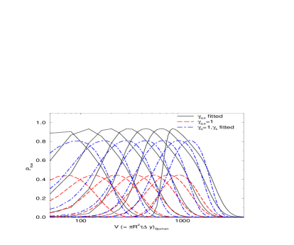
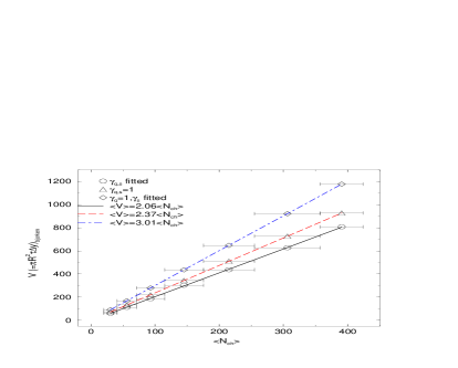
Figure 2: Statistical significance profiles for volume for different centralities (left), and it’s correlation with the charged particle number (right).

When the fitted volume normalization parameter is plotted against the mean charged particle multiplicity, an approximately linear dependence is observed for all models (Fig. 2 right). Light quark non-equilibrium decreases the necessary volume by as much as 30 $\%$. While this is predictable, since the non-equilibrium model invariably leads to quark over-saturation ($\gamma_{q}>1$) at high energies and thus higher particle density [8]. The smaller volume required in non-equilibrium has not as yet been subject to an in-depth analysis, particularly in light of the HBT puzzle [18]: It is sometimes thought that an explosive hadronization scenario is ruled out by HBT measurements [19]. However, as this study the non-equilibrium particle production is yielding a higher density than that predicted by equilibrium hydrodynamics models, which should rectify this discrepancy.

We have used RHIC ratios (130 GeV) to calculate thermal parameters within each model. While a plot, showing a model-data comparison, is given in Fig. 3 and table 1, we refer the reader to [13] for an in-depth data and statistical significance analysis of the fits.

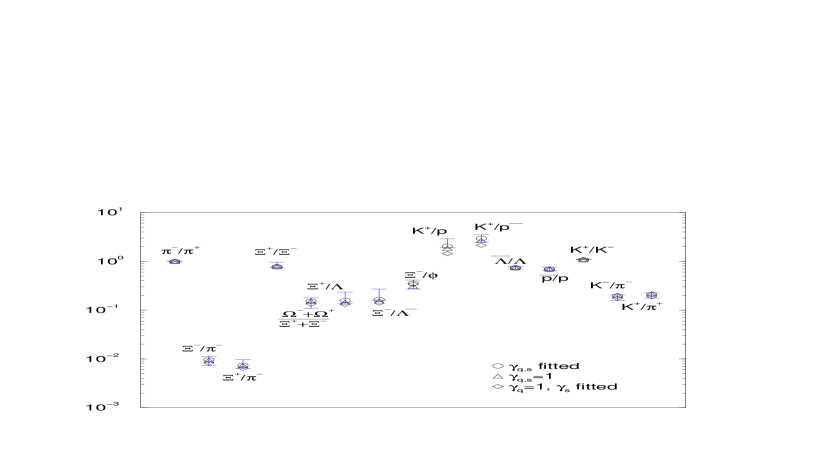
Figure 3: The best fits to hadron yields at RHIC-130 GeV. See table 1 for parameters of the fits and statistical significance.

Table 1: RHIC-130 GeV hadronization parameters

	$\gamma_{q,s}$ vary		$\gamma_{q,s}=1$		$\gamma_{q}=1$, $\gamma_{s}$ varies
parameter	$\Gamma=0$	$\Gamma$ [10]	$\Gamma=0$	$\Gamma$ [10]	$\Gamma=0$	$\Gamma$ [10]
T [MeV]	133 $\pm$ 10	135 $\pm$ 12	158 $\pm$ 13	0.157 $\pm$ 15	152 $\pm$ 16	153 $\pm$ 23
$10^{4}(\lambda_{q}-1)$	708 $\pm$ 342	703 $\pm$ 337	735 $\pm$ 390	730 $\pm$ 382	724 $\pm$ 373	721 $\pm$ 363
$\lambda_{s}$	1.03132973	1.03203555	1.02636207	1.02788897	1.0295346	1.0300848
$\gamma_{q}$	1.66 $\pm$ 0.013	1.65 $\pm$ 0.030	1	1	1	1
$\gamma_{s}$	2.41 $\pm$ 0.61	2.28 $\pm$ 0.46	1	1	1.17 $\pm$ 0.30	1.10 $\pm$ 0.25
$10^{4}(\lambda_{I_{3}}-1)$	30 $\pm$ 305	28 $\pm$ 293	59 $\pm$ 564	53 $\pm$ 508	64 $\pm$ 525	59 $\pm$ 481
	fit relevance
$N-p=\mbox{DoF}$	16-5	16-5	16-3	16-3	16-4	16-4
$\chi^{2}/$DoF	0.4243	0.4554	1.0255	0.8832	0.6067	0.7301
significance	0.9461	0.9307	0.4225	0.5705	0.8385	0.7232

3.2 Bulk quantities

We proceed to calculate $\sqrt{s_{NN}}=130$ GeV Au–Au bulk quantities. The results are shown in table 2. It is immediately apparent that many of the observed quantities depend strongly on whether light quarks are in equilibrium. By contrast, introducing incomplete strange chemical equilibration while maintaining $\gamma_{q}=1$ does not produce a significant shift in the calculated quantities from the full equilibrium values. This is due to the fact that in this case the fit leads to practically fully equilibrated system as within error $\gamma_{s}=1$ results.

Overall, the greatest change is that the entropy density is considerably higher within the $\gamma_{q}\neq 1$ model. This is consistent with the model’s physical motivation, since the high $\gamma_{q}$ is invoked to conserve entropy in a QGP$\rightarrow$ HG transition, without need for a mixed phase and expansion.

Strangeness per entropy, being primarily sensitive to input ratios such as $K/\pi$ (fitted), is not significantly affected by model choice [16, 20]. Quantities such as particle multiplicity per baryon (which follows entropy per baryon), net charge per baryon, and strangeness per baryon, however, vary considerably between models, making them promising probes for statistical model variants involving chemical (non)equilibration. We have also show (last line in table 2 ) that the fraction of particles coming from weak decays varies considerably from model to model, decreasing as non-equilibrium is introduced. This is to be expected, since all non-equilibrium fits yield over-saturated phase space occupancies. These enhance all particles, including resonances, thereby increasing the percentage of particles emitted in strong decays. This feature should also provide a test for non-equilibrium: Since all weak decays, including those which can not be reconstructed, tend to occur at a measurably large distance from the primary vertex, a precise estimate of the number of particles which do not come from the primary vertex could also serve as a potential probe for equilibrated emission.

Due to the higher particle multiplicity in the non-equilibrium case, the thermalized energy per particle goes down. While this model does not include collective (transverse and longitudinal) flow, and hence can not address the total energy in the system (some of which is contained in the collective motion, rather than the internal energy), the discrepancy in the energy per particle can become a strong constraint if the models under consideration are coupled to a model (such as the commonly used “Blast Wave”) incorporating flow. Successful fits of abundances and spectra within the same model have been made both in the equilibrium and non equilibrium cases [21, 5, 22], and it will be interesting to rigorously test those for full energy conservation.

Table 2: RHIC 130 GeV Au–Au best fit bulk quantities ratios, including charged particles ($h^{\pm 0}$,energy ($E$), Baryon/antibaryon ($B,\overline{B}$), strangeness ($s,\overline{s}$) and entropy (S). The bottom ratio refers to the fraction of totally emitted particles which arise out of weak decays (assuming negligible $K_{L}\rightarrow 3\pi$ detectability)

	$\gamma_{q,s}$ vary		$\gamma_{q,s}=1$		$\gamma_{q}=1$, $\gamma_{s}$ varies
ratio	$\Gamma=0$	$\Gamma$ [10]	$\Gamma=0$	$\Gamma$ [10]	$\Gamma=0$	$\Gamma$ [10]
$(h^{+}+h^{-})/(B-\overline{B})$	30.0827	30.821	18.613	20.087	22.149	22.758
$(h^{+}-h^{-})/(B-\overline{B})$	0.618	0.618	0.603	0.602	0.632	0.624
$E/(B-\overline{B})$	37.220	38.152	31.756	33.403	36.004	36.441
$(s+\overline{s})/(B-\overline{B})$	9.771	9.419	6.328	6.517	8.3504	7.862
$S/(B-\overline{B})$	362.679	369.857	236.14	252.001	280.8769	284.407
$(h^{+}+h^{-}+h^{0})/(B-\overline{B})$	71.265	70.996	53.551	54.479	62.108	60.678
$(h^{+}+h^{-}+h^{0})/(h^{+}+h^{-})$	1.6427	1.64	1.6338	1.638	1.6414	1.641
$(h^{+}-h^{-})/(h^{+}+h^{-})$	0.0142	0.0143	0.0184	0.0181	0.0167	0.0169
$E/(h^{+}+h^{-})$	0.858	0.882	0.9689	1.004	0.952	0.986
$(s+\overline{s})/(h^{+}+h^{-})$	0.225	0.218	0.193	0.196	0.221	0.213
$S/(h^{+}+h^{-})$	8.360	8.546	7.205	7.576	7.423	7.696
$E/h^{-}$	1.748	1.796	1.982	2.054	1.943	2.01
$(B-\overline{B})/h^{-}$	0.0469	0.0471	0.0624	0.0612	0.0534	0.0552
$(s+\overline{s})/h^{-}$	0.4588	0.443	0.395	0.401	0.451	0.435
$S/h^{-}$	17.0297	17.417	14.738	15.493	15.161	15.719
$(h^{+}+h^{-}+h^{0})/h^{-}$	3.346	3.341	3.342	3.349	3.352	3.354
$(B+\overline{B})/h^{-}$	0.256	0.256	0.327	0.323	0.289	0.295
$S/(s+\overline{s})$	37.118	39.266	37.314	38.669	33.636	36.176
$S/E$	9.7443	9.694	7.436	7.544	7.801	7.804
$\frac{(h^{+}+h^{-}+h^{0})_{weak}}{(h^{+}+h^{-}+h^{0})_{total}}$	0.325	0.326	0.425	0.427	0.410	0.404

In conclusion, using the SHARE package we have analyzed the Au–Au $\sqrt{s_{NN}}=130$ GeV experimental output with a variety of statistical models. All are able to fit particle ratios and total charged multiplicity, achieving the highest statistical significance with the full non-equilibrium ansatz. We have calculated bulk thermodynamic properties of the system from the fitted parameters, and found that many of these are model dependent, with particularly strong discrepancies between full non-equilibrium ($\gamma_{q,s}\neq 1$) and the rest. We hope that higher statistics and 200 GeV data [13] will be able to falsify some of these models unambiguously, and hence allow a precise determination of the statistical properties of the system.

Acknowledgments

Work supported in part by grants from: the U.S. Department of Energy DE-FG03-95ER40937 and DE-FG02-04ER41318, NATO Science Program PST.CLG.979634, the Natural Sciences and Engineering Research Council of Canada, the Fonds Nature et Technologies of Quebec.
G. Torrieri wishes to thank the organizers of the “Focus on Multiplicity” conference (Bari, 2004), and the Tomlinson Foundation of McGill University for their generous support.

References

References

- [1] E. Fermi, Prog. Theor. Phys. 5, 570 (1950).
- [2] I. Pomeranchuk, Proc. USSR Academy of Sciences (in Russian) 43, 889 (1951).
- [3] R. Hagedorn, Suppl. Nuovo Cimento 2, 147 (1965).
- [4] O. Barannikova [STAR Collaboration], arXiv:nucl-ex/0403014.
- [5] W. Broniowski and W. Florkowski, Phys. Lett. B490, 223 (2000).
- [6] P. Braun-Munzinger, K. Redlich and J. Stachel, arXiv:nucl-th/0304013.
-
[7]
J. Rafelski,
Phys. Lett. B 262, 333 (1991);
J. Letessier, A. Tounsi, U. W. Heinz, J. Sollfrank and J. Rafelski, Phys. Rev. D 51, 3408 (1995) [arXiv:hep-ph/9212210];
F. Becattini, M. Gazdzicki and J. Sollfrank, Eur. Phys. J. C 5, 143 (1998) [arXiv:hep-ph/9710529];
J. Cleymans, B. Kaempfer, P. Steinberg and S. Wheaton, J. Phys. G 30, S595 (2004) [arXiv:hep-ph/0311020]. -
[8]
J. Letessier and J. Rafelski,
Phys. Rev. C 59, 947 (1999)
[arXiv:hep-ph/9806386];
J. Letessier and J. Rafelski, J. Phys. G 25, 295 (1999) [arXiv:hep-ph/9810332];
J. Rafelski and J. Letessier, arXiv:nucl-th/9903018;
J. Rafelski, J. Phys. G 28, 1833 (2002) [arXiv:hep-ph/0112185]. - [9] G. Torrieri, S. Steinke, W. Broniowski, W. Florkowski, J. Letessier and J. Rafelski, arXiv:nucl-th/0404083.
- [10] K. Hagiwara et al., Particle Data Group Collaboration, Phys. Rev. D 66, 010001 (2002), see also earlier versions, note that the MC identification scheme for most hadrons was last presented in 1996.
- [11] H. Terazawa, Phys. Rev. D 51, 954 (1995).
- [12] G. J. Gounaris and J. J. Sakurai, Phys. Rev. Lett. 21, 244 (1968).
- [13] G. Torrieri, J. Rafelski, J. Letessier Statistical Hadronization description of the yields of stable particles and short-lived resonances in 130 and 200 GeV Au-Au collisions, to be published shortly.
-
[14]
J. Rafelski and M. Danos,
Phys. Lett. B 97, 279 (1980);
J. Cleymans, K. Redlich and E. Suhonen, Z. Phys. C 51, 137 (1991);
M. I. Gorenstein, M. Gazdzicki and W. Greiner, Phys. Lett. B 483, 60 (2000) [arXiv:hep-ph/0001112]. - [15] J. Rafelski, J. Letessier and G. Torrieri, Phys. Rev. C 64, 054907 (2001) [Erratum-ibid. C 65, 069902 (2002)] [arXiv:nucl-th/0104042].
- [16] J. Rafelski and J. Letessier, arXiv:hep-ph/0308154 (to appear in proceedings of HADRON2004, Rio de Janeiro).
- [17] J. Adams, [STAR Collaboration], arXiv:nucl-ex/0311017 (submitrted to Phys. Rev. C).
- [18] D. Magestro, arXiv:nucl-ex/0408014.
- [19] L. P. Csernai, M. I. Gorenstein, L. L. Jenkovszky, I. Lovas and V. K. Magas, Phys. Lett. B 551, 121 (2003) [arXiv:hep-ph/0210297].
-
[20]
M. Gazdzicki,
Acta Phys. Polon. B 35 (2004) 187;
J. Rafelski and J. Letessier, Acta Phys. Polon. B 34, 5791 (2003) [arXiv:hep-ph/0309030]. - [21] G. Torrieri and J. Rafelski, New Jour. Phys. 3, 12 (2001) [arXiv:hep-ph/0012102].
- [22] G. Torrieri and J. Rafelski, J. Phys. G 30, S557 (2004) [arXiv:nucl-th/0305071].