Non-Gibbs Particle Spectra from Thermal Equilibrium

Abstract

We propose that transverse momentum spectra with power-law tails observed in ultrarelativistic heavy ion collisions can be interpreted as originating in a medium in thermal equilibrium. General conditions on the dynamical equations are formulated, leading in equilibrium to various energy distributions of particles. Starting with the linear Fokker-Planck equation we analyze conditions for Boltzmann-Gibbs, Tsallis, or other equilibrium distributions based upon the dependence of fluctuation and dissipation on the energy of the observed subsystem. RHIC neutral pion data definitely exclude Boltzmann-Gibbs distribution over the entire range of observed transverse momenta.

I Introduction

There is an increasing interest in phenomena, where a non-conventional equilibrium distribution, different from the Boltzmann-Gibbs (BG) formula Gibbs (1902); Balescu (1975), arises. Like the BG weight, $\exp(-E/T)$, can be derived as the canonical probability starting from Boltzmann’s entropy formula, generalized entropies may lead to other canonical distributions. Frequently discussed suggestions are the Rényi Rényi (1970); Wehrl (1978), or the Daróczy-Tsallis entropy Daroczy (1970); Aczel and Daroczy (1975); Tsallis (1999); Prato and Tsallis (1999); Latora et al. (2001, 2002); Tsallis et al. (2002); Tsallis (2004), giving rise to non-extensive thermodynamics. The corresponding canonical distribution shows a power-law tail at high energies, which can be observed in several physical systems. Among them the transverse momentum spectra of high energy particles measured in electron-positron, proton-proton and heavy ion collisions are particularly interesting: due to the high event statistics relative yields down to $10^{-9}$ can be experimentally measured Adler et al. (2004). Since the BG distribution in equilibrium is ubiquitous in atomic, molecular or solid state physics, the high precision knowledge pointing towards deviations from BG, obtained from elementary particle and heavy ion physics, may help us to gain new insights into statistical physics, too.

The BG case has ever been surmised on the ground of being the simplest set of assumptions which can be made about a statistical system in physics. The Tsallis distribution is already a generalization, leading back to the BG case at a certain value of a further parameter besides temperature, the Tsallis index. Establishing some unconventional statistics, however, is never an easy enterprise: Microdynamical calculations with many fine details should lead to the assumed canonical distribution compatible with the assumed formula for the generalized entropy in one or in the other case. Models of diffusion, solving a stochastic Langevin equation and statistically analyzing these solutions with the help of a Fokker-Planck equation, can be viewed as a step towards a microscopic approach to the BG distribution. For the Tsallis type generalization of the exponential distribution several model suggestions occurred already, which seek a dynamical mechanism for generating power-law tailed distributions in particle physics Beck (2000). Works discussing a fluctuating temperature Wilk and Wlodarczyk (2000, 2002) or an energy imbalance due to medium effects in two-body collisions Sherman and Rafelski successfully convert the assumption of Tsallis distribution of energy into an assumption of an underlying gamma distribution of the inverse temperature. Some generalizations of the Fokker-Planck equation to a nonlinear version explain this step by assuming diffusion in a phase space with fractional dimension Borland (1998); Zanette (1999); Kaniadakis (2001). An assumption of a stochastic component in the damping constant in the original Langevin equation (which also leads to a Tsallis distribution in equilibrium) Biró and Jakovác connects this non-extensive thermodynamics with the noisy behavior of nonabelian plasmas Arnold et al. (1999); Arnold (2000); Bödeker (1999, 2001, 2002); Biró and Muller (2004).

Effective stochastic equations have also been derived in the framework of field theory. For one of the simplest and most general field theories, the $\Phi^{4}$ model, dissipative and stochastic contributions to the evolution of long-wavelength modes have been obtained by using the Feynman-Vernon influence functional approach Greiner and Leupold (1998); Greiner (1999); Greiner et al. . The general form of this effective equation of motion in a Markovian approximation (eq. (4.66) of Ref. Greiner (1999) contain additive and multiplicative noise terms. They can, in principle, be combined into one physical noise, $\xi=\xi_{1}+\Phi\xi_{2}+\Phi^{2}\xi_{3}$, whose auto-correlation depend on the field itself, and therefore on the energy of the subsystem represented by this field modes, too. In Walton and Rafelski (2000) the equilibration of charm quarks in hot quark gluon plasma has been shown by Walton and Rafelski to lead to a nearly Tsallis distribution (cf. Fig. 1 of Walton and Rafelski (2000)), based on perturbative QCD estimates of damping and stochastic forces.

The question arises, whether some general rules can be formulated that connect the stochastic microdynamics with a generalized entropy formula, the latter serving as a basis for the thermodynamical treatment. Quite a few steps in this direction have been already done. As we mentioned it already, generalizations of the Fokker-Planck or Langevin equation approach include multiplicative noise Biró and Jakovác , non-linear dependence on the particle- or probability-density Borland (1998); Zanette (1999); Kaniadakis (2001), or a generalized linear response theory of thermodynamical forces Frank and Daffertshofer (1999).

Since at low enough energy the experimental Tsallis distribution is practically indistinguishable from the BG distribution, improved analyzes of experimental data on particle distributions are desired in order to decide whether one or another generalized statistics occurs in nature (and with what parameters). In analyzing particle spectra one has to relay on some assumptions about the state of the system emitting the particles. Our main proposition in this paper is that it is possible to interpret the data on the basis of local thermal equilibrium of the quark-gluon system. We do not exclude that non-equilibrium effects can play a role, rather we demonstrate a way that can lead to non-BG equilibrium distribution. In other words, we propose that deviation from BG statistics does not imply that the medium cannot be in equilibrium. Furthermore, one should be aware that through the spectra one studies the energy distribution of a subsystem, i.e. the individual hadrons created in the collision. In the case of strong coupling, or strong correlations, however, the distribution of a subsystem can assume many forms, for example, it is not necessarily BG even if the whole system was BG. A remarkable example of such a situation is the Tsallis type distribution obtained in a BG environment for charmed quarks Walton and Rafelski (2000). Nevertheless, one is tempted to believe that emitted particles from a system in thermal equilibrium, in the process of nearly instantaneous hadronization, reflect the equilibrium distribution therein. We shall, therefore, work under the assumption that the spectra are faithful images of the equilibrium statistics around the instant of the creation of the hadrons.

II Stochastic dynamics

II.1 Energy dependent noise in one dimension

In this section we present a simple, Markovian model of linear kinetics for one phase variable, the momentum, in order to arrive at non-BG distributions as stationary solution. Our main proposition is that the energy, $E(p)$, representing an arbitrary dispersion relation for the quasiparticle plasmon, enters the Langevin equation, which may then give rise to quite a wide variety of equilibrium distribution functions of $E(p)$. We take the damping term proportional to the group velocity of the plasmon in the medium, $v_{g}=E^{\prime}(p)$, and include a general white noise term, $\xi$, whose autocorrelation contains an energy dependent diffusion coefficient. Then we wind up with the Langevin equation

$$\dot{p}+G(E)E^{\prime}=\xi,$$ (1)

where the noise obeys

$$\langle\xi(t)\rangle=0,\qquad\langle\xi(t)\xi(t^{\prime})\rangle=2D(E)\delta(t-t^{\prime}).$$ (2)

Note that in the drift term $G(E(p))$ and the diffusion coefficient $D(E(p))$ we have here a particular case of the more general $p$ dependence. We chose this to demonstrate how one can build up a dynamical treatment leading to a stationary distribution that depends only on the energy $E$. In the general situation, besides the $E(p)$ dependence, $p$ can also appear explicitly, implying some modification in the Langevin equation, but for the sake of simplicity we omit this from the present demonstration.

In the case of a non-constant diffusion coefficient one should specify the type of discretization in time of the Langevin equation Stratonovich (1989). We shall adopt the Ito convention for purely practical reasons: then the corresponding Fokker-Planck equation has the simplest form. This does not imply any physical restriction, because a Langevin equation defined with arbitrary discretization can be transformed into another one with the Ito rule. Then eq. (1) leads to the Fokker-Planck equation, which can be written as a continuity relation

$$0 = \frac{\partial f}{\partial t}+\frac{\partial J}{\partial p},$$ (3a)

$$J = -G(E)E^{\prime}f\,-\,\frac{\partial D(E)f}{\partial p},$$ (3b)

where $f(p,t)$ is the time-dependent distribution for the momentum. The stationarity condition is obviously that $J$ should be constant, while a vanishing $J$ can be interpreted as the stricter condition of detailed balance van Kampen (1981). Even the latter requirement is met if the stationary distribution is

$$f_{s}(p)=f(E(p))=\frac{A}{D(E(p))}\exp\left(-\int_{E_{0}}^{E(p)}\frac{G(\bar{E})d\bar{E}}{D(\bar{E})}\right).$$ (4)

We assume that $f_{s}(p)$ is normalizable, then $A$ is the normalization factor. Specifically, it is determined by the plasmon density integral for one particle in a volume $V$, that is, $\int f(E(p)){\mathrm{d}}p=1/V$. If we exponentiate also the diffusion coefficient from the prefactor then the so created exponent is traditionally denoted by $-U(p)$, where $U(p)$ is called stochastic potential Gardiner (1996). The stationary distribution is thereby

$$f_{s}(p)\,=\,A\,\exp\left(-U(p)\right),$$ (5)

a formula reminiscent to the BG distribution when $U$ is identified with the energy per temperature, playing a central role in kinetic theories of thermalization, and having numerous physical applications (see Graham (1989) and refs. therein). In our present case, however, we have already a “static” energy $E(p)$ assumed to be known prior to and independently from the stochastic dynamical considerations, e.g. it is a quasiparticle dispersion relation in an interacting medium. This is an important point of our theory, since in terms of the physical energy $E$ the stationary distribution (4) is arbitrary to a large extent. So the present framework of a Fokker-Planck equation linear in the probability distribution can still give rise to non-BG stationary statistics in terms of $E$. Naturally, the BG-like formula (5) remains valid for the same statistics, but if $U$ is not the physical energy, one no longer has BG thermodynamics.

It is useful to introduce the energy dependent inverse logarithmic slope of this distribution as

$$T_{{\mathrm{sl}}}(E)=-\frac{1}{(\ln f(E))^{\prime}},$$ (6)

where $~{}^{\prime}$ means derivative in terms of the energy and the subscript stands for “slope”. One immediately sees that the stationary distribution (4) can be given in a form, which appears as a natural generalization of the BG formula, as

$$f(E)\>=\>A\,\exp\left(-\int^{E}\>\frac{d\bar{E}}{T(\bar{E})}\right).$$ (7)

In this sense $T_{{\mathrm{sl}}}(E)$, the energy-dependent inverse logarithmic slope of the energy spectrum, is a generalization of the temperature for non-BG distributions. We recover the traditional BG distribution if and only if $T_{{\mathrm{sl}}}(E)$ does not depend on the energy, and then $T_{{\mathrm{sl}}}(E)\equiv T$, the BG temperature.

From the stationary distribution (4) we get

$$G(E)=D(E)/T_{{\mathrm{sl}}}(E)-D^{\prime}(E),$$ (8)

a relation which amounts to a generalized fluctuation-dissipation theorem. Indeed, given a stationary distribution $f(E)$ this is the condition the damping and diffusion coefficients must satisfy so as to be compatible with the prescribed distribution. If we presume the damping coefficient $G(E)$ to be known, (8) can be solved for the diffusion factor as

$${D}(E)=\frac{1}{f(E)}\int_{E}^{\infty}{G}(\bar{E})f(\bar{E})d\bar{E},$$ (9)

where the integration constant is set by our assuming that there is no upper cutoff energy.

For illustration we discuss the simple case of a constant damping $G=G_{0}$. Even then the diffusion coefficient is not necessarily constant in $E$, unless the stationary distribution $f(E)$ is the BG distribution. In the latter case we get, by substituting $f(E)=Ae^{-E/T}$ into (9), the known Einstein relation, where both damping and diffusion factors are independent of $E$, so $D=D_{0}$ where

$${D_{0}}=T{G_{0}}.$$ (10)

This is the simplest form of the fluctuation-dissipation theorem. However, we now see that the widely practiced reference to the fluctuation-dissipation theorem only, when assuming a proportionality like in (10) is, in principle, not sufficient, since tacitly it is also understood that $G$ and $D$ are independent of $E$, quite a particular case. When the $G$ and $D$ may be $E$-dependent, then one should resort to the fluctuation-dissipation theorem in the form (8). However, in ranges of near constancy of $G$, approximate proportionality like (10) can hold.

Considering non-BG distributions, still in the particular case when $G=G_{0}$ is constant, we can distill eq. (9) into

$${D}(E) = T_{\mathrm{E}}(E){G_{0}},$$ (11a)

$$T_{\mathrm{E}}(E) = -\frac{1}{\left(\ln\int_{E}^{\infty}f(\bar{E})d\bar{E}\right)^{\prime}}.$$ (11b)

This can be considered as the generalization of Einstein’s relation between viscosity and diffusion coefficient for an arbitrary stationary distribution, where the Einstein temperature $T_{\mathrm{E}}(E)$ is the proportionality factor. The latter is generically different from the inverse local slope function $T_{{\mathrm{sl}}}(E)$ of (6), apart from the BG case, when $T_{\mathrm{E}}(E)=T_{{\mathrm{sl}}}(E)=T$ constant. So we see an interesting specialty of BG thermodynamics: the temperatures defined by the inverse logarithmic slope of the distribution and the ratio of the diffusion and viscosity coefficients coincide, while for any other distributions they are not the same temperature functions. We stress that the Einstein temperature (11b) enters the fluctuation-dissipation relation as a proportionality factor only in the case of constant mobility ${G(E)=G_{0}}$, else we do not have a physical interpretation for it presently.

In what follows we demonstrate that the Tsallis distribution arises as, in a sense, the simplest extension beyond the BG statistics. The generalized temperature is (i) in the simplest case $T_{{\mathrm{sl}}}(E)\equiv T$ constant, this corresponds to the BG statistics, and (ii) in the next-to-simplest case $T_{{\mathrm{sl}}}(E)$ is linear in $E$. The most elementary realizations of them with $G(E)=G_{0}$ are (i) $D(E)=D_{0}$ constant, and when (ii) $D(E)=D_{0}+D_{1}E$ is linear. The former case, (i), leads to the BG distribution

$$f_{0}=A\exp(-E/T),$$ (12)

with $T=D_{0}/G_{0}$ being the temperature. The diffusion constant $D_{0}$, the damping constant for a particle with mass $m$, $\gamma=G_{0}/m$, and the free particle dispersion relation $E=p^{2}/2m$ lead to the well-known description of Brownian motion. The linear case (ii) yields a power-law tailed distribution, often cited as the Tsallis function

$$f_{1}=A\left(1+(q-1)\frac{E}{T}\right)^{-q/(q-1)},$$ (13)

with the Tsallis temperature parameter $T=G_{0}/D_{0}$, the same formula as in the case (i), and the so called Tsallis index $q=1+D_{1}/G_{0}$. The temperature function (6) now is

$$T_{{\mathrm{sl}}}(E)=\frac{T}{q}+\left(1-\frac{1}{q}\right)E,$$ (14)

indeed linear in $E$. Concerning the Einstein temperature (11b), it coincides with $T$ in the BG case (i), and in the Tsallis case (ii) we obtain $T_{\mathrm{E}}(E)=qT_{{\mathrm{sl}}}(E)$ with (14), so $T_{\mathrm{E}}(E)$ is also linear in $E$. In sum, we have BG if the dynamical coefficients and the temperature are energy-independent, while, for constant damping, the Tsallis statistics corresponds to generically linear $E$-dependence of various physical quantities. So from the viewpoint of energy-dependence, it is justified to call the Tsallis ensemble the simplest next to the canonical BG case. It is also apparent from the above reasoning, that based on dynamical considerations statistics more complicated than Tsallis are in principle allowed.

Besides the BG case (i) also in (ii) a thermodynamical treatment in equilibrium has been widely studied in the last decade, inspired by the seminal works Daroczy (1970); Tsallis (1999). In this section we complemented the static picture in revealing some non-equilibrium properties of systems, describable by linear evolution equation for distributions, and relaxing to non-BG, in particular to Tsallis, ensembles.

II.2 Phase space of arbitrary dimensions

The generalization of the above discussion for state variables in higher dimensions, $p$, follows the same line of thoughts. Two essential particularities we retain from the one-dimensional demonstration, because they are important for the thermodynamical treatment: a) the coefficient matrices $\bf G$ and $\bf D$ can depend on the energy functional $E(\mbox{\boldmath$p$})$ given independently from the stochastic dynamics, and b) the damping force is proportional to the velocity in phase space, $\mbox{\boldmath$v$}=\mbox{\boldmath$\nabla$}E$. In order to treat a quite general situation, we shall allow additional $p$ dependence of the coefficients, that is, $p$ enters not only through the energy. Furthermore, we include forces other than damping proportional to the group velocity, $-{\bf G}\mbox{\boldmath$\nabla$}E$, namely, conservative forces given by ${\bf S}\mbox{\boldmath$\nabla$}E$.

The subsequent theory should be compared to the recent works of Ao Ao ; Ao (2004), where in a sense the opposite path is traveled. There a general Langevin equation was started with, assuming a unique stationary distribution. Taking the latter to be BG, i.e., the exponential of a potential like in (5), it was shown that there was an equivalent equation of motion containing the gradient of that potential, with the usual fluctuation-dissipation relation holding between diffusion and dissipative mobility coefficients. In what follows we depart from the BG recipe, show how to treat the potential, i.e. the energy, without the restriction to the BG form, and present the ensuing generalized fluctuation-dissipation theorem, encompassing also non-BG-type stationary distributions.

The generalized Langevin equation has now the form

$$\dot{\mbox{\boldmath$p$}}+{\bf G}(E,\mbox{\boldmath$p$})\mbox{\boldmath$\nabla$}E-{\bf S}\mbox{\boldmath$\nabla$}E-\mbox{\boldmath$a$}(E,\mbox{\boldmath$p$})=\mbox{\boldmath$\xi$}.$$ (15)

We assume that the noise term is Gaussian, white, with

$$\langle\xi_{i}(t)\rangle = 0,$$ (16a)

$$\langle\xi_{i}(t)\xi_{j}(t^{\prime})\rangle = 2D_{ij}(E,\mbox{\boldmath$p$})\,\delta(t-t^{\prime}),$$ (16b)

where $\bf D$ is obviously symmetric. Furthermore, the damping coefficient ${\bf G}$ is a symmetric matrix, $a$ is arbitrary apart from the fact that it is not proportional to $\mbox{\boldmath$\nabla$}E$, and the Hamiltonian, i.e., reversible, forces are characterized by the antisymmetric, constant matrix, ${\bf S}$. If the state vector $p$ contains canonical conjugate momenta and coordinates then in that subspace $\bf S$ is the antisymmetric block unit (symplectic) matrix, while purely relaxational variables are those in whose subspace $\bf S$ vanishes. Again, we understand the Langevin equation in the Ito sense. We call the reader’s attention to the double role of the energy function $E(\mbox{\boldmath$p$})$, namely, it serves as the Hamiltonian generating the conservative forces ${\bf S}\mbox{\boldmath$\nabla$}E$ and, at the same time, its gradient acts as velocity stream in phase space and so it participates in linear damping. The latter encompasses the case of conventional damping proportional to the group velocity, because then the damping matrix $\bf G$ is nonzero in the subspace of physical momenta but vanishes on the canonical coordinates.

The associated Fokker-Planck equation can be written in the form of a continuity equation,

$$\partial_{t}f+\mbox{\boldmath$\nabla$}\mbox{\boldmath$J$}=0,$$ (17)

where the current $J$ is given by

$$J = \mbox{\boldmath$J$}_{c}+\mbox{\boldmath$J$}_{d},$$ (18a)

$$\mbox{\boldmath$J$}_{c} = ({\bf S}\mbox{\boldmath$\nabla$}E)f(\mbox{\boldmath$p$},t),$$ (18b)

$$\mbox{\boldmath$J$}_{d} = \left[\mbox{\boldmath$a$}(E,\mbox{\boldmath$p$})-{\bf G}(E,\mbox{\boldmath$p$})\mbox{\boldmath$\nabla$}E\right]f(\mbox{\boldmath$p$},t)-\mbox{\boldmath$\nabla$}\left[{\bf D}(E,\mbox{\boldmath$p$})f(\mbox{\boldmath$p$},t)\right].$$ (18c)

Here we decomposed the current into a conservative and a dissipative part. This gains significance when one determines the stationary distribution $f_{s}(\mbox{\boldmath$p$})$, about which we again make the crucial assumption $f_{s}(\mbox{\boldmath$p$})=f(E(\mbox{\boldmath$p$}))$. Then the stationary current should satisfy $\mbox{\boldmath$\nabla$}\mbox{\boldmath$J$}=0$. The principle of detailed balance van Kampen (1981) obviously cannot be invoked here as a condition for the vanishing of the full current, because the conservative current cannot be generally suppressed in the presence of Hamiltonian forces, $\mbox{\boldmath$J$}_{c}\neq{\bf 0}$, as it represents reversible motion within an energy shell. It is, however, consistent to assume that the dissipative part of the current vanishes $\mbox{\boldmath$J$}_{d}={\bf 0}$. Then again a purely $E$-dependent stationary distribution $f(E)$ is sought. Regarding the $E$-dependence, detailed balance means that the coefficient matrix of the $\mbox{\boldmath$\nabla$}E$ term and the rest in (18c) have to vanish separately as

$${\bf G}(E,\mbox{\boldmath$p$}) = {\bf D}(E,\mbox{\boldmath$p$})/T_{{\mathrm{sl}}}(E)-\partial_{E}{\bf D}(E,\mbox{\boldmath$p$}),$$ (19a)

$$\mbox{\boldmath$a$}(E,\mbox{\boldmath$p$}) = \mbox{\boldmath$\nabla$}^{\prime}{\bf D}(E,\mbox{\boldmath$p$}),$$ (19b)

where $\mbox{\boldmath$\nabla$}^{\prime}$ means gradient in terms of the explicit $p$ dependence, and $T_{{\mathrm{sl}}}(E)$ characterizes the stationary distribution as defined in eq. (6). Apparently (8) is the special case of (19a). The conservative current, $\mbox{\boldmath$J$}_{c}$, does not affect the equilibrium energy distribution, because at stationarity, that is when $f(\mbox{\boldmath$p$},t)=f_{s}(\mbox{\boldmath$p$})=f(E(\mbox{\boldmath$p$}))$, the condition $\mbox{\boldmath$\nabla$}\mbox{\boldmath$J$}_{c}={\bf 0}$ is automatically fulfilled due to the antisymmetry and constancy of the matrix ${\bf S}$. It is far from trivial that between the matrices $\bf G$ and $\bf D$, which are in principle calculable from a microscopical dynamics, the relation (19a) would contain an energy dependent scalar factor only. This strict requirement, together with eq. (19b) on the nongradient damping $a$, is the fluctuation dissipation theorem for the generalized thermodynamical equilibrium. We can also ascertain that the existence of the nonlinear damping force $a$ is due to the extra $p$-dependence of the diffusion matrix; if the latter depends on the state vector $p$ only through the energy then the stationary distribution of the form $f(E)$ excludes such a force.

The fluctuation-dissipation theorem (19a) can be used to obtain the diffusion matrix $\bf D$ once $\bf G$ is known, like it was done in the one-dimensional case in the previous section. The analog of (9) now is

$${\bf D}(E,\mbox{\boldmath$p$})=\frac{1}{f(E)}\int_{E}^{\infty}{\bf G}(\bar{E},\mbox{\boldmath$p$})f(\bar{E})d\bar{E}.$$ (20)

If the damping matrix does not depend on the state variable through the energy then

$${\bf D}(E,\mbox{\boldmath$p$})=T_{\mathrm{E}}(E){\bf G}(\mbox{\boldmath$p$}),$$ (21)

wherein the Einstein temperature (11b) enters.

The BG distribution corresponds to the $T_{\mathrm{E}}(E)=T_{{\mathrm{sl}}}(E)=T$ constant case. This can be achieved, in principle, also by energy-dependent damping and diffusion coefficient matrices; so the fact that these coefficients depend on the energy of the observed mesoscopic slow mode does not necessarily imply that the BG distribution is not applicable. On the contrary, whether this is the case, should be decided on the basis of the underlying microscopical dynamics. In many cases it is relatively easy to obtain the damping coefficient, but hard to calculate the diffusion and other noise properties. The Tsallis distribution can be obtained, similarly to the one-dimensional case, by a constant $\bf G$ and a linear ${\bf D}(E)$, but as a quite strong condition for all, only $E$-dependent, stationary distributions also the corresponding matrices have to be proportional.

III Hadron spectra in heavy ion collisions

III.1 Data fits

We now turn to extracting the energy distribution and its main parameters, with special attention to $T_{{\mathrm{sl}}}(E)$, from experimental data. In most cases of observed thermal systems the BG distribution has been recovered, and it is seldom expected to find something else. On the other hand a power-law can be well-fitted to experimental heavy-ion high transverse momentum yields of neutral pions. The data available for the highest energy are for neutral pions from the PHENIX collaboration Adler et al. (2004), so we mainly focus on these spectra.

Figure 1 presents minimum bias neutral pion data on the transverse momentum spectrum as it was obtained by the PHENIX group in RHIC experiment in the mid-rapidity window ($y\approx 0$) by filled circles. We test the assumption that this would reflect a stationary distribution, which only depends on the energy

$$\frac{{\mathrm{d}}N^{(m)}}{2\pi p_{{\mathrm{t}}}{\mathrm{d}}p_{{\mathrm{t}}}{\mathrm{d}}y}=A\>f(E(p_{{\mathrm{t}}})),$$ (22)

with a normalization constant $A$. As a forward reference, this follows from eq. (26) without transverse flow, $v=0$. For free relativistic particles with rapidity $y$ the energy is given by $E(p_{{\mathrm{t}}})=\cosh(y)\sqrt{(m^{2}+p_{{\mathrm{t}}}^{2})}$. In the aforementioned rapidity window the average $\langle\cosh^{2}y\rangle=(1+\sinh(1))/2\approx 1.087$ has only a negligible effect. The BG distribution is fitted in the low-momentum range of $1$ – $4$ GeV resulting in an inverse slope of $T=364$ MeV. This high temperature is conventionally interpreted as a consequence of a blue shift factor of nearly $2$ due to transverse flow. Tsallis distribution fits are done both in the above low $p_{{\mathrm{t}}}$ range and for all data: these two curves are quite close to each other. This means that the Tsallis fit reveals a remarkable predictive power for these data. The parameters of the full fit were $T=118$ MeV, $q=1.1173$. While this $T$ is significantly lower than the color deconfinement transition range for subcritical chemical potentials $162-164$ MeV (see Fodor and Katz (2004) and refs. therein), we emphasize that the two kinds of temperature cannot be directly compared, because we fitted the Tsallis parameter, whereas the transition temperature was computed from BG statistics. We speculate that the assumption of an a priori BG ensemble may have to be released in future lattice calculations.

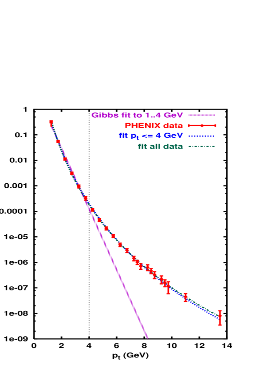
Figure 1: The minimum bias neutral pion $p_{{\mathrm{t}}}$ spectrum from Au-Au collisions at 200 GeV/nucleon from the PHENIX group. Displayed is the spectrum ${\mathrm{d}}N/(2\pi p_{{\mathrm{t}}}{\mathrm{d}}p_{{\mathrm{t}}}{\mathrm{d}}y)$ at $y=0$ as function of the transverse momentum $p_{{\mathrm{t}}}$. Experimental data (large dots with solid error bars) are used in the range 1-4 GeV for fit to BG (dotted straight line) and for Tsallis (dashed curve) distributions, as well as a Tsallis fit over all data points (dash-dotted curve), the latter having $T=118$ MeV, $q=1.1173$. The BG fit is manifestly inadequate, while the two Tsallis functions remain quite close to each other, so the fit in 1-4 GeV yields a surprisingly good prediction for higher energies.

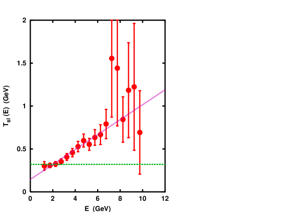
Figure 2: The inverse slope of the neutral pion spectrum for minimum bias as function of $E=m_{{\mathrm{t}}}$. The data (points with solid error bars) are obtained by numerical derivation from the data in Fig. 1, the BG constant at $320$ MeV is a guide to the eye for the low-energy part (horizontal line), and the linear, increasing, function is the Tsallis fit, with $T=165$ MeV and $q=1.094$.

In Fig. 2 we plot the spectral temperature, i.e., the inverse logarithmic slope $T_{{\mathrm{sl}}}(E)$, as defined in eq. (6), obtained from the neutral pion cross section of Fig. 1 by numerical derivation versus the transverse mass $E=m_{t}=\sqrt{(m^{2}+p_{{\mathrm{t}}}^{2})}$. This choice of the energy variable $E$ does not take into account transverse flow corrections. The error bars in $T_{{\mathrm{sl}}}(E)$ were computed from the statistical error in ${\mathrm{d}}N/(2\pi p_{{\mathrm{t}}}{\mathrm{d}}p_{{\mathrm{t}}}{\mathrm{d}}y)$ by assuming Gaussian error propagation. For these data the constant $T_{{\mathrm{sl}}}(E)=T$, that is, the BG distribution, is definitely excluded. The transformed data points do show a monotonous rise, but with a distinct curvature in the low-energy part. Since this is in the flow-sensitive region, and presently flow effects are neglected, it would not make sense to try to reproduce the curve. We give a linear, i.e., Tsallis, fit only for the range $1-7$ GeV, because for higher energies the error is becoming large. The Tsallis fit is compatible with the data points considering the error bars, but the uncertainty of the fit is demonstrated by the difference in the fitted value of the Tsallis temperature $T\approx 165$ MeV from that in Fig. 1. The present fitting is obviously not deciding about the precise shape of $T_{{\mathrm{sl}}}(E)$, however, it shows in tendency a predominantly linear deviation from the assumption of a constant, i.e., BG temperature function.

We tested the consistency of the above fit by separately considering different centrality bins: all $\pi^{0}$ data seem to have been fitted by one $T_{{\mathrm{sl}}}(E)$ curve irrespective of centrality. Therefore we think it made sense to use minimum bias data for a common fit, the more so because that way the statistical errors were better suppressed.

III.2 Flow corrections

Given the importance of the low momentum range for the overall fit, we also have to take into account the transverse flow. First we recapitulate the standard treatment of a collective flow emitting hadrons Csernai (1994). We shall consider differential spectra of hadrons, identified via the rest mass $m$, detected with a certain transverse momentum, $p_{{\mathrm{t}}}$, azimuthal angle $\varphi$ and longitudinal rapidity $y$. The four-momentum of such a hadron is given by

$$p=(m_{{\mathrm{t}}}\cosh y,\>m_{{\mathrm{t}}}\sinh y,\>p_{{\mathrm{t}}}\cos\varphi,\>p_{{\mathrm{t}}}\sin\varphi),$$ (23)

with $m_{{\mathrm{t}}}=\sqrt{m^{2}+p_{{\mathrm{t}}}^{2}}$. Such hadrons may come from different space-time points of an emitting source. The position of the emission is characterized by the four-vector,

$$x=(\tau\cosh\eta,\>\tau\sinh\eta,\>r\cos\psi,\>r\sin\psi).$$ (24)

The total number of detections is described by an eight-dimensional integral of the one-particle phase space density, essentially the Wigner function:

$$N\,=\,\int\!{\mathrm{d}}^{4}x\int\!{\mathrm{d}}^{4}p\,\quad W(x,p).$$ (25)

We adopt here the widespread assumption that the emission of the finally detected hadrons happens at a certain longitudinal proper time, the break-up time $\tau=\tau_{\mathrm{br}}$, but otherwise homogeneously in a cylindrical three-volume, $V=\pi R^{2}L$, with radius $R$ and length $L=2\tau_{\mathrm{br}}\eta_{0}$. Experimental data are available for transverse spectra of identified hadrons, i.e. for

$$\frac{{\mathrm{d}}N^{(m)}}{p_{{\mathrm{t}}}{\mathrm{d}}p_{{\mathrm{t}}}{\mathrm{d}}\varphi{\mathrm{d}}y}\,=\,mV\int_{-\eta_{0}}^{\eta_{0}}\frac{{\mathrm{d}}\eta}{2\eta_{0}}\int_{-\pi}^{\pi}\frac{{\mathrm{d}}\psi}{2\pi}\,f(E),$$ (26)

where the energy distribution $f(E)$ is the thermodynamical distribution we are seeking to learn about. The energy-variable, $E$, in this distribution is the energy in the local Lorentz frame, $E=u\cdot p$, with $u$ being the four-velocity of the emitting cell. (In the case $f(E)$ is the BG distribution, this version is called the Jüttner distribution.)

A further simplifying assumption is to consider a scaling longitudinal flow (the so called Bjørken flow) combined with a transverse radial expansion of velocity $v$. The four-velocity becomes

$$u\,=\,(\gamma\cosh\eta,\>\gamma\sinh\eta,\>\gamma\,v\cos\varphi,\>\gamma\,v\sin\varphi)$$ (27)

with $\gamma=1/\sqrt{1-v^{2}}$. In this case

$$E\,=\,\gamma\,m_{{\mathrm{t}}}\cosh(y-\eta)\>-\>\gamma\,v\,p_{{\mathrm{t}}}\cos(\varphi-\psi).$$ (28)

According to eq. (26) the detectors see an average of the local thermodynamical distribution over $\eta$ and $\psi$. This integral can be calculated analytically for the BG distribution resulting in a product of the $K_{0}(\gamma m_{{\mathrm{t}}})$ and $I_{0}(\gamma vp_{{\mathrm{t}}})$ Bessel functions, but it is not so in the Tsallis or in more general cases. Numerical integration is doable by using suitable ansätze for $f(E)$, but then one looses the possibility of direct reconstruction of this function from observational data. Another way is to make yet further simplifying assumptions on the emitting source, but keeping a general $f(E)$.

Following the second reasoning we adopt the physical picture that the main contribution to the detected spectrum is due to forward emission, that is, it comes from those particles that fly in the same direction as the emitting volume element. Thus we replace the $E$ function by its value at $\eta=y$ and $\psi=\varphi$, i.e., $E=\gamma(m_{{\mathrm{t}}}-vp_{{\mathrm{t}}})$. We learn that the shape of the observed transverse distributions at large $p_{{\mathrm{t}}}$ is effected only by an overall blue-shift, $p_{{\mathrm{t}}}=E\sqrt{\frac{1+v}{1-v}}$ , while at small $p_{{\mathrm{t}}}$ mass-dependent effects occur. For instance, in the non-relativistic limit $f(E(p))$ is Gaussian in $p_{{\mathrm{t}}}$ such that the variance depends on the rest mass as $\langle p_{{\mathrm{t}}}^{2}\rangle=mT^{\ast}=m(T_{0}+mv^{2})$, where $T^{\ast}$ is the empirical temperature and $T_{0}=T_{{\mathrm{sl}}}(E=m)$ is the local inverse slope at rest. This picture is in general accordance with the widely accepted role of the hydrodynamical flow on the particle spectrum.

Fig. 3 shows the inverse logarithmic slope, $T_{{\mathrm{sl}}}(E)$ extracted from antiproton, negative kaon and pion, and neutral pion data from Adler et al. (2004) with the assumption $E=\gamma(m_{{\mathrm{t}}}-vp_{{\mathrm{t}}})$. The curves for different hadron types fit so well together with a common $v=0.5$ that this strongly supports the assumption about the statistical origin of the local $f(E)$ distribution. A faster transverse flow, e.g. $v=0.6$ already overcompensates the low-$p_{{\mathrm{t}}}$ data for antiprotons turning the temperature $T_{{\mathrm{sl}}}(E)$ abruptly down towards negative values, therefore we stick with the maximal flow value of $v=0.5$ not showing the downturn. The Tsallis fits, which may be layed on the data are not fine enough; a surprisingly low temperature parameter and a relatively high deviation from the BG distribution with $T=20.5$ MeV and $q=1.26$ (Tsallis fit 1) goes through the data points with error bars as well as the Tsallis fit 2 with $T=113$ MeV and $q=1.081$. In the latter case at the lowest $p_{\mathrm{t}}$ data the virtual slope is $T_{{\mathrm{sl}}}(0.825GeV)=165.5$ MeV, roughly equal to the conventional BG estimate.

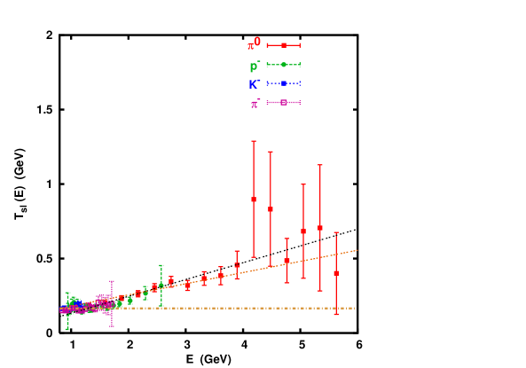
Figure 3: Inverse logarithmic slopes obtained from transverse flow corrected $p_{{\mathrm{t}}}$ spectra of various particles. The flow corrected energy $E=\gamma(m_{\mathrm{t}}-vp_{\mathrm{t}})$ is on the horizontal axis, while $T_{\mathrm{sl}}(E)={\mathrm{d}}E/{\mathrm{d}}m_{\mathrm{t}}\,T_{\mathrm{sl}}(m_{\mathrm{t}})=\gamma(1-vm_{\mathrm{t}}/p_{\mathrm{t}})\,T_{\mathrm{sl}}(m_{\mathrm{t}})$ on the vertical one, where $T_{\mathrm{sl}}(m_{t})=-f/({\mathrm{d}}f/{\mathrm{d}}m_{\mathrm{t}})$, and $f(m_{t})$ were taken from the experiments. The particle data $\pi^{0}$ (squares with solid error bars), antiprotons (large dots with dashed bars), $K^{-}$ (squares with short dashed bars), $\pi^{-}$ (open squares with dotted bars) were fitted with a common $v=0.5$ to two Tsallis linear functions, (1) with $T=20.5$ MeV and $q=1.26$ (short dashed lines grouped in two) and (2) with $T=113$ MeV and $q=1.081$ (short dashed lines grouped in three). The BG line (dash-dotted) is horizontal, obtained from a fit for $E<1.5$ GeV.

It is clear, however, that more work is needed to go beyond our crude estimate of the flow’s effect, possibly in an iterative manner with ever better approximations for the stationary distribution. On the other hand, since higher $p_{{\mathrm{t}}}$ data at RHIC are expected, we are looking forward to learn more about a possibly non-BG behavior in a momentum range where transverse flow effects little distort the local slope in particle spectra.

IV Conclusion

In this paper we considered generalized stationary energy distributions in the case of energy dependent damping and noise. We have shown that the BG and Tsallis distribution are the most simple particular cases of this framework. As a physical example, high energy transverse momentum distributions have been analyzed from relativistic heavy ion experiments at RHIC. The high energy part of the neutral pion data (above $p_{{\mathrm{t}}}\approx 2-4$ GeV) excludes the Boltzmann-Gibbs distribution. This fact earlier has been interpreted as a sign for a non-equilibrium component in the spectra Fries et al. (2003a, b). Recent field theoretical model estimates on the speed of thermalization, however, predict at least partial equilibration, called “prethermalization” Sexty and Patkós . According to our ideas presented in this paper, a generalized equilibrium interpretation of these spectra becomes thinkable. Finally we note that the best fit to the data, while definitely excludes the BG distribution, at this stage does not decisively support the Tsallis distribution either. A more general distribution based on a quadratic energy dependence of the diffusion coefficient is also a possible interpretation. In this respect further investigations are needed to clarify the deformation effect of transverse flow on the discussed spectra. Higher particle yields are also desirable because they can lead to narrowing error bars for larger energies.

Finally we stress that our empirical findings are reminiscent to the result reported about by Walton and Rafelski Walton and Rafelski (2000) on charmed quark emission, where a predominantly linear $T_{{\mathrm{sl}}}(E)$ has been obtained from perturbative QCD, albeit with a slight curvature. This raises the hope for a theory that describes microscopically the quark-gluon-plasma, produces a foundation for the Fokker-Planck approach and connects it to the detected spectra.