Does Reactor Neutrino Experiment Play an Important Role in $\theta_{13}$ of Lepton Mixing (PMNS) Matrix ?

Abstract

Reactor neutrinos play an important role in determining parameter $\theta_{13}$ in the lepton mixing (PMNS) matrix. A next important step on measuring PMNS matrix could be to build another reactor neutrino experiment, for example, DaYa Bay in China, to search the possible oscillations via $\sin^{2}2\theta_{13}$ and $\Delta m^{2}_{13}$. We consider 4 different schemes for positions of three 8-ton detectors of this experiment, and simulate the results with respect to an array of assumed ”true” values of physics parameters. Using three kinds of analysis methods, we suggest a best scheme for this experiment which is to place a detector $2200m\sim 2500m$ symmetrically away from two reactors, and to put the other two detectors closer to their corresponding reactors respectively, almost at a $100m\sim 200m$ distance. Moreover, with conservative assumption on the experimental technique, we construct series of allowed regions from our simulation results, and give detailed explanations therein.

I Introduction

An next step in the exciting field of neutrino physics would be to improve current measurements and to measure some of the remaining unknown parameters in the full $3\times 3$ leptonic flavor mixing, which is called the PMNS mixing matrix. There are important differences between the PMNS and quark CKM matrices. Which may be essential for our understanding the underlying physics. In addition to three masses $m_{i}$, there are 6 free parameters in the matrix. We may parameterize $U_{PMNS}$ [1] as follows:

$$U_{PMNS}=U_{12}\times U_{23}\times U_{13}\times U_{major}.$$ (1.1)

$$U_{12} = \left(\begin{array}[]{ccc}\cos\theta_{12}&\sin\theta_{12}&0\\ -\sin\theta_{12}&\cos\theta_{12}&0\\ 0&0&1\end{array}\right)$$ (1.5)

$$U_{23} = \left(\begin{array}[]{ccc}1&0&0\\ 0&\cos\theta_{23}&\sin\theta_{23}\\ 0&-\sin\theta_{23}&\cos\theta_{23}\end{array}\right)$$ (1.9)

$$U_{13} = \left(\begin{array}[]{ccc}\cos\theta_{13}&0&e^{-i\delta_{CP}}\sin\theta_{13}\\ 0&1&0\\ -e^{-i\delta_{CP}}\sin\theta_{13}&0&\cos\theta_{13}\end{array}\right)$$ (1.13)

$$U_{major} = \left(\begin{array}[]{ccc}1&0&0\\ 0&e^{-i\alpha}&0\\ 0&0&e^{-i\beta}\end{array}\right)$$ (1.17)

$U_{23}$ and the value of $\Delta m_{23}^{2}$ have been measured by the Super-Kamiokande [2] and K2K long base line experiments [3]; while $U_{12}$ and the value of $\Delta m_{12}^{2}$ are parameters of the confirmed solar neutrino MSW [4] solution. $U_{major}$ is the possible majorana phase matrix, its values and the overall mass scale will require kinematical and neutrino-less double-$\beta$ decay measurements. $U_{13}$ is the next goal for the experiments since it will tell us, in particular, if $CP$ violation is possible in the lepton sector. We can expect it from the very long base line experiments such as JPARC, H2B [5, 6] and, new generation of reactor neutrino experiments.

The CHOOZ experiment [7, 8] only gives an upper limit on the mixing angle $\theta_{13}$ ($\sin^{2}2\theta_{13}<0.10$ at $90\%$ confidence level). There are attempts to find this mixing angle in LBL accelerator experiments [5, 6], or in three neutrino analysis of solar neutrino [6, 9, 10], but the precision is very difficult to achieve. Since $\Delta m_{12}^{2}\ll\Delta m_{23}^{2}$, it must happen that $\Delta m_{13}^{2}\approx\Delta m_{23}^{2}$. A new generation of reactor experiments has been proposed to search for $\bar{\nu}_{e}$ disappearance at baselines of  1 $\sim$ 2 km corresponding to this value of $\Delta m^{2}$. To improve on the mixing angle sensitivity achieved by Palo Verde and CHOOZ, proposals for reactor $\theta_{13}$ experiments include a large detector to reduce the statistical error, and also a second detector positioned very close ($\sim$ 100 m) to the reactor. The near detector would precisely measure the incident flux, providing to drop out many systematic uncertainties in the flux calculation. This also requires the detectors to be made identical and/or movable. Sensitivity down to $\sin^{2}2\theta_{13}\approx 10^{-2}$ seems within grasp. Such experiments were discussed in literature [11, 12]. A practical possibility is a reactor experiment at DaYa-Bay, which is located near a special economic zone in Guang-Dong Province in southern China. There are nuclear power plants in that area.

The knowledge we have about neutrino mixing is powerful to judge Grand Unified models, such as the most inspiring SO(10) GUT. Starting from the lepton quark symmetry in this model, one is able to obtain a bi-large neutrino mixing pattern via see-saw mechanism. It leads to a non-zero $\sin^{2}2\theta_{13}$, e.g., at about $0.09$ in paper [13], which is out of CHOOZ’s limit but is very easy to discover in DaYa-Bay experiment within one year operation.

In this paper we will describe the importance of reactor neutrinos in determination of $\sin^{2}2\theta_{13}$ - $\Delta m^{2}_{13}$; we will concentrate on possible new China experiment and its goal - finding $\sin^{2}2\theta_{13}$. The paper is organized as follows: first, we will describe a possible reactor experiment in DaYa-Bay (see fig. 1), which is a kind of upgraded CHOOZ experiment[11, 14, 15]; its possible systematic and statistical uncertainties are analogies to the CHOOZ’s one. Next we will explain different methods of analysis, and importantly, our arrangement of the detectors’ positions, accompanied by our simplified Monte Carlo simulations on the possible sensitivity regions for $\sin^{2}2\theta_{13}$; and discovery potentialities are discussed therein. Finally, we will give our conclusion of the paper.

II Reactor Neutrinos

In a reactor, anti-neutrinos are released by radioactive isotope fission; the total neutrino spectrum is a rather well understood function of the thermal power $W$, the amount of thermal power $w_{i}$ emitted during the fission of a given nucleus, and the isotopic composition of the reactor fuel $f_{i}$,

$$S(E_{\nu})=\frac{W}{\sum f_{i}w_{i}}\sum f_{i}\left(\frac{dN}{dE_{\nu}}\right)_{i}$$ (2.1)

The index $i$ of $f_{i}$ stands for 4 isotopes such as ${}^{235}U$, ${}^{238}U$, ${}^{239}Pu$ and ${}^{241}Pu.$ The (dN/dE) is the energy spectrum of the fissionable isotope, it can be parameterized by the following expression[16] when $E_{\nu}\geq$ $2MeV$:

$$\frac{dN_{\nu}}{dE_{\nu}}=e^{a_{0}+a_{1}E_{\nu}+a_{2}E_{\nu}^{2}}$$ (2.2)

the coefficients $a_{i}$ depend on the nature of the fissionable isotope. KamLAND is a scintillator detector, where electronic anti-neutrinos are detected by free protons via inverse $\beta-$decay reaction[16],

$$\overline{\nu}_{e}+p\rightarrow e^{+}+n$$ (2.3)

In the limit of infinite nucleon mass, the cross section of this reaction is given by $\sigma(E_{\nu})=kE_{e^{+}}P_{e^{+}}$, where $E_{e^{+}},~{}P_{e^{+}}$ are the positron energy and momentum respectively and $k$ can be taken as $k=9.55\times 10^{-44}~{}cm^{2}/MeV^{2}$. The anti-neutrino events are characterized by the positron annihilation signal and the delayed neutron capture sign [17].

From the reactor to the detector, massive neutrinos oscillate on the way and change their flavor composition to a certain extent. The anti-neutrino $\overline{\nu}_{e}$ can oscillate to other flavors via $\Delta m_{12}^{2}$ and $\Delta m_{13}^{2}$. In principle, reactor neutrinos are able to give us information about $\Delta m_{13}^{2}$ $\&$ $\Delta m_{12}^{2}$ and two mixing angles $\sin^{2}2\theta_{13}$ $\&$ $\sin^{2}2\theta_{12}$, which are almost all the neutrino oscillation parameters except $\sin^{2}2\theta_{23}$. This advantage of reactor neutrinos is due to its low energy, which is several MeV, comparing with accelerator neutrinos’ GeVs. Reactor experiment like DaYa Bay is sensitive to $\sin^{2}2\theta_{13}$ and $\Delta m_{13}^{2}$. This is the second order oscillating effect of the reactor neutrinos, comparing with the oscillations induced by $\theta_{12}$ and $\Delta m_{12}^{2}$. Since the energy of detectable reactor neutrino is about MeVs, from atmospheric oscillation experiments, $\Delta m_{13}^{2}$ is in the range of $1.3\sim 5.0\times 10^{-3}\mathtt{eV}^{2}$ at $99\%$C.L. [2], with the best fitted point $2.5\times 10^{-3}\mathtt{eV}^{2}$, so the expected maximum oscillation is reached at about 1500 m. Then the survival probability is reduced to the two flavor neutrino case:

$$P(E_{\nu},L,\theta_{13},\Delta m_{13}^{2})=1-\sin^{2}(2\theta_{13})\sin^{2}\left(\frac{1.27\Delta m_{13}^{2}(\mathtt{eV}^{2})L(\mathtt{m})}{E_{\nu}(\mathtt{MeV})}\right)$$ (2.4)

where $\sin^{2}2\theta_{13}$ is the only unknown parameter here, which is our major interest in this paper.

III Possible
Reactor Neutrino Experiment in China

DaYa-Bay is one of the Chinese running reactor power plants, located in Guang-Dong province, south China, and it is quite close to Hong Kong. The DaYa Bay nuclear power plant consists of two twin reactor cores, separated about $1200$ m from each other, one is called DaYa, the other is called LingAo, each core can generate a thermal power of $2.9$ $GW$, making a total of $11.6$ $GW$, and a third twin core is planned to be on line in 2010. The reactors are built near a mountain, so it is possible to build a near experiment hall with an overburden of $400$ $mwe$ at a distance of about $300$ $m$ to the core and a far hall with an overburden of $1200$ $mwe$ at a distance of about $1500\sim 2000$ $m$ to the core. This is a certain improvement in comparison with the CHOOZ experiment which has a value of $8.5$ $GW$ in thermal power, and $300$ $mwe$ in rock overburden.

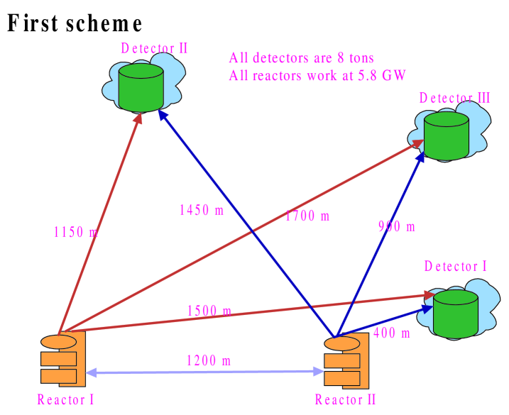
Figure 4: First scheme: we arrange three detectors in distances from the reactors in the range of $400m\sim 1700m$ unsymmetrically.

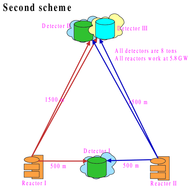
Figure 5: Second experiment scheme: three detectors are placed symmetrically according to two reactors, one is on the middle points, the other two are superposed on the perpendicular bisector equidistant 1500m from the two reactors.

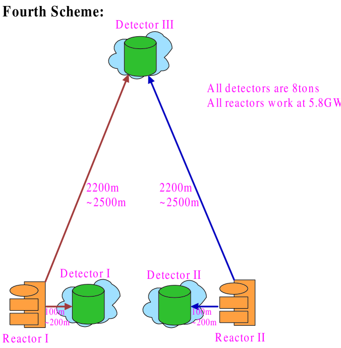
Figure 7: Fourth scheme: similar to scheme 3, but two near detectors are put on the line between two reactors; and the distance of the far detector is enlarged to $2200\sim 2500$ $m$.

Three liquid scintillation calorimeter detectors can be placed from distances between several hundreds meters (near detectors) to about $2$ $km$ (far detectors) from the cores as shown in figs. 4 - 7. High intensity and purity electron anti-neutrino flux from the reactor core is detected via the inverse beta-decay reaction eq. (2.3), the signature is a delayed coincidence between the prompt $e^{+}$ signal and the signal from the neutron capture, the target material can be the Hydrogen-rich (free protons) paraffin-based liquid scintillator loaded with Gadolinium, which is chosen due to its large neutron capture cross section and to the high $\gamma$-ray energy released after $n-$capture. The rock overburdens are able to reduce the external cosmic ray muon flux by a fact of more than 300. To protect the detector from natural radioactivity of the rock, the steel vessel should be surrounded by $\sim 100cm$ of low radioactivity sand and covered by $\sim 15cm$ of cast iron. There are three concentric regions in a detector: as shown in fig. 2: one is a central 8 tons working target in a transparent Plexiglas container filled with a $0.09\%$ Gd-loaded scintillator; the second should be an intermediate region, equipped with hundreds eight-inch PMT’s, used to protect the target from PMT radioactivity and to contain the gamma rays from neutron capture; the third can be an outer optically separated active cosmic-ray muon veto shield equipped with two rings of tens eight-inch PMT’s. All these arrangements could significantly decrease the most dangerous background. Moreover, the particular coincidence between the prompt positron signal and the delayed neutron capture signal could significantly reduce the accidental background. Rates from background can be suppressed down to $0.2\thicksim 0.3$ events per day per ton, which corresponds to more than $60\%$ of a detection efficiency.

Besides the uncertainty in the efficiency, there are other uncertainties contained in the experiment: the reaction cross section uncertainty from an overall and conservative uncertainty on integral neutrino rate, $1.9\%$; the number of target protons uncertainty ($0.8\%$), mainly because of the difficulty in determining the hydrogen content; the overall precision on the thermal power is claimed to be $0.7\%$; the uncertainty of the average energy released per fission of the main fissile isotopes is $0.6\%$. The five uncertainties presented above are all overall effective, and we could combine them to a total effect with a value of $2.7\%$. However, as the uncertainty of the energy scale ($1.1\%$) affects the experimental result varying with respect to the energy bins, we have to specially consider its influence.

It is supposed that only one of the two nucleon power plants would run for the most of the total time of the experiment. This allow us to know from which reactor the signal is generated. Otherwise, the detector should be desired to be able to distinguish the events induced by the first reactor binary-core from the other. In the paper [18], a good determination of the anti-neutrino incoming direction is discussed. It is based on the neutron boost in the forward direction via the inverse beta-decay reaction, which is induced by the incident neutrino; the kinetic energy of the neutron remains even after collisions with protons inside the detector.

IV Three methods of Analysis

Let us suppose that the experiment like DaYa-Bay will measure the positron spectrum in 7 bins (from $E_{1}$ to $E_{7})$. For a mean reactor-detector distance $L_{k}$, the rates can be written as

$$S_{k}(E,L_{k},\theta,\Delta m^{2})=\frac{N_{p}}{4\pi L_{k}^{2}}\int h(L,L_{k})\int\sigma(E_{\nu})S(E_{\nu})P(E_{\nu},L,\theta,\Delta m^{2})r(E_{e^{+}},E)\varepsilon(E_{e^{+}})dE_{\nu}dE_{e^{+}}dL$$ (4.1)

where

$E_{\nu},E_{e^{+}}$	are neutrino energy and positron energy respectively,
$N_{p}$	is the total number of target protons
	in the Region I scintillator,
$\sigma(E_{\nu})$	is the detection cross section,
$S(E_{\nu})$	is the anti-neutrino spectrum,
$h(L,L_{k})$	is the spatial distribution function for
	the finite core and detector sizes,
$r(E_{e^{+}},E)$	is the detector response function linking
	the visible energy $E$ and the real positron energy$E_{e^{+}}$
$P(E_{\nu},L,\theta,\Delta~{}m^{2})$	is the two-flavor survival probability,
$\varepsilon(E_{e^{+}})$	is the neutrino detection efficiency.

The fissile isotope composition varies with respect to the working time, because the 4 isotopes burn a bit differently. The expected number of neutrino is a function of working time, reactor power and a constant background.

$$N_{i}^{j}=(B^{j}+W_{1j}\cdot Y_{1i}^{j}+W_{2i}\cdot Y_{2i}^{j})\cdot\Delta t_{i}$$ (4.2)

where the index $i$ labels the run number or the working time information; $\Delta t_{i}$ is the corresponding live time interval; $j$ labels the detector number; $B^{j}$ is the background rate, which is assumed to be a constant with time in our study; ($W_{1i}$, $W_{2i}$) are the thermal powers of the two binary-core reactors in GW and ($Y_{1i}$, $Y_{2i}$) are the positron yields per GW per day induced by each reactor. Since we are considering several detectors, it is convenient to factorize $Y_{ki}^{j}$ and $B^{j}$ into functions which separate the factors which are independent of the detectors’ size:

$$Y_{ki}^{j}=(1+\eta_{ki}^{j})\cdot\frac{(1~{}km)^{2}}{(L_{k}^{j})^{2}}\cdot X_{k}^{j}\cdot T^{j},$$ (4.3)

$$B_{i}^{j}=b_{i}^{j}\cdot T^{j},$$ (4.4)

where $k=1,2$ is the index of the reactors, associated with $T^{j}$ tons of available detector material, $\eta_{ki}^{j}$ stands for corrections from the reactor’s differences on the fissile isotope composition and the positron efficiency correction. The complications varying with time are all involved in $\eta_{ki}^{j}$; this effect will be considered in real measurement and will not be taken into account in our simulations. $X_{k}^{j}$ represent the positron events contribution in $1$ ton fresh detective material from a fresh reactor located 1km away, with its thermal power equal to 1GW within one day. In the following we compare the two positron spectra $X_{k}^{j}$ which are the measured one and the oscillation expected one. It can be parameterized by separating the oscillation term from the no-oscillation one:

$$X_{k}^{j}(E_{l},L_{k}^{j},\theta,\Delta m_{13}^{2})=X_{0}(E_{l})\overline{P}(E_{l},L_{k}^{j},\theta,\Delta m_{13}^{2}),$$ (4.5)

where $X_{0}(E_{l})$ is the no-oscillation positron spectrum, unitary for all the detectors in our definition, and $E_{l}$ label the visible energy bins:

$$X_{0}(E_{l})=\frac{n_{p}}{4\pi(1~{}km)^{2}}\int\sigma(E_{\nu})S(E_{\nu})\int r(E_{e^{+}},E)\varepsilon(E_{e^{+}})dE_{e^{+}}dE_{\nu}$$ (4.6)

and $\overline{P}$ is the survival probability averaged over the energy bins and the finite sizes of both the detector and the reactor core,

$$\overline{P}(E_{l},L_{k}^{j},\theta,\Delta m^{2})=\frac{\int S_{k}(E,L_{k}^{j},\theta,\Delta m^{2})dE}{\int S_{k}(E,L_{k}^{j},0,0)dE}$$ (4.7)

With these definitions, we can begin to investigate our detector systems’ power. In the reactor neutrino oscillation experiment like DaYa-Bay, we suggest that several detectors located at different places have no difference between them, which means they have a same design; thus the systematic uncertainties are supposed to be the same in order to cancel out some negative effects by comparison. In this paper, without losing generality, we suppose that: three detectors have 8 tons of Gd-loaded scintillator each; two nuclear reactors each working at 5.8GW of its full thermal power.

To test an oscillation hypothesis ($\Delta m^{2}$, $\sin^{2}2\theta$) in our experiment, we construct a $\chi^{2}$ function including the 6 positron spectra measured and the oscillation expected in a 42-element X array, as follows:

$${\overrightarrow{X}=(\overrightarrow{X_{1}^{1}},\overrightarrow{X_{1}^{2}},\overrightarrow{X_{1}^{3}},\overrightarrow{X_{2}^{1}},\overrightarrow{X_{2}^{2}},\overrightarrow{X_{2}^{3}})},$$ (4.8)

$$\overrightarrow{X_{i}^{j}}=(X_{i}^{j}(E_{1}),X_{i}^{j}(E_{2}),X_{i}^{j}(E_{3}),X_{i}^{j}(E_{4}),X_{i}^{j}(E_{5}),X_{i}^{j}(E_{6}),X_{i}^{j}(E_{7})),$$ (4.9)

where the subscript $i$ is the reactor’s number, and the superscript $j$ is the detector’s number. Combining the statistical variances with the systematic uncertainties related to the neutrino spectra, the $42\times 42$ covariance matrix can be written in a compact form as follows:

$$V_{ij}=\delta_{i,j}(\sigma_{i}^{2}+\widetilde{\sigma_{i}}^{2})+(\delta_{i,j-21}+\delta_{i,j+21})\cdot\sigma_{12}^{(i)},~{}~{}(i,j=1,\cdot\cdot\cdot 42)$$ (4.10)

where $\sigma_{i}$ are the statistical errors, $\widetilde{\sigma_{i}}$ are the corresponding systematic uncertainties, and $\sigma_{12}^{(i)}$ are the statistical covariance of the reactor 1 and 2 yield contributions to the $i$-th measurement.

A.

There are two kinds of uncertainties influencing all the measurements which can’t be ignored, the overall normalization uncertainty which is $\sigma_{a}\thickapprox 2.7\%$, and the spectrum affective energy-scale calibration uncertainty which is $\sigma_{g}=1.1\%$. We consider these two as in eq. (4.11) to reach the minimum $\chi_{A}^{2}$ for a set of proposed oscillation parameters:

$$\chi_{A}^{2}(\theta,\Delta m^{2}) = \min_{a,g}\left[\sum_{i,j}(\hat{X}^{i}-a\cdot\overline{\hat{X}}^{i}(gE,\theta,\Delta m^{2}))\left(V^{-1}\right)_{i,j}(\hat{X}^{j}-a\cdot\overline{\hat{X}}^{j}(gE,\theta,\Delta m^{2}))\right.$$ (4.11)

$$\left.+\left(\frac{a-1}{\sigma_{a}}\right)^{2}+\left(\frac{g-1}{\sigma_{g}}\right)^{2}\right],$$

where $\hat{X}^{i}$ stands for measured or simulated one, and $\overline{\hat{X}}^{i}(gE,\theta,\Delta m^{2})$ for oscillation expected one. Here we have taken into account the statistic uncertainty, so we add up a hat on $X^{i}$. The statistic error is the square root of the event number which depends on the detector size, the reactor power and the experiment’s life time. This method uses all the experimental information available, and directly depends on the correct determination of the systematic uncertainties. Such uncertainties could be reduced by measuring the positron spectrum with a detector near the reactors. When a product of the reactor power, the detector size and the working time is large enough to reduce the statistical uncertainty, we could constrain this overall normalization coefficient and the energy-scale calibration precisely.

B.

We compare the ratio of the two reactors’ contribution in another way. Since the expected spectra are the same for both reactors in the case of no-oscillation, the ratio reduces to the ratio of the average survival probabilities. Detectors are assumed to be the same, the systematic uncertainties will be canceled out or almost canceled out and the remaining uncertainty we should take into account is just the statistical uncertainty. So we can construct $\chi^{2}_{B}$ by

$$R^{j}_{k}=\frac{\hat{X}^{j}_{1}(E_{k})}{\hat{X}^{j}_{2}(E_{k})},~{}~{}~{}~{}~{}~{}\delta R^{j}_{k}=R^{j}_{k}\cdot\left(\frac{\delta\hat{X}^{j}_{1}(E_{k})}{\hat{X}^{j}_{1}(E_{k})}+\frac{\delta\hat{X}^{j}_{2}(E_{k})}{\hat{X}^{j}_{2}(E_{k})}\right),$$

$$\chi^{2}_{B}(\theta,\Delta m^{2})=\sum_{j,k}\left(\frac{R^{j}_{k}-R^{j}_{k}(\theta,\Delta m^{2})}{\delta R^{j}_{k}}\right)^{2}$$ (4.12)

$\chi_{B}^{2}$ is a good quantity to judge an oscillation result from no-oscillation one in the case where the distances to every reactor for a detector are quite different. In the CHOOZ experiment the distance difference is just $116.7$ $m$, so that the $\chi_{B}^{2}$ is less powerful than $\chi_{A}^{2}$ [7]. In our experiment design, the near detectors are expected to be placed at positions which give a larger distance difference; thus we can expect $\chi_{B}^{2}$ is more powerful.

C.

There is an intermediate analysis approach between the $\chi_{A}^{2}$ and $\chi_{B}^{2}$. It uses the shape of the positron spectrum, while leaving the absolute normalization free. Similar to approach A, this approach fits the two uncertainties, but leaving the normalization parameter unconstrained, that is:

$$\chi_{C}^{2}(\theta,\Delta m^{2})=\min_{a,g}\left[\sum(\hat{X}^{i}-a\cdot\overline{\hat{X}}^{i}(gE,\theta,\Delta m^{2}))\left(V^{-1}\right)_{i,j}(\hat{X}^{j}-a\cdot\overline{\hat{X}}^{j}(gE,\theta,\Delta m^{2}))+\left(\frac{g-1}{\sigma_{g}}\right)^{2}\right]$$

In the following, we will use these three analysis methods to constrain the oscillation parameters for the possible reactors and detectors systems. With these results, we are able to judge which kind of system and the corresponding approach is the most powerful one.

V Examining Arrangements and Simulation Results

Comparing with the CHOOZ experiment, DaYa-Bay has more powerful reactors, longer working time, more larger detectors. Let us suppose the nuclear power plants work at its full thermal power 5.8(GW), the detector’s available mass is 8 tons, and the experiment life time is set to be one year in our first simulation. We assume we had known the signal’s corresponding reactor individually.

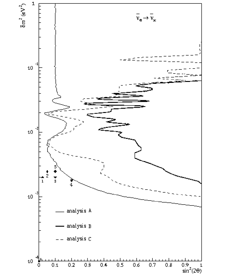
Figure 3: Six points whose coordinates are considered as real physics parameters for the first 3 schemes’ simulations, in CHOOZ’s excluded region. First ponit represents no-oscillation, labelled as “0”. The other five points below will cause oscillation effect; their parameters ($\sin^{2}2\theta_{13}$, $\Delta m^{2}$ [eV²] ) are 1$\rightarrow$(0.02, $2.0\times 10^{-3}$), 2$\rightarrow$(0.05, $2.5\times 10^{-3}$), 3$\rightarrow$(0.1, $2.0\times 10^{-3}$), 4$\rightarrow$(0.2, $1.7\times 10^{-3}$), 5$\rightarrow$(0.1, $2.5\times 10^{-3}$).

1) In our first scheme, three detectors with distances from the reactors in the range of $400m\sim 1700m$ are arranged asymmetrically as plotted in fig. 4. Every detector can give two different distances with its corresponding oscillation spectra. This scheme is based on an idea: the allowed region of $\Delta m^{2}$ ($=\Delta m_{atm}^{2})$ given by the atmospheric data is still too big to determine the best position for all detectors; in order to consider all the possible $\Delta m^{2}$, we try to place the detectors at different positions which can provide more numbers of different distances. We test our system with some possible parameters chosen from the CHOOZ’s indistinguishable region; the points in that parameter region are shown in fig. 3. We simulate the experiment by using the values of those points one by one as the values of true physics parameters. Like in previous discussions, we assume each possible oscillation hypothesis to construct the excluded/allowed region at different confidence levels [19].

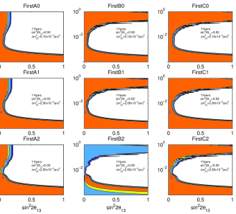
Figure 8: The allowed regions at different confidence levels for the first scheme. The labels “First”, “Second”, “Third” stand for different schemes; “A”, “B”, “C” for different analysis methods, and “0 $\sim$ 2” for the simulation input parameters with their value presented in the figure, in a plot, it is denoted by a plus sign. From this point to the exclusion area, the confidence levels of the four regions are $90\%,95\%,99\%,99.73\%$.

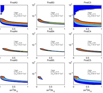
Figure 9: Continue plots of fig. 8

The Monte Carlo simulation results are presented in figs. 8, 9, using three analysis approaches for the six representational possible ”true value” points as signed in fig. 3. For our first detectors’ arrangement, we can see that approach B is the most powerful one while A is less sensitive and C is the lowest. In the following discussion, we will not present our approach C results since A is similar and better. Using analysis approach B in First scheme, the experiment like DaYa-Bay is able to find an oscillation result for $\sin^{2}2\theta_{13}$ bigger than 0.05 (at more than $90\%$ C.L. ), if $\Delta m_{23}^{2}$ is at the region of $\sim~{}2.5\times 10^{-3}\mathtt{eV}^{2}$; and the oscillation parameters can be even constrained to a small allowed region (fig. 9) for bigger $\sin^{2}2\theta_{13}$ (as the last three points we simulated with). It is interesting that one can bound $\sin^{2}2\theta_{13}$ to be bigger than 0.05 at $95\%$ C.L., if the true parameter is located near the point ($\sin^{2}2\theta_{13}=0.1$, $\Delta m^{2}=2.0\times 10^{-3}$eV²); and the best restriction on $\sin^{2}2\theta_{13}$ is reached when the simulated parameters is located near ($\sin^{2}2\theta_{13}=0.1$, $\Delta m^{2}=2.5\times 10^{-3}$eV²); there we could use this system combined with analysis B to constrain the oscillation mixing angle and the mass square difference to a precise region as we present in the subplot (3rd row, 2nd column) named as ’FirstB5’ of fig. 9.

2) In the second scheme[20], fig. 5, the three detectors are arranged symmetrically from the reactors, one is in the middle of two reactors, the other two are superposed on the perpendicular bisector equidistant 1500m from the two reactors. Since the two reactors are symmetric to every detector, approach B is disabled. Approach A can also distinguish $\sin^{2}2\theta_{13}$ bigger than 0.05 if $\Delta m_{23}^{2}$ is near $2.5\times 10^{-3}eV^{2}$; but it can only constrain $sin^{2}2\theta_{13}$ at $95\%$ C.L. and the maximum mixing is not excluded at $99\%$ C.L. even at the most sensitive oscillation points, if by the DaYa-Bay experiment itself.

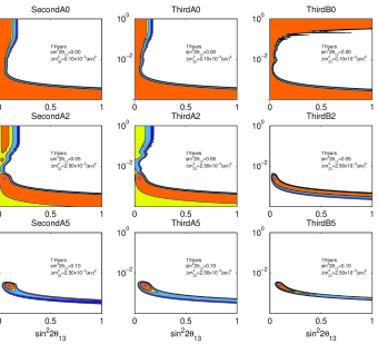
Figure 10: The allowed regions (shadows) of our simulation for second and third schemes, same notations as previous plots.

3) In the third scheme [20], fig. 6, detectors are also disposed symmetrically, but from the near detectors, the two reactors are not equidistant, so the analysis approach B is partly available. For one year’s operation of the experiment, this scheme shows a very clear oscillation signal for $\sin^{2}2\theta_{13}$ larger than $0.05$ at 99.73$\%$ C.L. (2nd row, 3rd column in fig. 10).

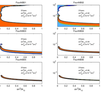
Figure 11: Similar to previous figures, these are results for the Fourth scheme with 3 years’ experiment. The title ”FourthB0x” stands for $\chi^{2}_{B}$ analysis of the simulation with the parameters in the figure.

4) Scheme three is quite good since it gives a higher confidence level than First and Second schemes if there is a positive result for a non zero $\sin^{2}2\theta_{13}$. However it is still possible to improve it. As a conclusion, in this paper, for detectors’ locations, we suggest a possible setting for the experiment like DaYa-Bay, which is called the Fourth scheme: an extension of the Third scheme, which is to put a 8-ton detector $2200m\sim 2500m$ symmetrically away from two reactors; and put the other two 8-ton detectors more close to their corresponding reactors respectively, almost at a $100m\sim 200m$ distance; they are located on the line between the two reactors (see fig. 7). The reason for a $2200m\sim 2500m$-detector is based on the most sensitive oscillation zone with respect to the range of present $\Delta m^{2}_{31}$, taking into account the whole energy spectrum effect of reactor neutrinos. The best way for the two near detectors to easily distinguish which reactor a neutrino signal comes from, is to put the other two detectors on the inner line between two reactors; thus two different neutrino sources are from two opposite directions. We use the $\chi^{2}_{B}$ method to analyze Monte Carlo results, in which the far detector’s data is not taken into account since this detector is symmetric to two reactors; this doesn’t affect our major statement about the discovery potential of this experiment. However, the far detector is important in a real data analysis: using the single $\chi^{2}_{A}$ method it will exclude big-$\sin^{2}2\theta_{13}$ region, and give a precise allowed region in a combined analysis of $\chi^{2}_{A}$ and $\chi^{2}_{B}$; it can also be used to implement much smaller systematic errors in other different analysis method not discussed in this paper. During 3 years of running, the experiment like DaYa-Bay is able to discover a non zero $\theta_{13}$ if $\sin^{2}2\theta_{13}\geq 0.02$ at 95$\%$ C.L. (fig. 11), and at 99.73$\%$ C.L. for $\sin^{2}2\theta_{13}\geq 0.03$. This result is able to exclude the most general SO(10) GUTs, an inspiring Grand Unification candidate, if nature doesn’t choose it.

As we have seen, the experiment like DaYa-Bay described in this paper is simple, has no technical difficulty, and could have been realized even several years ago; but with the optimization to the detectors position, we could get a more precise result ($\sin^{2}2\theta_{13}\sim 0.02$) than what we ever had [7]. Moreover, it is possible that some improvements in the technique, more detectors and advanced methods could be used [20] to have more precise results. It is promising that, to a greater extent, this experiment could reach a precision of $\sin^{2}2\theta_{13}\sim 0.01$. If the detectors are constructed as movable objects, they can be used to measure the solar neutrino parameters ($\sin^{2}2\theta_{12},\Delta m^{2}_{12}$) in the next phase.

VI Conclusion

The reactor neutrino experiment like DaYa-Bay offers an opportunity to discover a non zero $\theta_{13}$, another crucial step in particle physics after solving the solar neutrino problem. We arrange four schemes for the three 8-ton detectors’ locations, and select the fourth scheme as our suggestion for the experiment. In the First scheme, with respect to two reactors, we place three detectors as asymmetric as possible in the distance range of $400m$ to $1700m$, in order to have more oscillation distances. We relax a systematic uncertainty to totally a few percent (much bigger than one percent that is a possible but difficult achievement), which is already reached by CHOOZ’s technology. During three years of data taking, the simulation result shows that a discovery ability of this scheme is $\sin^{2}2\theta_{13}\geq 0.03$; while one year operation can give for $\sin^{2}2\theta_{13}$ a limit of $0.05$. The Second scheme is to place two 8-ton detectors at $1500m$ in the same place, while a third $500m$ symmetrically away from the two reactors. The Third scheme is to put a 8-ton detector $1500m$ symmetrically away from the reactors; for the other two, both of them are $300m$ away from one reactor and $1237m$ from the other reactor, as shown in fig. 6. Both of these schemes are able to reach a limit of $\sin^{2}2\theta_{13}$ at $0.05$, during one year of data taking; moreover, the Third scheme gets this sensitivity with the highest confidence level of $3\sigma$ (fig. 10, 2nd row, 3rd column). We conclude that for a discovery potential, the Third scheme is a bit better; for a precise measurement after discovering a non-vanishing $\theta_{13}$, the First scheme is better. Furthermore, we suggest as the best possible location of detectors for the experiment like DaYa-Bay, the Fourth scheme: an extension of the Third scheme, which is to put a 8-ton detector $2200m\sim 2500m$ symmetrically away from two reactors; and put the other two 8-ton detectors more close to their corresponding reactors respectively, at about $100m\sim 200m$ distance; and they are located on the line between the two reactors. The Fourth scheme will be able to discover a $\sin^{2}2\theta_{13}\geq 0.02$ at 2$\sigma$ level (fig. 11, 1st row, 2nd column), for 3 years of running the experiment like DaYa-Bay. With improvement in technology and better budget, the sensitivity to $\sin^{2}2\theta_{13}$ can be even better.

Acknowledgments: This work has been done quite a long time ago. However the text and conclusion don’t need to change even after the appearance of the double CHOOZ’s paper,

One of the authors, Q.Y.L., would like to thank A. Yu. Smirnov for reading of the paper and useful suggestions, and the Abdus Salam International Centre for Theoretical Physics for hospitality. This work is supported in part by the National Nature Science Foundation of China.

VII Appendix: The minimization method in approaches $\chi^{2}_{A}$ and $\chi^{2}_{C}$

In section IV, we defined in Eq. (4.11) that the $\chi^{2}_{A}$ is the minimum of the fitting of $a,g$ for the oscillation parameters. Because the energy-scale calibration factor $g$ is involved in the integral for $X$, such as in Eq. (4.6), it is troublesome to get an analytical expression for the minimization, and the numerical computation is also insufferable if scanning the parameters plane is necessary. In order to get a precise minimum quickly, we assume that:

$$\frac{X^{i}(g,E_{l},\theta,\Delta m^{2})-X^{i}(g=1,E_{l},\theta,\Delta m^{2})}{X^{i}(g=1,E_{l},\theta,\Delta m^{2})}=f(E_{l})\cdot(g-1)$$ (7.1)

where $f(E_{l})$ is the ratio of the two differences, gained from the no-oscillation case, since the oscillation effect is very small even though it can be detected in our system, these ratios are suitable for the oscillation case. We check the linear assumption at every energy bin, it holds when $g$ changes near $1.0$ in the range of $5\%$. This property is good enough when the uncertainty of $g$ is just $1.1\%$. For convenience, we rewrite Eq. (4.11) as

$$\chi^{2}_{A}=\min_{a,g}W(a,g)$$ (7.2)

where

$$W(a,g)=\sum_{i,j}\left((X^{i}-a\overline{X}^{i}(gE))\left(V^{-1}\right)_{i,j}(X^{j}-a\overline{X}^{j}(gE))\right)+\left(\frac{a-1}{\sigma_{a}}\right)^{2}+\left(\frac{g-1}{\sigma_{g}}\right)^{2}$$ (7.3)

Here we have omitted the oscillation parameters in the bracket, keeping in mind that $X$ followed by bracket is the oscillation prediction, while single $X$ is the experimental or Monte Carlo simulated result. Using the linear assumption, we can get $W(a,g)$’s partial derivatives $\partial_{a}W(a,g),\partial_{g}W(a,g)$ easily, moreover, the numerical computation is just the multiplication of vectors and matrices.

$$\frac{\partial W(a,g)}{\partial a}=2\sum_{i,j}\left[-X^{i}(g=1)\left(V^{-1}\right)_{i,j}X^{j}-(g-1)(fX)^{i}\left(V^{-1}\right)_{i,j}X^{j}\right.$$

$$\left.+aX^{i}(g=1)\left(V^{-1}\right)_{i,j}X^{j}(g=1)+2a(g-1)(fX)^{i}\left(V^{-1}\right)_{i,j}X^{j}(g=1)\right.$$

$$\left.+a(g-1)^{2}(fX)^{i}\left(V^{-1}\right)_{i,j}(fX)^{j}\right]-2\frac{a-1}{(\sigma_{a})^{2}}$$ (7.4)

$$\frac{\partial W(a,g)}{\partial g}=-2\sum_{i,j}\left[a(fX)^{i}\left(V^{-1}\right)_{i,j}X^{j}-a^{2}(fX)^{i}\left(V^{-1}\right)_{i,j}X(g=1)^{j}\right.$$

$$\left.-a^{2}(g-1)(fX)^{i}\left(V^{-1}\right)_{i,j}(fX)^{j}\right]-2\frac{g-1}{(\sigma_{g})^{2}}$$ (7.5)

where $(fX)^{i}$ is $f(E_{l})\cdot X^{i}(g=1,E_{l})$. Starting from $(a=1,~{}g=1)$, driven by $(-\partial_{a}W(a,g),-\partial_{g}W(a,g))$ at this point, and using appropriate iterative step length, the minimization of $W(a,g)$ for an oscillation hypothesis is quickly achieved.

Figure 1: The picture of the DaYa-Bay reactor.

Figure 2: Structures of a detector for reactor neutrino experiment. the experiment like DaYa-Bay can have three such 8-ton detectors. The picture is from CHOOZ detector: “region 1” contains 5-ton target material, “region 2” protects the target from PMT radioactivity and contains the $\gamma$-ray from neutron capture, “region 3” is used to separate active cosmic-ray muon veto. This figure is taken from paper [7].

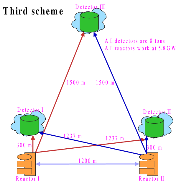
Figure 6: Third scheme: we arrange three detectors symmetrically also, but from the near detectors, the two reactors are not equidistant.

References

- [1] B. Pontecorvo and J. Exptl, Theoret. Phys. 34 (1958) 247; B. Pontecorvo and ZH. Eksp, Teor. Fiz. 53 (1967) 1717;Z. Maki,M. Nakagawa and S. Sakata, Prog. Theor. Phys. 28 (1962) 870.
- [2] Y. Fukuda , Phys. Rev. Lett. 82 (1999) 2644; T. Toshito , hep-ex/0105023; S. Fukuda , Phys. Rev. Lett 86 (2001) 5651.
- [3] M. H. Ahn , Phys. Rev. Lett. 90 (2003) 041801.
- [4] S.P. Mikheyev, A.Yu. Smirnov, Sov. J. Nucl. Phys. 6, 913 (1985); L. Wolfenstein, Phys. Rev. D17, 2369 (1978); S.P. Mikheyev and A.Yu. Smirnov, Yad. Fiz., 42, 1441 (1985); Nuovo Cim 9C, 17 (1986).
- [5] VLBL Study Group H2B-1 (He-sheng Chen et al.). IHEP-EP-2001-01, 2001, hep-ph/0104266.
- [6] M. Aoki, K. Hagiwara, Y. Hayato, T. Kobayashi, T. Nakaya, K. Nishikawa and N. Okamura, Phys.Rev. D67 (2003) 093004; J. Burguet-Castell, D. Casper, J. J. Gomez-Cadenas, P.Hernandez and F.Sanchez, hep-ph/0312068; M. Aoki, K. Hagiwara and N. Okamura, hep-ph/0311324.
- [7] M. Apollonio , Phys. Lett. B420 (1998) 397; M. Apollonio , Phys. Lett. B466 (1999) 415; M. Apollonio , Eur. Phys. J. C27 (2003) 331-374.
- [8] M. Narayan, G. Rajasekaran and S. Uma Sankar, Phys.Rev. D58 (1998) 031301.
- [9] S. M. Bilenky, D. Nicolo and S. T. Petcov, Phys.Lett. B538 (2002) 77.
- [10] G.L. Fogli, E. Lisi, A. Marrone, D. Montanino and A. Palazzo, talk given at 36th Rencontres de Moriond: Electroweak Interactions and Unified Theories, Les Arcs, France, 10-17 Mar 2001, hep-ph/0104221.
- [11] L. A. Mikaelyan and V. V. Sinev, Phys. Atom. Nul. 63 (2000) 1002; V. Mantemyanov, L. Mikaelyan, V. Sinev, V. Kopeikin and Y. Kozlov, Phys. Atom. Nucl. 66 (2003) 1934.
- [12] Y. F. Wang, B. L. Young, et al, talk given at conference “STUDYING NEUTRINO OSCILLATION BY USING DAYA BAY NUCLEAR POWER PLANT AS THE NEUTRINO SOURCE”, Hong Kong, November 28-29, 2003.
- [13] W. Buchmuller, D. Wyler, Phys. Lett. B521 (2001) 291.
- [14] H. Minakata, H. Sugiyama, O. Yasuda, K. Inous and F. Suekane, Phys. Rev. D 68 (2003) 033017.
- [15] P. Huber, M. Lindner, T. Schwetz and W. Winter, Nucl. Phys. B 665 (2003) 487; P. Huber, M. Lindner, M. Rolinec, T. Schwetz and W. Winter, hep-ph/0403068
- [16] P. Vogel and J. Engel, Phys. Rev. D 39 (1989) 3378; H. Murayama and A. Pierce, Phys.Rev. D65 (2002) 013012.
- [17] K. Eguchi , Phys. Rev. Lett. 90 (2003) 021802.
- [18] C. Bemporad, Proceedings of the 3rd International Work-shop on Neutrino Telescopes, Venice (1991).
- [19] G. J. Feldman and R. D. Cousins, Phys. Rev. D 57 (1998) 3873
- [20] Y. F. Wang, talks given in “Workshop on the feasibility study of the DaYa Bay reactor neutrino experiment”, Beijing, Jan. 2004.