Renormalized thermodynamics from the 2PI effective action

High-temperature resummed perturbation theory is plagued by poor convergence properties. The problem appears for theories with bosonic field content such as QCD, QED or scalar theories. We calculate the pressure as well as other thermodynamic quantities at high temperature for a scalar one-component field theory, solving a three-loop 2PI effective action numerically without further approximations. We present a detailed comparison with the two-loop approximation. One observes a strongly improved convergence behavior as compared to perturbative approaches. The renormalization employed in this work extends previous prescriptions, and is sufficient to determine all counterterms required for the theory in the symmetric as well as the spontaneously broken phase.

1 Introduction and overview

All information about the quantum theory can be obtained from the effective action, which is the generating functional for Green’s functions. Typically, the (1PI) effective action $\Gamma[\phi]$ is represented as a functional of the field expectation value or one-point function $\phi$ only. In contrast, the so-called two-particle irreducible (2PI) effective action $\Gamma[\phi,D]$ is written as a functional of $\phi$ and the connected two-point function $D$ [1]. The latter provides an efficient description of quantum corrections in terms of resummed loop-diagrams. The different functional representations of the effective action are equivalent in the sense that they are generating functionals for Green’s functions including all quantum/statistical fluctuations and agree by construction in the absence of sources. However, e.g. loop expansions of the 1PI effective action to a given order in the presence of the “background” field $\phi$ differ in general from a loop expansion of $\Gamma[\phi,D]$ in the presence of $\phi$ and $D$.

This observation has been successfully used in nonequilibrium quantum field theory to resolve the problems of secularity and late-time universality [2, 3] of perturbative approximations, which render the latter invalid even for arbitrarily small couplings [4]. Both the far-from-equilibrium behavior as well as the late-time thermal equilibrium results can be described from a loop expansion of the 2PI effective action without further assumptions for scalar [2, 5] and fermionic theories [6]. Similar results have been obtained using a two-particle irreducible $1/N$ expansion beyond leading order [3, 7, 8].

The same techniques can be applied directly in thermal equilibrium, where efficient formulations in Euclidean space-time become available. In contrast to the far-from-equilibrium case, there are various powerful approximation schemes known in thermal field theory. A prominent approach in equilibrium high-temperature field theory is the so-called “hard-thermal-loop” resummation [9]. However, explicit calculations of thermodynamic quantities such as pressure or entropy typically reveal a poor convergence except for extremely small couplings. An important example for this behavior concerns high-temperature gauge theories. Recent strong efforts to improve the convergence aim at connecting to available lattice QCD results, for which high temperatures are difficult to achieve. In order to find improved approximation schemes it is important to note that the problem is not specific to gauge field theories. Indeed it has been documented in the literature in great detail that problems of convergence of perturbative approaches at high temperature can already be studied in simple scalar theories. For recent reviews in this context see Ref. [10].

A promising candidate for an improved convergence behavior is the loop or coupling expansion of the 2PI effective action. So far, thermodynamic quantities such as pressure or entropy have been mainly calculated to two-loop order. However, aspects of convergence can be sensefully discussed only beyond two-loop order since the one-loop high-temperature result corresponds to the free gas approximation. Efforts to calculate pressure beyond two loops include so-called approximately self-consistent approximations [11], as well as estimates based on further perturbative expansions in the coupling and a variational mass parameter [13]. These studies indicate already improved convergence properties. However, perturbatively motivated estimates as in Ref. [13] suffer from the presence of nonrenormalizable, ultraviolet divergent contributions and the apparent breakdown of the approach beyond some value for the coupling. If one does not want to rely on these further assumptions, going beyond two-loop order requires the use of efficient numerical techniques. Such rigorous studies are important to get a decisive answer about the properties of 2PI expansions. As it turns out (cf. below) these problems appear as an artefact of the additional approximations employed and cannot be attributed to the 2PI loop expansion.

Figure 1: Pressure as a function of the renormalized coupling, normalized to the ideal gas, i.e. one-loop pressure. Shown are the 2PI two- and three-loop results (left) for $T=2T_{0}$ with $T_{0}=m_{R}(T_{0})$. The right figure shows the perturbative results to order $g_{R}^{2}$ and $g_{R}^{3}$ along with the 2PI two-loop curve in the high-temperature limit for illustration of the problematic alternating behavior of perturbation theory (see text).

In this work we calculate the pressure as well as other thermal quantities for a scalar $g^{2}\phi^{4}$ field theory from a three-loop 2PI effective action numerically without further approximations. A detailed comparison with the two-loop approximation is presented. We observe a strongly improved convergence behavior as compared to perturbative approaches. This is exemplified in Fig. 1, where the pressure is shown as a function of the renormalized coupling $g_{R}$ determined by the physical four-vertex. The left figure compares the two- and three-loop result normalized to the ideal gas pressure. For the employed high temperature $T=2m_{R}(T_{0})$ the three-loop corrections to the pressure are rather small. Here $m_{R}(T_{0})$ is the temperature-dependent renormalized mass parameter or inverse correlation length and we have $T_{0}=m_{R}(T_{0})$. For illustration we also show on the right of Fig. 1 the perturbative results to order $g_{R}^{2}$ and $g_{R}^{3}$ along with the dominant 2PI two-loop result for the high-temperature limit. The problematic alternating behavior of the perturbative series is not specific to the limit $T\gg T_{0}$ and is characteristic for higher orders as well [15]. (Cf. Secs. 2.2 and 3.2.)

We obtain the renormalized correlation functions or proper vertices as functions of temperature, building on a renormalization put forward in Refs. [16, 17] (cf. also [18]). In contrast to previous approaches, the renormalization employed in this work is formulated for the resummed 1PI effective action which is calculated from a given loop approximation of the 2PI effective action. The procedure is sufficient to determine all counterterms required for the theory in the symmetric as well as spontaneously broken phase. This extends previous prescriptions, which are not sufficiently general to renormalize the theory in the presence of a non-vanishing field. In particular, they do not renormalize all functional field-derivatives of the effective action even in the symmetric phase. The latter represent the proper vertices, which encode important information about the theory. This is discussed in Sec. 2.1 taking into account three-loop corrections. The considered approximation represents a simple explicit example of a systematic renormalization scheme for 2PI effective actions, which will be given for general approximations in a separate publication [21].

To put our calculations in a more general context, we note that our results for the two- and three-loop approximations of the 2PI effective action are identical to the corresponding two- and three-loop approximations for $n$-particle irreducible ($n$PI) effective actions with arbitrary $n\geq 3$. The agreement up to the considered order is a consequence of an equivalence hierarchy for $n$PI effective actions [22]. Their functional dependence takes into account the propagator as well as the proper three-vertex, four-vertex, …, $n$-vertex [1, 23, 24, 22]. Therefore, a loop expansion of the $n$PI effective action with $n>2$ treats propagators and the respective vertices on the same footing, while a 2PI loop expansion singles out propagator resummation a priori. However, the difference to the 2PI results in the symmetric phase appears only at four-loop order [22], which is beyond the approximation employed in this work. As a consequence, the good convergence properties of the expansion, which we observe, may be attributed to the $n$PI loop expansion with arbitrary $n>2$ rather than to the 2PI loop expansion.

2 Renormalized thermodynamics

We consider a quantum field theory with classical action

$$S=\int{\rm d}^{4}x\left\{\frac{1}{2}\left(\partial_{\mu}\phi\partial^{\mu}\phi-m^{2}\phi^{2}\right)-g^{2}\phi^{4}\right\}\,,$$ (2.1)

where $\phi(x)$ is a real scalar field with bare mass term $m^{2}$ and coupling $g^{2}$. The normalization of the coupling is chosen for simple comparison with existing literature (cf. e.g. Ref. [11]) in view of applications of these methods to QCD thermodynamics. We use the shorthand notation $\int_{x}\equiv\int_{0}^{-i/T}{\rm d}x^{0}\int{\rm d}^{3}x$ with temperature $T$. Following [1] it is convenient to parametrize the temperature dependent 2PI effective action as

$$\Gamma[\phi,D]=S[\phi]+\frac{i}{2}\hbox{Tr}\ln D^{-1}+\frac{i}{2}\hbox{Tr}D_{0}^{-1}(\phi)D+\Gamma_{2}[\phi,D]+{\rm const}\,,$$ (2.2)

which expresses $\Gamma$ in terms of the classical action $S$ and correction terms including the function $\Gamma_{2}$ to which only two-particle irreducible diagrams contribute. Here the classical inverse propagator is given by $iD_{0}^{-1}(x,y;\phi)\equiv\delta^{2}S[\phi]/\delta\phi(x)\delta\phi(y)$. In the absence of external sources physical solutions require

$$\frac{\delta\Gamma[\phi,D]}{\delta\phi(x)}\Big{|}_{\phi=\phi_{0}} = 0\,,$$ (2.3)

$$\frac{\delta\Gamma[\phi,D]}{\delta D(x,y)}\Big{|}_{D=D(\phi)} = 0\,.$$ (2.4)

The 2PI effective action evaluated at $D(\phi;x,y)$, i.e. for the $\phi$-dependent solution of (2.4), is identical to the 1PI effective action $\Gamma[\phi,D(\phi)]$. The effective action at the stationary point, $\Gamma[\phi_{0},D(\phi_{0})]$, corresponds to the logarithm of the partition function in the absence of sources [1]. Therefore, in thermal equilibrium with temperature $T$ ($\phi_{0}$ constant) the effective action is related to the pressure $P$ by

$$P=\frac{T}{L_{3}}i\Gamma[\phi_{0},D(\phi_{0})]\,,$$ (2.5)

where $L_{3}=\int{\rm d}^{3}x$ denotes the spatial volume and the constant in Eq. (2.2) is chosen such that the pressure vanishes at zero temperature. Entropy density ${\mathcal{S}}$ and energy density ${\mathcal{E}}$ are given by

$${\mathcal{S}} = \frac{\partial P}{\partial T}\,,$$ (2.6)

$${\mathcal{E}} = -P+T{\mathcal{S}}=T^{2}\frac{\partial}{\partial T}\left(\frac{P}{T}\right)\,.$$ (2.7)

We recall that all the physical information is contained in the effective action at the stationary point $\Gamma[\phi_{0},D(\phi_{0})]$ and its changes with respect to variations in the field $\phi$ evaluated at $\phi=\phi_{0}$. For instance, the connected two-point function, $\Gamma^{(2)}$, and proper four-point function, $\Gamma^{(4)}$, are given by

$$\Gamma^{(2)}(x,y) \equiv \frac{\delta^{2}\Gamma[\phi,D(\phi)]}{\delta\phi(x)\delta\phi(y)}\Big{|}_{\phi=\phi_{0}}\,,$$ (2.8)

$$\Gamma^{(4)}(x,y,z,w) \equiv \frac{\delta^{4}\Gamma[\phi,D(\phi)]}{\delta\phi(x)\delta\phi(y)\delta\phi(z)\delta\phi(w)}\Big{|}_{\phi=\phi_{0}}\,.$$ (2.9)

All information about the quantum theory can therefore be conveniently obtained from $\Gamma[\phi,D(\phi)]$ by functional differentiation. In particular, $\Gamma[\phi,D(\phi)]$ evaluated for constant field $\phi$ encodes the effective potential.

2.1 Renormalization

The effective action $\Gamma[\phi,D(\phi)]$ is defined in a standard way by suitable regularization, as e.g. lattice regularization or dimensional regularization, and renormalization conditions. We employ renormalization conditions for the two-point function (2.8) and four-point function (2.9), which in Fourier space read:

$$Z\,\Gamma^{(2)}(p^{2})|_{p=0} = -m_{R}^{2}\,,$$ (2.10)

$$Z\,\frac{d}{dp^{2}}\Gamma^{(2)}(p^{2})|_{p=0} = -1\,,$$ (2.11)

$$Z^{2}\,\Gamma^{(4)}(p_{1},p_{2},p_{3})|_{p_{1}=p_{2}=p_{3}=0} = -4!\,g^{2}_{R}\,,$$ (2.12)

with the wave function renormalization $Z$. Here the renormalized mass parameter $m_{R}$ corresponds to the inverse correlation length. The physical four-vertex at zero momentum is given by $g^{2}_{R}$. Without loss of generality we use throughout this work renormalization conditions for $\phi_{0}=0$.

We emphasize that at non-zero temperature the mass parameter as well as the four-vertex are temperature dependent. The value of the mass and coupling at a given temperature and momentum scale uniquely determines the theory. This can then be used to calculate properties at some other temperature. We will typically define the theory by giving renormalization conditions at zero temperature as well as some non-zero temperature $T_{0}$ with $m_{R}\equiv m_{R}(T_{0})$ and $g_{R}\equiv g_{R}(T_{0})$.

2.1.1 2PI renormalization scheme to order $g_{R}^{4}$

In order to impose the renormalization conditions (2.10)–(2.12) one first has to calculate the solution for the two-point field $D(\phi)$ for $\phi=0$, which encodes the resummation and which is obtained from the stationarity condition for the 2PI effective action (2.4). To achieve this we will for the most part follow the lines of the renormalization procedure described in Ref. [17]. We comment on the additional implications, which arise from imposing (2.10)–(2.12), below. For further details we refer to Ref. [21]. Here we will explicitly demonstrate from the numerical solution of the three-loop approximation that the renormalized quantities are insensitive to the change of the (lattice) regularization.

The renormalized field is $\phi_{R}=Z^{-1/2}\phi$. It is convenient to introduce the counterterms relating the bare and renormalized variables in a standard way with

$$Zm^{2}=m_{R}^{2}+\delta m^{2}\,\,,\qquad Z^{2}g^{2}=g^{2}_{R}+\delta g^{2}\,\,,\qquad\delta Z=Z-1\,,$$ (2.13)

and we write

$$D(\phi)=ZD_{R}(\phi_{R})\,\,.$$ (2.14)

In terms of the renormalized quantities the classical action (2.1) reads

$$S = \int_{x}\Bigg{(}\frac{1}{2}\partial_{\mu}\phi_{R}\partial^{\mu}\phi_{R}-\frac{1}{2}m_{R}^{2}\phi_{R}^{2}-g^{2}_{R}\phi_{R}^{4}$$ (2.15)

$$+\frac{1}{2}\delta Z\partial_{\mu}\phi_{R}\partial^{\mu}\phi_{R}-\frac{1}{2}\delta m^{2}\phi_{R}^{2}-\delta g^{2}\phi_{R}^{4}\Bigg{)}\,.$$

Similarly, one can write for the one-loop part $\hbox{Tr}\ln D^{-1}=\hbox{Tr}\ln D_{R}^{-1}$ up to an irrelevant, temperature independent constant. The next term of Eq. (2.2) can be written as

$$\frac{i}{2}\hbox{Tr}\,D_{0}^{-1}(\phi)D(\phi) = -\frac{1}{2}\int_{x}\left(\square_{x}+m_{R}^{2}+\delta Z_{1}\,\square_{x}+\delta m_{1}^{2}\right)D_{R}(x,y;\phi_{R})|_{x=y}$$ (2.16)

$$-6\left(g^{2}_{R}+\delta g_{1}^{2}\right)\int_{x}\phi_{R}^{2}(x)D_{R}(x,x;\phi_{R})\,.$$

Here $\delta Z_{1}$, $\delta m_{1}^{2}$ and $\delta g_{1}^{2}$ denote the same counterterms as introduced in (2.13), however, approximated to the given order. To express $\Gamma_{2}$ in terms of renormalized quantities it is useful to note the identity

$$\Gamma_{2}[\phi,D(\phi)]|_{g^{2}}=\Gamma_{2}[\phi_{R},D_{R}(\phi_{R})]|_{g^{2}_{R}+\delta g^{2}}\,,$$ (2.17)

which simply follows from the standard relation between the number of vertices, lines and fields by counting factors of $Z$. Therefore, one can replace in $\Gamma_{2}$ the bare field and propagator by the renormalized ones if one replaces bare by renormalized vertices as well. We emphasize that mass and wavefunction renormalization counterterms, $\delta Z$ and $\delta m^{2}$, do not appear explicitly in $\Gamma_{2}$. This can be understood from the fact that the only two-particle irreducible diagrams with mass and field strength insertions are those displayed in Fig. 2. The counterterms in the classical action (2.15), in the one-loop term (2.16) and beyond one-loop contained in $\Gamma_{2}$ have to be calculated for a given approximation of $\Gamma_{2}$. Here we consider the 2PI effective action to order $g_{R}^{4}$ with

$$\Gamma_{2}[\phi_{R},D_{R}(\phi_{R})] \!\!=\!\! -3g_{R}^{2}\int_{x}D_{R}^{2}(x,x;\phi_{R})+i48g_{R}^{4}\int_{xy}\phi_{R}(x)D_{R}^{3}(x,y;\phi_{R})\phi_{R}(y)$$ (2.18)

$$+i12g_{R}^{4}\int_{xy}D_{R}^{4}(x,y;\phi_{R})-3\delta g_{2}^{2}\int_{x}D_{R}^{2}(x,x;\phi_{R})\,,$$

where the last term contains the respective coupling counterterm at two-loop. There are no three-loop counterterms since the divergences arising from the three-loop contribution in (2.18) are taken into account by the lower counterterms [17, 21]. The coupling counterterms are displayed diagrammatically in Fig. 3.

Figure 2: Diagrammatic representation of the mass and field strength counterterms. The cross in the left graph denotes indistinctly the mass counterterm $\delta m_{1}^{2}$ or field strength counterterm $\delta Z_{1}^{2}$ appearing in Eq. (2.16), while the one in the right graph represents the $\delta m^{2}$ and $\delta Z^{2}$ insertions in Eq. (2.15). The line of the closed loop represents $D_{R}$, while a circled cross denotes $\phi_{R}$.

One first has to calculate the solution $D_{R}(\phi_{R})$ obtained from the stationarity condition (2.4) for the 2PI effective action. For this one has to impose the same renormalization condition as for the propagator (2.10) in Fourier space:

$$iD_{R}^{-1}(p^{2};\phi_{R})|_{p=0,\phi_{R}=0}=-m_{R}^{2}\,,$$ (2.19)

for given finite renormalized “four-point” field

$$V_{R}(x,y;z,w)\equiv\frac{\delta^{2}iD_{R}^{-1}(x,y;\phi_{R})}{\delta\phi_{R}(z)\phi_{R}(w)}\Big{|}_{\phi_{R}=0}\,.$$ (2.20)

Figure 3: Diagrammatic representation of the coupling counterterms. Here the vertices denote $\delta g_{2}^{2}$, $\delta g_{1}^{2}$ and $\delta g^{2}$, respectively, which appear in Eqs. (2.18), (2.16) and (2.15).

For the above approximation we note the identity

$$\frac{\delta^{2}\Gamma[\phi_{R},D_{R}(\phi_{R})]}{\delta\phi_{R}(x)\phi_{R}(y)}\Big{|}_{\phi_{R}=0}\equiv iD_{R}^{-1}(x,y;\phi_{R})|_{\phi_{R}=0}$$ (2.21)

for

$$\delta Z=\delta Z_{1}\quad,\quad\delta m^{2}=\delta m_{1}^{2}\quad,\quad\delta g_{1}^{2}=\delta g_{2}^{2}\,,$$ (2.22)

such that (2.19) for $D_{R}$ is trivially fulfilled. In contrast to the exact theory, for the 2PI effective action to order $g_{R}^{4}$ a similar identity does not connect the proper four-vertex with $V_{R}$. Here the respective condition for the four-point field $V_{R}$ in Fourier space reads

$$V_{R}(p_{1},p_{2},p_{3})|_{p_{1}=p_{2}=p_{3}=0}=-4!\,g^{2}_{R}\,.$$ (2.23)

Note that this has to be the same as for the four-vertex (2.12). For the universality class of the $\phi^{4}$ theory there are only two independent input parameters, which we take to be $m_{R}$ and $g^{2}_{R}$, and for the exact theory $V_{R}$ and the four-vertex agree. The renormalization conditions (2.10)–(2.12) for the propagator and four-vertex, together with the 2PI scheme (2.19)–(2.23) provides an efficient fixing of all the above counterterms. In particular, it can be very conveniently implemented numerically, which turns out to be crucial for calculations beyond order $g_{R}^{2}$.

The apparent insensitivity of the renormalized quantities with respect to changes in the (lattice) regularization is demonstrated for the temperature dependent four-point field $V_{R}(T)$ in Fig. 4. The upper solid and dashed line show the results for $V_{R}(T)$ as a function of the logarithm of the lattice cutoff for two temperatures $T=2T_{0}$ and $T=3T_{0}$. Here $T_{0}$ is fixed by $T_{0}=m_{R}(T_{0})$ and the lattice volume is kept constant with $Lm_{R}(T_{0})=2$. For illustration we also show the behavior of $V_{R}(T)$ if the renormalization is not done properly. This is achieved by replacing in the three-loop contribution of (2.18) $g_{R}^{4}$ by the “bare” coupling $(g_{R}^{2}+\delta g_{3}^{2})^{2}$ and taking $\delta g_{3}^{2}=\delta g_{1}^{2}$. The induced strong logarithmic cutoff dependence of $V_{R}(T)$ can be observed from the respective results displayed in the lower curves of Fig. 4.

Figure 4: The upper solid and dashed line show the results for $V_{R}(T)$ as a function of the logarithm of the lattice cutoff for two temperatures $T=2T_{0}$ and $T=3T_{0}$. Here $T_{0}$ is fixed by $T_{0}=m_{R}(T_{0})$ and $V_{R}(T_{0})=-1$. For illustration we also show results for the same quantity (lower curves) if the renormalization is not done properly, by adding a “naive” three-loop coupling counterterm as explained in the text. (The “oscillation” is a lattice artefact arising from Fourier transformation of odd or even arrays.)

We emphasize that the current approximation (2.18) for the 2PI effective action can only be expected to be valid for sufficiently small $\phi_{R}\ll m_{R}/g_{R}$. If the latter is not fulfilled there are additional ${\mathcal{O}}(g_{R}^{4})$ contributions at three-loop $\sim g_{R}^{6}\phi_{R}^{2}$ and $\sim g_{R}^{8}\phi_{R}^{4}$. The approximation should therefore not be used to study the theory in the spontaneously broken phase or near the critical temperature of the second-order phase transition. For studies of the latter using the 2PI effective action see Ref. [25]. Here we will investigate how the 2PI effective action cures convergence problems of high-temperature perturbation theory, for which the approximation (2.18) provides the correct generating functional up to order $g_{R}^{6}$ corrections, including all three-loop corrections in the high-temperature phase.

2.1.2 Renormalized equations for the two- and four-point functions

¿From the 2PI effective action to order $g_{R}^{4}$ we find with $\delta g_{1}^{2}=\delta g_{2}^{2}$ from (2.22) for the two-point function:

$$iD_{R}^{-1}(x,y;\phi_{R}) \!\!=\!\! -\left[(1+\delta Z_{1})\square_{x}+m_{R}^{2}+\delta m_{1}^{2}\right.$$

$$\left.+12(g_{R}^{2}+\delta g_{1}^{2})\left(D_{R}(x,x;\phi_{R})+\phi_{R}^{2}(x)\right)\right]\delta(x-y)$$

$$+i288g_{R}^{4}D_{R}^{2}(x,y;\phi_{R})\phi_{R}(x)\phi_{R}(y)+i96g_{R}^{4}D_{R}^{3}(x,y;\phi_{R})\,.$$

According to (2.21) this expression coincides with the one for the propagator $\delta^{2}\Gamma[\phi_{R},D_{R}(\phi_{R})]/\delta\phi_{R}(x)\delta\phi_{R}(y)$ at $\phi_{R}=0$. It is straightforward to verify this using

$$\frac{\delta\Gamma[\phi_{R},D_{R}(\phi_{R})]}{\delta\phi_{R}(x)}\equiv\frac{\delta\Gamma[\phi_{R},D_{R}]}{\delta\phi_{R}(x)}\,,$$ (2.25)

which is valid since the variation of $D_{R}(\phi_{R})$ with $\phi_{R}$ does not contribute due to the stationarity condition (2.4). The four-point field (2.20) in this approximation is given by

$$V_{R}(x,y;z,w) = -24(g_{R}^{2}+\delta g_{1}^{2})\delta(x-y)\delta(x-z)\delta(x-w)$$ (2.26)

$$-12(g_{R}^{2}+\delta g_{1}^{2})\frac{\delta^{2}D_{R}(x,x;\phi_{R})}{\delta\phi_{R}(z)\delta\phi_{R}(w)}\Big{|}_{\phi_{R}=0}\delta(x-y)$$

$$+i\frac{(24g_{R}^{2})^{2}}{2}\Bigg{(}\delta(x-w)\delta(y-z)+\delta(y-w)\delta(x-z)$$

$$+\frac{\delta^{2}D_{R}(x,y;\phi_{R})}{\delta\phi_{R}(z)\delta\phi_{R}(w)}\Big{|}_{\phi_{R}=0}\Bigg{)}D_{R}^{2}(x,y;\phi_{R}=0)\,.$$

Inserting the chain rule formula

$$\frac{\delta^{2}iD_{R}(x,y;\phi_{R})}{\delta\phi_{R}(z)\delta\phi_{R}(w)}\Big{|}_{\phi_{R}=0}=-\left.\int_{u,v}D_{R}(x,u;\phi_{R})V_{R}(u,v;z,w)D_{R}(v,y;\phi_{R})\right|_{\phi_{R}=0}\,$$ (2.27)

into Eq. (2.26) one arrives at the Bethe-Salpeter type equation for $V_{R}$ discussed in Refs. [16, 17]. Eqs. (2.26) and (LABEL:eq:invD) form a closed set of equations for the determination of the counterterms $\delta Z_{1}$, $\delta m_{1}^{2}$ and $\delta g_{1}^{2}$. Together with $(\ref{eq:renconst})$ one observes that $\delta g^{2}$ would be undetermined from these equations alone as employed in Refs. [16, 17]. This counterterm is determined by taking into account the equation for the physical four-vertex, which is obtained from the above 2PI effective action as

$$\frac{\delta^{4}\Gamma[\phi_{R},D_{R}(\phi_{R})]}{\delta\phi_{R}(x)\delta\phi_{R}(y)\delta\phi_{R}(z)\delta\phi_{R}(w)}\Big{|}_{\phi_{R}=0}=-24(g_{R}^{2}+\delta g^{2})\delta(x-y)\delta(x-z)\delta(x-w)$$

$$+V_{R}(x,y;z,w)+V_{R}(x,z;y,w)+V_{R}(x,w;y,z)$$

$$-2\left.\left(\frac{\delta iD_{R}^{-1}(x,y;\phi_{R})}{\delta D_{R}(z,w)}+\frac{\delta iD_{R}^{-1}(x,z;\phi_{R})}{\delta D_{R}(y,w)}+\frac{\delta iD_{R}^{-1}(x,w;\phi_{R})}{\delta D_{R}(y,z)}\right)\right|_{\phi_{R}=0}\,,$$

(2.28)

where from (LABEL:eq:invD) one uses the relation

$$\left.\frac{\delta iD_{R}^{-1}(x,y;\phi_{R})}{\delta D_{R}(z,w)}\right|_{\phi_{R}=0} = -12(g_{R}^{2}+\delta g_{2}^{2})\delta(x-y)\delta(x-z)\delta(x-w)$$ (2.29)

$$+i\frac{(24g_{R}^{2})^{2}}{2}D_{R}^{2}(x,y;\phi_{R}=0)\delta(x-z)\delta(y-w)\,.$$

We emphasize that the counterterm $\delta g^{2}$ plays a crucial role in the broken phase, since it is always multiplied by the field $\phi_{0}$ and hence it is essential for the determination of the effective potential. It is also required in the symmetric phase, in particular, when one calculates the thermal coupling using Eq. (2.28).

2.2 Analytical example: 2PI two-loop order

It is instructive to consider first the 2PI effective action to two-loop order for which much can be discussed analytically. In this case $Z=1$ for the scalar theory and the renormalized vacuum mass $m_{R}=m_{R}(T=0)$ of Eq. (2.10) or, equivalently, of Eq. (2.19) is given to this order by

$$\frac{m_{R}^{2}}{g^{2}} = 12\,\mu^{\epsilon}\!\int\frac{{\rm d}^{d}k}{(2\pi)^{d}}\left(k^{2}+m_{R}^{2}\right)^{-1}+\frac{m^{2}}{g^{2}}$$ (2.30)

$$= -\frac{3m_{R}^{2}}{2\pi^{2}}\left(\frac{1}{\epsilon}-\ln\frac{m_{R}}{\bar{\mu}}+\frac{1}{2}\right)+\frac{m^{2}}{g^{2}}\,,$$

where $m^{2}=m_{R}^{2}+\delta m_{1}^{2}$ and $g^{2}=g_{R}^{2}+\delta g_{1}^{2}$ is the zero temperature coupling $g_{R}=g_{R}(T=0)$ and we have used (2.22). Here we have employed dimensional regularization and evaluated the integral in $d=4-\epsilon$ for Euclidean momenta $k$. The bare coupling in the action (2.1) has been rescaled accordingly, $g^{2}\to\mu^{\epsilon}g^{2}$, and is dimensionless; $\bar{\mu}^{2}\equiv 4\pi e^{-\gamma_{E}}\mu^{2}$ and $\gamma_{E}$ denotes Euler’s constant. Below we will employ a lattice regularization for comparison and to go beyond two-loop order.

Similarly, the zero-temperature four-point function resulting from Eq. (2.23) for the 2PI effective action to order $g_{R}^{2}$ is given by

$$g^{2}_{R} = g^{2}-12g^{2}g^{2}_{R}\,\mu^{\epsilon}\!\int\frac{{\rm d}^{d}k}{(2\pi)^{d}}\left(k^{2}+m_{R}^{2}\right)^{-2}$$ (2.31)

$$= g^{2}-\frac{3g^{2}}{2\pi^{2}}g^{2}_{R}\left(\frac{1}{\epsilon}-\ln\frac{m_{R}}{\bar{\mu}}\right)\,$$

with (2.22). We emphasize that the same equation is obtained starting from the renormalization condition for the proper four-vertex (2.12) with $\delta g^{2}=3\delta g_{1}^{2}$. One observes that all counterterms are uniquely fixed by the renormalization procedure put forward in the previous sections.

At non-zero temperature one obtains renormalized equations for the thermal mass and coupling in terms of the vacuum parameters:

$$m_{R}^{2}(T) = m_{R}^{2}-24g_{R}^{2}P_{0}^{\prime}\left(T,m_{R}^{2}(T)\right)$$ (2.32)

$$+\frac{3g^{2}_{R}}{4\pi^{2}}\left(m_{R}^{2}(T)\log\frac{m^{2}_{R}(T)}{m^{2}_{R}}-m_{R}^{2}(T)+m_{R}^{2}\right)\,,$$

$$\frac{1}{V_{R}(T)} = -\frac{1}{4!g^{2}_{R}}-P_{0}^{\prime\prime}(T,m_{R}^{2}(T))\,,$$ (2.33)

$$g^{2}_{R}(T) = \frac{3}{1/g^{2}_{R}+4!P_{0}^{\prime\prime}(T,m_{R}^{2}(T))}-2g_{R}^{2}\,,$$ (2.34)

where $P_{0}$ denotes the pressure of the free gas:

$$P_{0}(T,m^{2}_{R}(T))=-T\int\frac{{\rm d}^{3}p}{(2\pi)^{3}}\ln\left(1-e^{-\omega_{\bf p}(T)/T}\right)\,.$$ (2.35)

with $\omega_{\bf p}(T)=\sqrt{{\bf p}^{2}+m^{2}_{R}(T)}$ and $P_{0}^{\prime}(T,m_{R}^{2}(T))$ and $P_{0}^{\prime\prime}(T,m_{R}^{2}(T))$ denote its first and second derivative with respect to $m_{R}^{2}(T)$.

The pressure to two-loop order is given by

$$P_{2}=P_{0}(T,m^{2}_{R}(T))-\frac{1}{2}m_{R}^{2}(T)P_{0}^{\prime}(T,m_{R}^{2}(T))+\frac{m_{R}^{4}(T)-m_{R}^{4}}{128\pi^{2}}$$

$$-\frac{1}{16}\left(\frac{1}{3g^{2}_{R}}+\frac{1}{4\pi^{2}}\right)\left(m_{R}^{2}(T)-m_{R}^{2}\right)m_{R}^{2}\,.$$ (2.36)

We have used these analytical formulae to check the (two-loop) numerics for the continuum and thermodynamic limit. We have also checked, that for the employed parameters the zero temperature limit is already reached for $T\leq m_{R}(T_{0})/8$. We use this below to numerically estimate the observables in vacuum.

The scalar $\phi^{4}$-theory in $3+1$ dimensions is non-interacting if it is considered as a fundamental theory valid for arbitrarily high momentum scales. This is the so-called “triviality” of $\phi^{4}$-theory [27]. However, if the theory is considered as a low-momentum effective theory with a physical highest momentum then the renormalized coupling $g_{R}$ can be non-zero. A non-vanishing zero-momentum four-vertex $g_{R}$ requires both a highest momentum cutoff and an “infrared cutoff” such as a non-zero mass term $m_{R}$. This can be conveniently discussed by introducing a scale $\Lambda$ with

$$\frac{3}{2\pi^{2}}\ln\frac{\Lambda}{\bar{\mu}}\equiv\frac{1}{g^{2}}+\frac{3}{2\pi^{2}\epsilon}\,.$$ (2.37)

In terms of this scale the renormalized coupling (four-vertex) reads

$$g^{2}_{R}=\frac{2\pi^{2}}{3\ln\frac{\Lambda}{m_{R}}}\,.$$ (2.38)

As a consequence, the zero-temperature coupling $g^{2}_{R}$ vanishes for $m_{R}/\Lambda\to 0$, i.e. by either sending $\Lambda\to\infty$ for fixed $m_{R}$ or by taking $m_{R}\to 0$ for fixed scale $\Lambda$. For given $\Lambda/m_{R}$ the renormalized coupling takes on its finite maximum value (2.38) for a diverging $g$ due to the Landau pole in the equation for the coupling counterterm $\delta g^{2}=g^{2}-g_{R}^{2}$ obtained from (2.31) (cf. also the corresponding Fig. 7 for the 2PI three-loop solution).

The high-temperature result can be obtained with non-zero $m_{R}$ for the limit $T\gg m_{R}$, which is conventionally dubbed the massless limit in the literature. To calculate $m_{R}(T)$ it is then useful to rewrite the equation (2.32) in terms of the renormalized four-point function at non-zero temperature, $g_{R}^{2}(T)$, for which the limit $m_{R}\to 0$ can be taken directly (cf. also the discussions in Ref. [10]). Here the two-loop pressure (2.36) in the limit $m_{R}\to 0$ becomes

$$P_{2}(T)=P_{0}(T)+\frac{1}{2}m_{R}^{2}(T)P_{0}^{\prime}(T,m_{R}^{2}(T))+\frac{m_{R}^{4}(T)}{128\pi^{2}}\,,$$ (2.39)

using

$$\lim_{m_{R}\to 0}\frac{m_{R}^{2}}{g_{R}^{2}}=\lim_{m_{R}\to 0}\frac{3}{2\pi^{2}}m_{R}^{2}\ln\frac{\Lambda}{m_{R}}=0\,.$$ (2.40)

It is instructive to compare at this point to perturbation theory since its characteristic problems are apparent already at low orders. In Sec. 3.2 we will discuss aspects of the higher order behavior. To make link with other schemes we note that the $\overline{\rm MS}$ renormalized “running” $V_{R}(\bar{\mu})$ is given by

$$-\frac{4!}{V_{R}(\bar{\mu})}\equiv\frac{1}{g^{2}_{R}}+\frac{3}{2\pi^{2}}\ln\frac{m_{R}}{\bar{\mu}}=\frac{1}{g^{2}}+\frac{3}{2\pi^{2}\epsilon}\,,$$ (2.41)

which can be written explicitly as

$$-\frac{1}{4!}V_{R}(\bar{\mu})=\frac{g^{2}_{R}}{1+\frac{3g^{2}_{R}}{2\pi^{2}}\ln\frac{m_{R}}{\bar{\mu}}}\,.$$ (2.42)

One observes that $V_{R}(\bar{\mu})$ corresponds to the zero-momentum four-vertex $g_{R}^{2}$ for the choice of $\bar{\mu}=m_{R}$.

In perturbation theory the massless or high-temperature limit has been particularly extensively studied in the literature. Up to order $g_{R}^{4}$ corrections the weak coupling expansion of the pressure for $T\gg m_{R}$ can be obtained starting from (2.36) or (2.39) using the high-temperature expansion of the gap equation (2.32):

$$m_{R}^{2}(T)\simeq g_{R}^{2}T^{2}-\frac{3}{\pi}g_{R}^{2}Tm_{R}(T)\,,$$ (2.43)

where we neglect perturbative terms of order $g_{R}^{4}$ and higher. The first term comes from $12g_{R}^{2}\int\frac{{\rm d}^{3}p}{(2\pi)^{3}}n({\bf p})/|{\bf p}|=g_{R}^{2}T^{2}$ and the second term employs

$$\int\frac{{\rm d}^{3}p}{(2\pi)^{3}}\left(\frac{n(\omega_{\bf p})}{\omega_{\bf p}}-\frac{n({\bf p})}{|{\bf p}|}\right)\,\simeq\,T\int\frac{{\rm d}^{3}p}{(2\pi)^{3}}\left(\frac{1}{{\bf p}^{2}+m_{R}^{2}(T)}-\frac{1}{{\bf p}^{2}}\right)\,=\,-\frac{1}{4\pi}m_{R}(T)T\,,$$

with $n(\omega_{\bf p})=(\exp(\omega_{\bf p}/T)-1)^{-1}$ and where it was used that the momentum integral is dominated by momenta $\sim g_{R}T$ with $n(\omega_{\bf p})\simeq T/\omega_{\bf p}$. Using these approximations in the 2PI two-loop pressure (2.39), the high-temperature perturbative result is obtained as

$$\frac{P_{\rm pert}(T)}{T^{4}}\simeq\frac{\pi^{2}}{90}-\frac{g_{R}^{2}}{48}+\frac{g_{R}^{3}}{12\pi}\,,$$ (2.44)

up to terms of order $g_{R}^{4}$ [10]. The entropy and energy density, respectively, are then given by ${\mathcal{S}}_{\rm pert}(T)\simeq 4P_{\rm pert}(T)/T$ and ${\mathcal{E}}_{\rm pert}(T)\simeq 3P_{\rm pert}(T)$. The perturbative results to order $g_{R}^{2}$ and $g_{R}^{3}$ are displayed in Fig. 1 along with the 2PI two-loop result. The alternating behavior and poor convergence of the perturbative series observed from the low orders in (2.44) manifest itself also at higher orders of $g_{R}$ [15]. This problem of perturbation theory is not specific to the limit $T\gg m_{R}$ but can also be observed for lower $T/m_{R}$. For instance, for $T\ll m_{R}$ the perturbative (positive) order $g_{R}^{4}$ contribution to the pressure is found to dominate the (negative) order $g_{R}^{2}$ contribution for not too small coupling [15].

3 Numerical calculation to three-loop order

In order to obtain the results for the 2PI effective action to three-loop order without further approximations, we use numerical (lattice) techniques. The employed hypercubic lattice discretization provides a regularization scheme. It turns out to be convenient to carry out the calculation using the unrenormalized propagator $D$ and four-point field $V$, where $V=Z^{-2}V_{R}$ defined with Eq. (2.20). On the lattice we consider Euclidean space-time and in Fourier space we denote the Euclidean two-point field by $\bar{D}_{k}$ and four-point field by $\bar{V}_{k}\equiv\bar{V}(k,-k,0,0)$, without loss of generality. Here $\bar{D}_{k=0}^{-1}=Z^{-1}m_{R}^{2}$, $d\bar{D}_{k}^{-1}/dk^{2}|_{k=0}=Z^{-1}$ and $\bar{V}_{k=0}=24Z^{-2}g_{R}^{2}$ are the Euclidean equivalents of the above renormalization conditions. Following the procedure of Sec. 2.1, for the renormalization one needs with (2.22) to know $g^{2}$, $\delta g^{2}$, $m^{2}$ and $Z$ which are functions of the lattice cutoff. The errors arising from subtracting cutoff dependent quantities such as the quadratic mass contribution of the setting sun diagram remain under control, since the numerical value of the unrenormalized quantities as well as the physical values simultaneously fit into a double precision variable for the employed cutoff values.

On the lattice there is only a subgroup of the rotation symmetry generated by the permutations of $p_{x},p_{y},p_{z}$ and the reflections $p_{x}\leftrightarrow-p_{x}$ etc., which entails a reduction of independent lattice sites by a factor of 48. For three space dimensions, using periodic boundary conditions, a lattice of typical linear size $32a$ requires $N_{s}=969$ independent sites. In the fourth dimension we use a different lattice spacing ($a_{t}$) and lattice size (typically $N_{t}=128$) so the rotation symmetry cannot be extended. We implement two routines that make use of the symmetry features in order to have acceptable performance, the addup function and a four dimensional fast Fourier transformation defined as:

$$\texttt{addup}(\bar{H}) = \frac{1}{L_{4}}\sum_{k}\bar{H}_{k}\,,$$ (3.45)

$$\texttt{fft}(\tilde{H})_{k} = a^{3}a_{t}\sum_{x}\tilde{H}_{x}e^{ikx}\,,$$ (3.46)

$$\texttt{invfft}(\bar{H})_{x} = \frac{1}{L_{4}}\sum_{k}\bar{H}_{k}e^{-ikx}\,,$$ (3.47)

where $L_{4}=N^{3}N_{t}a^{3}a_{t}$ and $\bar{H}$ is a given lattice field in Fourier space. Fields with a tilde ($\tilde{H}$) are in coordinate space. Here $\Sigma_{k}$ (and $\Sigma_{x}$) denotes a summation over all lattice four-momenta (or coordinates) respecting the appropriate symmetry weights.

3.1 Two-loop solution

We first consider the two-loop lattice calculation, which can be compared with the analytic discussion of Sec. 2.2. In this case $\bar{D}_{k}^{-1}=k^{2}+m_{R}^{2}$ and the respective coupling and mass equations on the lattice read

$$1/g^{2} = 1/g_{R}^{2}-12\,\texttt{addup}(\bar{D}^{2})\,,$$ (3.48)

$$m^{2} = m_{R}^{2}-12g^{2}\,\texttt{addup}(\bar{D})\,.$$ (3.49)

We solve for $g^{2}$ and $m^{2}$ for given renormalized parameters as a function of the lattice cutoff. With these bare parameters we calculate the pressure, thermal mass and coupling at various temperatures, using the same lattice spacing. The results are given below along with the order $g_{R}^{4}$ results. The variation of the temperature is implemented by changing the lattice size according to $T=1/(N_{t}a_{t})$.

The pressure is calculated by evaluating the 2PI effective action to this order using Eq. (2.5):

$$P_{2}=\texttt{addup}\left[\frac{1}{2}\log\bar{D}+3g^{2}\bar{D}\texttt{addup}\bar{D}\right]\,.$$ (3.50)

This expression suffers from a temperature independent quartic divergence. To subtract this, we always measure pressure differences, by calculating the pressure at zero temperature as well. We carry out the subtraction before calling the spatial part of the overall addup function. The sum over the fourth dimension has to be done beforehand, since the respective lattice sizes are not the same for different temperatures.

3.2 Three-loop solution

We obtain the renormalized physical results in two steps: At zero temperature or a given temperature $T_{0}$ we numerically solve the equation (LABEL:eq:invD) for the two-point field and the equation (2.26) for the four-point field with the conditions (2.19) and (2.23) simultaneously. This way we obtain the counterterms $\delta g_{1}^{2}$, $\delta Z_{1}$ and $\delta m_{1}$, using (2.22). The counterterm for the coupling in the classical action, $\delta g^{2}$, can then be obtained from Eq. (2.28). At a different temperature $T$ we use the counterterms obtained in the first step to evaluate physical quantities. We solve first Eq. (LABEL:eq:invD) and get the thermal propagator, the thermal mass and the pressure. Then by solving the corresponding equation (2.26) we obtain the four-point function $\bar{V}_{k}(T)$. Finally, the thermal coupling is obtained from Eq. (2.28) using the previously obtained value of $\delta g^{2}$.

In the following we describe the numerical implementation of the simultaneous iterative solution of the propagator and coupling equation in more detail. The renormalized mass, $m_{R}$, is extracted from the low-momentum form of the inverse propagator $\bar{D}_{k}^{-1}=Z^{-1}\left(k^{2}+m_{R}^{2}+{\cal O}(k^{4})\right)$. The renormalized coupling, $g_{R}^{2}$ is obtained from the respective vertex equation for $\bar{V}_{k}$ to this order:

$$\frac{\bar{V}_{k}}{24} = g^{2}-\frac{g^{2}}{2L_{4}}\sum_{q}\bar{D}_{q}^{2}\bar{V}_{q}-24Z^{-4}g_{R}^{4}\bar{F}_{k}+\frac{12Z^{-4}g_{R}^{4}}{L_{4}}\sum_{q}\bar{F}_{k+q}\bar{D}_{q}^{2}\bar{V}_{q}\,,$$ (3.51)

with $\bar{F}_{k}\equiv L_{4}^{-1}\Sigma_{q}\bar{D}_{q}\bar{D}_{k-q}$. We note that both the integrand and the kernel $\bar{F}_{k}$ from the sunset diagram can be calculated by convolution, which is simple if the fft and invfft routines are provided. The numerical implementation of the vertex equation can be summarized as follows:

$\tilde{F}_{x}=\left(\texttt{invfft}(\bar{D})\right)^{2}_{x}$
$\bar{F}_{k}=\texttt{fft}(\tilde{F})_{k}$
begin loop (iterations)
         $\tilde{H}_{x}=\texttt{invfft}(\bar{D}^{2}\bar{V})_{x}$
         $I_{k}=\texttt{fft}(\tilde{F}\tilde{H})_{k}$
         $\bar{V}^{\rm new}_{k}/24=g^{2}-g^{2}{\tilde{H}}_{x=0}/2-24g_{R}^{4}Z^{-4}\bar{F}_{k}+12g_{R}^{4}Z^{-4}I_{k}$
end loop

Similarly, the propagator equation can be implemented by convolutions:

begin loop (iterations)
         $\tilde{D}=\texttt{invfft}(\bar{D})$
         $\bar{D}^{-1,{\rm new}}_{k}=\bar{D}_{0,k}^{-1}+12g^{2}\texttt{addup}(\bar{D})-96g_{R}^{4}Z^{-4}\texttt{fft}({\tilde{D}}^{3})_{k}$
end loop

with $\bar{D}_{0,k}^{-1}=k^{2}+m^{2}$. We emphasize that the simple iterations do not converge well. The iterated propagator and four-point function oscillates around a physically senseful value and sometimes this oscillation is damped slower than the round-off errors accumulate. The alternating behavior at each order in the iteration is exemplified for the zero-momentum propagator in Fig. 5.

Figure 5: Shown is the behavior of the naive iterative solution of the equation for the propagator. Here each number corresponds to the value of $\bar{D}_{k=0}^{-1}$ after the respective number of iterations, starting from the classical propagator $\bar{D}_{0,k}$. The temperature is $T=4m_{R}$ in units of the zero-temperature mass $m_{R}$. One observes convergence only after of order 100 iterations. Iterative solution procedures can nevertheless be very efficiently applied with slight modifications (with a convergence factor of 0.5 convergence is achieved after 14 steps, cf. the discussion in the text).

A more efficient iterative solution procedure involves a convergence factor, which avoids/damps the alternating behavior:

$$\bar{D}_{k}^{-1,{\rm update}}=\alpha\bar{D}_{k}^{-1,{\rm new}}+(1-\alpha)\bar{D}_{k}^{-1}\,.$$ (3.52)

For a choice of $\alpha=0.1\dots 0.5$ convergence was typically achieved after $20\dots 50$ iterations by matching the exit criterium. This criterium is based on the sufficient smallness of the absolute change in $\bar{D}$ or $\bar{V}$ at all momenta.

We note that the naive iterative solution of the equation for the propagator (with $\alpha=1$) reflects some aspects of a perturbative calculation. Starting from the classical propagator, each iteration adds a higher order contribution to $\bar{D}$. At low orders the origin of the problematic oscillating behavior of a perturbative series in $g_{R}$ can be nicely observed from Fig. 5. Though higher orders in the iteration do not take into account all respective perturbative contributions, it is interesting that a convergence is obtained only after of order $100$ (!) iterations.

When fixing the renormalized theory we implement an outer loop for repeating the subsequent solutions of the vertex and the propagator equation. The bare coupling is tuned within the vertex equation iterations and the bare mass is adjusted after each iteration in the propagator equation. Then, using Eq. (2.28), simple algebra gives $\delta g^{2}$. Calculating the thermodynamics at a given temperature using the previously obtained bare parameters is much simpler: first we solve the equation for the two-point field without any tuning of the parameters, then we obtain the thermal coupling from the vertex equation and no outer loop is required here. In addition to the two-loop contribution to the pressure, $P_{2}$, there is an additional contribution from the basketball diagram at three-loop order such that the pressure is given by

$$P_{3} = \texttt{addup}\left[\frac{1}{2}\log\bar{D}+3g^{2}\bar{D}\texttt{addup}\bar{D}-36g_{R}^{4}Z^{-4}\bar{D}\texttt{fft}{\tilde{D}}^{3}\right]\,,$$ (3.53)

with $\tilde{D}=\texttt{invfft}\bar{D}$. The subtraction of the divergences proceeds exactly in the same way as in the two-loop case: we are subtracting spatial lattice fields and we can only then carry out the spatial integral.

Though this analysis is carried out using a lattice discretization, there is no principle obstacle exploiting the full rotation invariance of the continuum equations. This will be important in order to discuss the high-temperature behavior in applications of these techniques to more complex theories such as QCD.

4 Discussion

On the left of Fig. 1 the two- and three-loop results for the pressure are shown as a function of the renormalized coupling $g_{R}$. For the employed high temperature $T=2T_{0}$ with $T_{0}=m_{R}(T_{0})$ we observe that the three-loop correction to the pressure is rather small. We note that here the three-loop thermal mass is larger than the two-loop mass, which drives the three-loop pressure below the two-loop value.

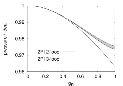
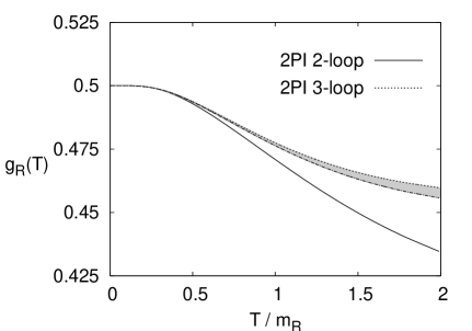
Figure 6: The left figure shows the results for pressure at a lower temperature ($T=m_{R}(0)$) than Fig. 1 as a function of the renormalized zero-temperature coupling. The right figure shows the renormalized thermal coupling as a function of temperature. As for Fig. 1 results are given employing two different renormalization scales. The shaded band indicates the renormalization scale dependence appearing at three-loop order.

In Fig. 6 we show results at a lower temperature, which is taken to be equal to the vacuum mass, i.e. $T=m_{R}$. We plot the pressure as a function of the vacuum coupling. This set of parameters has the feature that the thermal masses are within 1% equal in the two approximations for any coupling. In this case the three-loop curve is above the two-loop curve. Note that the two-loop contribution from the 2PI effective action is negative, while the three-loop correction is positive. This can be directly observed from the 2PI effective action before evaluation at the stationary point (2.4) for which $i\Gamma_{2}^{\rm 2loop}[\phi=0,D]\,T/L_{3}=-3g^{2}(\texttt{addup}\bar{D})^{2}$ and $i\Gamma_{2}^{\rm 3loop}[\phi=0,D]\,T/L_{3}=12(g_{R}/Z)^{4}\texttt{addup}(\bar{D}\texttt{fft}{\tilde{D}}^{3})$. As a consequence, if the propagators do not change much from two-loop to three-loop order then the pressure will always be increased by the three-loop contribution. On the right of Fig. 6 we also show the renormalized coupling as a function of temperature normalized to $m_{R}$.

For the exact theory the choice of a temperature scale for renormalization is irrelevant. However, for a given approximation the possible renormalization scale dependence of the results can be used as a check. The two-loop result is manifestly renormalization scale independent (cf. also Sec. 2.2). The three-loop results of Figs. 1 and 6 have been calculated first from renormalization at zero temperature and second from renormalization at a non-zero temperature $T=m_{R}$. The high-temperature renormalization conditions are chosen such that the results agree at zero temperature. At three loop this check is nontrivial because of the coupling dependence in Eq. (2.18) with $g_{R}=g_{R}(T=0)$ for the first calculation and $g_{R}=g_{R}(T=m_{R})$ for the second one. The variation of the thermal results of the two models give an idea about the scale dependence, which is indicated by the shaded bands in Fig. 6. A similar analysis employing different renormalization scales has been also performed for the 2PI three-loop results displayed on the left of Fig. 1. However, the difference between the results was hardly distinguishable in this high-temperature case. In contrast, the severe scale dependence of the perturbative calculations is well documented in the literature [10].

Compared to the perturbative expansions for pressure (cf. Fig. 1 right), our results indicate a substantially improved convergence for the 2PI expansions. This holds even for rather strong couplings. In our lattice calculations we approach the Landau pole with our momentum cutoff, i.e. we explore almost the full range of couplings principally available. The range of renormalized couplings for various lattice regularizations is shown in Fig. 7. For any momentum cutoff there is a highest value of $g_{R}$ for which there exists a bare coupling $g^{2}=g_{R}^{2}+\delta g^{2}$. (Cf. also the discussion for the two-loop effective action in Sec. 2.2.) Concerning the lattice discretization one gains precision by reducing the lattice spacing, however, the range of physical couplings that can be realized shrinks. From the comparison to the two-loop analytic formulae, and from three-loop calculations with a series of small lattice spacings, we infer that one should use $am_{R}(T_{0})\leq 0.125$ (for $T\leq 2m_{R}(T_{0})$, see Fig. 4). How this limits the available couplings to three-loop order is shown in Fig. 7.

Figure 7: Physical coupling ranges for different lattice spacings employing the three-loop 2PI effective action. Here we show the coupling counterterms $\delta g_{1}^{2}=\delta g_{2}^{2}$. The counterterms diverge at a certain value of the physical coupling.

Very similar techniques as those employed here can be straightforwardly used for more complicated systems, as for instance fermionic or Yukawa theories (cf. also Ref. [6]). A more ambitious generalization is the application of these techniques to gauge field theories. While linear symmetries as realized in QED can be treated along similar lines, the generalization to nonabelian gauge theories is technically more involved and needs to be further investigated [21].

Acknowledgements. We thank Jean-Paul Blaizot, Holger Gies, Edmond Iancu and Toni Rebhan for fruitful collaborations/discussions on these topics.

References

- [1] J. M. Luttinger and J. C. Ward, Phys. Rev. 118 (1960) 1417. G. Baym, Phys. Rev. 127 (1962) 1391. J. M. Cornwall, R. Jackiw and E. Tomboulis, Phys. Rev. D 10 (1974) 2428.
- [2] J. Berges and J. Cox, Phys. Lett. B 517 (2001) 369.
- [3] J. Berges, Nucl. Phys. A 699 (2002) 847.
- [4] For recent reviews see J. Berges and J. Serreau, “Progress in nonequilibrium quantum field theory”, in Strong and Electroweak Matter 2002, ed. M.G. Schmidt (World Scientific, 2003), http://arXiv:hep-ph/0302210 and “Progress in nonequilibrium quantum field theory II”, in Strong and Electroweak Matter 2004, Helsinki, 16-19 June 2004.
- [5] G. Aarts and J. Berges, Phys. Rev. D 64 (2001) 105010. S. Juchem, W. Cassing and C. Greiner, Phys. Rev. D 69 (2004) 025006.
- [6] J. Berges, S. Borsányi and J. Serreau, Nucl. Phys. B 660 (2003) 51. J. Berges, S. Borsányi and C. Wetterich, Phys. Rev. Lett. 93 (2004) 142002.
- [7] G. Aarts and J. Berges, Phys. Rev. Lett. 88 (2002) 041603. G. Aarts, D. Ahrensmeier, R. Baier, J. Berges and J. Serreau, Phys. Rev. D 66 (2002) 045008. J. Berges and J. Serreau, Phys. Rev. Lett. 91 (2003) 111601.
- [8] F. Cooper, J. F. Dawson and B. Mihaila, Phys. Rev. D 67 (2003) 056003. B. Mihaila, F. Cooper and J. F. Dawson, Phys. Rev. D 63 (2001) 096003.
- [9] E. Braaten and R. D. Pisarski, Nucl. Phys. B 337 (1990) 569. J. Frenkel and J. C. Taylor, Nucl. Phys. B 334 (1990) 199. J. C. Taylor and S. M. H. Wong, Nucl. Phys. B 346 (1990) 115.
- [10] J. P. Blaizot, E. Iancu and A. Rebhan, in “Quark Gluon Plasma 3”, eds. R.C. Hwa and X.N. Wang, World Scientific, Singapore, 60-122 [arXiv:hep-ph/0303185]. U. Kraemmer and A. Rebhan, Rept. Prog. Phys. 67 (2004) 351. J. O. Andersen and M. Strickland, arXiv:hep-ph/0404164.
- [11] J. P. Blaizot, E. Iancu and A. Rebhan, Phys. Rev. Lett. 83 (1999) 2906. Phys. Lett. B 470 (1999) 181. Phys. Rev. D 63 (2001) 065003.
- [12] B. Gruter, R. Alkofer, A. Maas and J. Wambach, arXiv:hep-ph/0408282.
- [13] E. Braaten and E. Petitgirard, Phys. Rev. D 65 (2002) 085039.
- [14] J. O. Andersen and M. Strickland, Phys. Rev. D 71 (2005) 025011.
- [15] The weak-coupling expansion of the pressure in the high temperature limit has been computed to order , first in P. Arnold and C.-X. Zhai, Phys. Rev. D 50 (1994) 7603. Perturbative results to three-loop order for the massive theory can be found in J. O. Andersen, E. Braaten and M. Strickland, Phys. Rev. D 62 (2000) 045004.
- [16] H. van Hees and J. Knoll, Phys. Rev. D 65 (2002) 025010. Phys. Rev. D 65 (2002) 105005. Phys. Rev. D 66 (2002) 025028.
- [17] J. P. Blaizot, E. Iancu and U. Reinosa, Phys. Lett. B 568 (2003) 160. Nucl. Phys. A 736 (2004) 149.
- [18] F. Cooper, B. Mihaila and J. F. Dawson, Phys. Rev. D 70 (2004) 105008.
- [19] A. Jakovác and Z. Szép, arXiv:hep-ph/0405226. H. Verschelde and J. De Pessemier, Eur. Phys. J. C 22 (2002) 771.
- [20] J. Baacke and A. Heinen, Phys. Rev. D 68 (2003) 127702.
- [21] J. Berges, Sz. Borsányi, U. Reinosa and J. Serreau, hep-ph/0503240
- [22] J. Berges, Phys. Rev. D 70 (2004) 105010.
- [23] C. De Dominicis and P. C. Martin, J. Math. Phys. 5 (1964) 14, 31. R.E. Norton and J.M. Cornwall, Ann. Phys. (N.Y.) 91 (1975) 106. H. Kleinert, Fortschritte der Physik 30 (1982) 187. A.N. Vasiliev, “Functional Methods in Quantum Field Theory and Statistical Physics”, Gordon and Breach Science Pub. (1998).
- [24] E. Calzetta and B. L. Hu, Phys. Rev. D 37 (1988) 2878. Phys. Rev. D 61 (2000) 025012.
- [25] M. Alford, J. Berges and J. M. Cheyne, Phys. Rev. D 70 (2004) 125002.
- [26] I. T. Drummond, R. R. Horgan, P. V. Landshoff and A. Rebhan, Nucl. Phys. B 524 (1998) 579.
- [27] M. Lüscher and P. Weisz, Nucl. Phys. B 290 (1987) 25.