Systematic limits on $\sin^{2}{2\theta_{13}}$ in neutrino oscillation experiments with multi-reactors

Abstract

Sensitivities to $\sin^{2}{2\theta_{13}}$ without statistical errors (“systematic limit”) are investigated in neutrino oscillation experiments with multiple reactors. Using an analytical approach, we show that the systematic limit on $\sin^{2}{2\theta_{13}}$ is dominated by the uncorrelated systematic error $\sigma_{\text{u}}$ of the detector. Even in an experiment with multi-detectors and multi-reactors, it turns out that most of the systematic errors including the one due to the nature of multiple sources is canceled as in the case with a single reactor plus two detectors, if the near detectors are placed suitably. The case of the KASKA plan (7 reactors and 3 detectors) is investigated in detail, and it is explicitly shown that it does not suffer from the extra uncertainty due to multiple reactors.

I Introduction

Recently the possibility to measure $\theta_{13}$ by a reactor experiment has attracted much attention kr2det ; Minakata:2002jv ; Huber:2003pm ; kaska ; Ardellier:2004ui ; Shaevitz:2003ws ; USreactor ; Daya ; Anderson:2004pk . To achieve sensitivity $\sin^{2}{2\theta_{13}}\sim 0.01$, reduction of the systematic errors is crucial, and near and far detectors seem to be necessary for that purpose. On the other hand, it appears to be advantageous to do an experiment at a multi-reactor site to gain statistics and high signal to noise ratio, and in fact in the most of cases considered in kr2det ; Minakata:2002jv ; Huber:2003pm ; kaska ; Ardellier:2004ui ; Shaevitz:2003ws ; USreactor ; Daya ; Anderson:2004pk there are more than one reactor. In this paper we discuss the systematic errors in reactor neutrino oscillation experiments with multi reactors and multi detectors in an analytical way. In Sect.2 we discuss the cases with a single reactor to illustrate our analytical method. In Sect.3 we consider the cases with $n_{r}$ reactors and show that the larger $n_{r}$ gives totally the smaller contribution to the sensitivity from the uncorrelated errors of the fluxes. Irrespective of the number of reactors, if there are more than one detectors, we can cancel the correlated errors which includes the error of the fluxes. We emphasize in this paper that the sensitivity on $\sin^{2}{2\theta_{13}}$ with vanishing statistical errors (we refer to the sensitivity as the systematic limit) is dominated by the uncorrelated error of the detectors in most cases. It is also emphasized that a lot of caution has to be exercised to estimate the uncorrelated error. In the appendix we give some details on how to derive the analytic results used in the main text, using the equivalence of the pull method and the covariance matrix approach Stump:2001gu ; Botje:2001fx ; Pumplin:2002vw ; Fogli:2002pt . Throughout this paper we do not use the binning of the numbers of events because the discussions on the uncorrelated bin-to-bin systematic errors are complicated. Also we will discuss only the systematic errors, i.e., we will consider the case where the statistical errors are negligibly small.

II Systematic errors

To discuss the systematic limit on $\sin^{2}{2\theta_{13}}$ in neutrino oscillation experiments with multiple reactors, we have to introduce the systematic errors of the detectors and the reactors (fluxes). There are two kinds of systematic errors of the detectors, namely, the correlated error $\sigma_{c}$ and uncorrelated error $\sigma_{u}$. The former includes the theoretical uncertainty in the cross section of detection, etc. while the latter does the uncertainty in the baseline lengths, a portion of measuring the detector volume, a part of the detection efficiency, etc. As for the systematic errors of the reactors (fluxes), the correlated error $\sigma^{(r)}_{c}$ consists of the uncertainties in the spectrum of the $\overline{\nu}_{e}$ flux, etc. whereas the uncorrelated error $\sigma^{(r)}_{u}$ consists of the uncertainties in the composition of the fuel, etc. In this paper we adopt the reference values for $\sigma_{\text{c}}$ and $\sigma_{\text{u}}$ used in Minakata:2002jv , where basically the same reference values as in the Bugey experiment Declais:1994su were assumed. $\sigma_{\text{c}}$ and $\sigma_{\text{u}}$ can be estimated to be

$$\sigma_{\text{u}} = 0.8\%/\sqrt{2}=0.6\%$$

$$\sigma_{\text{c}} = \sqrt{(2.7\%)^{2}-(2.1\%)^{2}-(0.8\%/\sqrt{2})^{2}}=1.6\%,$$ (1)

where the factor $\sqrt{2}$ appears because the relative normalization $\sigma_{\text{rel}}$=0.8% in Declais:1994su is related to $\sigma_{\text{u}}$ by $\sigma_{\text{rel}}=\sqrt{2}\sigma_{\text{u}}$. In the estimation of $\sigma_{\text{c}}$, we used 2.7% total error and 2.1% error of the flux which are the values in the CHOOZ experiment. As for the correlated and uncorrelated errors of the the flux from the reactors, we adopt the same reference values as those used by the KamLAND experiment Eguchi:2002dm

$$\sigma_{\text{c}}^{\text{(r)}} = 2.5\%,$$

$$\sigma_{\text{u}}^{\text{(r)}} = 2.3\%.$$ (2)

Note that the word “correlated” means just the type of the error, and then correlated errors exist even if there is no partner.

III One reactor

To explain our analytical approach, let us start with the simplest case, namely the case with one reactor.

III.1 One detector

Let $m$ be the measured number of events at the detector, $t$ be the theoretical predictions (hypothesis) to be tested. $\chi^{2}$ is defined as

$$\displaystyle\chi^{2} = \min_{\alpha^{\prime}s}\left\{\left[{m-t(1+\alpha_{\text{c}}+\alpha_{\text{c}}^{\text{(r)}}+\alpha_{\text{u}}^{(r)})\over t\sigma_{\text{u}}}\right]^{2}+\left({\alpha_{\text{c}}\over\sigma_{\text{c}}}\right)^{2}+\left({\alpha_{\text{c}}^{\text{(r)}}\over\sigma_{\text{c}}^{\text{(r)}}}\right)^{2}+\left({\alpha_{\text{u}}^{\text{(r)}}\over\sigma_{\text{u}}^{\text{(r)}}}\right)^{2}\right\}$$ (3)

$$= {\left(\displaystyle{m\over t}-1\right)^{2}\over\sigma_{\text{u}}^{2}+\sigma_{\text{c}}^{2}+(\sigma_{\text{c}}^{\text{(r)}})^{2}+(\sigma_{\text{u}}^{\text{(r)}})^{2}},$$

where $\alpha_{u}$, $\alpha_{c}$, $\alpha^{(r)}_{c}$ and $\alpha^{(r)}_{u}$ are the variables of noises to introduce the systematic errors $\sigma_{u}$, $\sigma_{c}$, $\sigma^{(r)}_{c}$ and $\sigma^{(r)}_{u}$, respectively. We give an easier way to derive (3) in the Appendix A, where integration over the $\alpha$ variables as those of Gaussian, instead of minimizing with respect to these variables, do the same job. Eq. (3) shows that the square of the total systematic error is given by the sum of the squares of all the systematic errors.

Our strategy in this paper is to assume no neutrino oscillation for the theoretical predictions $t$’s and assume the number of events with oscillations for the measured values $m$’s. Then, we examine whether a hypothesis with no oscillation is excluded or not, say at the 90%CL, from the value of $\chi^{2}$. In the context of neutrino oscillation experiments, we have

$$\displaystyle{m\over t}-1=-\sin^{2}2\theta\left\langle\sin^{2}\left({\Delta m^{2}L\over 4E}\right)\right\rangle$$ (4)

in the two flavor framework, where $\theta$ is the mixing angle, $\Delta m^{2}$ is the mass squared difference, $E$ is the neutrino energy, $L$ is the distance of the reactor and the detector, and

$$\displaystyle\left\langle\sin^{2}\left({\Delta m^{2}L_{j}\over 4E}\right)\right\rangle\equiv{\displaystyle\int dE~{}\epsilon(E)f(E)\sigma(E)\sin^{2}\left({\Delta m^{2}L_{j}\over 4E}\right)\over\displaystyle\int dE~{}\epsilon(E)f(E)\sigma(E)}.$$

$\epsilon(E)$, $f(E)$, $\sigma(E)$ stand for the detection efficiency, the neutrino flux, and the cross section, respectively.

III.2 Two detectors

Next let us discuss a less trivial example with a single reactor, one near and one far detectors. Let $m_{\text{n}}$ and $m_{\text{f}}$ be the measured numbers of events at the near and far detectors, $t_{\text{n}}$ and $t_{\text{f}}$ be the theoretical predictions, respectively. Then $\chi^{2}$ is given by

$$\displaystyle\chi^{2} = \min_{\alpha^{\prime}s}\left\{\left[{m_{\text{n}}-t_{\text{n}}(1+\alpha_{\text{c}}+\alpha_{\text{c}}^{\text{(r)}}+\alpha_{\text{u}}^{(r)})\over t_{\text{n}}\sigma_{\text{u}}}\right]^{2}+\left[{m_{\text{f}}-t_{\text{f}}(1+\alpha_{\text{c}}+\alpha_{\text{c}}^{\text{(r)}}+\alpha_{\text{u}}^{(r)})\over t_{\text{f}}\sigma_{\text{u}}}\right]^{2}\right.$$ (5)

$$\left.+\left({\alpha_{\text{c}}\over\sigma_{\text{c}}}\right)^{2}+\left({\alpha_{\text{c}}^{\text{(r)}}\over\sigma_{\text{c}}^{\text{(r)}}}\right)^{2}+\left({\alpha_{\text{c}}^{\text{(r)}}\over\sigma_{\text{c}}^{\text{(r)}}}\right)^{2}\right\},$$

where we have assumed that the uncorrelated errors for the two detectors are the same and are equal to $\sigma_{\text{u}}$. Eq. (5) can be evaluated also by integrating over the variables $\alpha_{\text{c}}$, etc. as Gaussian instead of minimizing with respect to these variables. After some calculations (See Appendix A for details), we obtain

$$\displaystyle\chi^{2}=\left(\begin{array}[]{cc}\displaystyle{m_{\text{n}}\over t_{\text{n}}}-1,&\displaystyle{m_{\text{f}}\over t_{\text{f}}}-1\end{array}\right)V^{-1}\left(\begin{array}[]{c}\displaystyle{m_{\text{n}}\over t_{\text{n}}}-1\\ \\ \displaystyle{m_{\text{f}}\over t_{\text{f}}}-1\end{array}\right),$$ (10)

where

$$V \equiv \sigma^{2}_{\text{u}}\,I_{2}+\left[\sigma^{2}_{\text{c}}+(\sigma^{\text{(r)}}_{\text{u}})^{2}+(\sigma^{\text{(r)}}_{\text{c}})^{2}\right]H_{2}$$ (13)

$$= \left(\displaystyle\begin{array}[]{rr}\sigma^{2}_{\text{u}}+\sigma^{2}_{\text{c}}+(\sigma^{\text{(r)}}_{\text{u}})^{2}+(\sigma^{\text{(r)}}_{\text{c}})^{2}&\quad\sigma^{2}_{\text{c}}+(\sigma^{\text{(r)}}_{\text{u}})^{2}+(\sigma^{\text{(r)}}_{\text{c}})^{2}\\[8.53581pt] \quad\sigma^{2}_{\text{c}}+(\sigma^{\text{(r)}}_{\text{u}})^{2}+(\sigma^{\text{(r)}}_{\text{c}})^{2}&\sigma^{2}_{\text{u}}+\sigma^{2}_{\text{c}}+(\sigma^{\text{(r)}}_{\text{u}})^{2}+(\sigma^{\text{(r)}}_{\text{c}})^{2}\end{array}\right)$$

is the covariance matrix; $I_{2}$ represents $2\times 2$ identity matrix and $H_{2}$ does a $2\times 2$ matrix whose elements are all unity. It is seen that only the covariant matrix in the $\chi^{2}$ depends on the errors. Note that any liner transformation of $V$ does not change the value of $\chi^{2}$. Diagonalization of $V$ is, however, worthwhile to investigate analytically the behavior of $\chi^{2}$. After diagonalizing $V$ we have

$$\displaystyle\chi^{2} = {\left[\left(m_{\text{n}}/t_{\text{n}}-1\right)+\left(m_{\text{f}}/t_{\text{f}}-1\right)\right]^{2}\over 4\sigma^{2}_{\text{c}}+4(\sigma^{\text{(r)}}_{\text{u}})^{2}+4(\sigma^{\text{(r)}}_{\text{c}})^{2}+2\sigma^{2}_{\text{u}}}+{\left[\left(m_{\text{n}}/t_{\text{n}}-1\right)-\left(m_{\text{f}}/t_{\text{f}}-1\right)\right]^{2}\over 2\sigma^{2}_{\text{u}}}$$ (14)

$$= \sin^{4}2\theta\left[{\left(D(L_{\text{f}})+D(L_{\text{n}})\right)^{2}\over 4\sigma^{2}_{\text{c}}+4(\sigma^{\text{(r)}}_{\text{u}})^{2}+4(\sigma^{\text{(r)}}_{\text{c}})^{2}+2\sigma^{2}_{\text{u}}}+{\left(D(L_{\text{f}})-D(L_{\text{n}})\right)^{2}\over 2\sigma^{2}_{\text{u}}}\right],$$ (15)

where $L_{\text{n}}$ and $L_{\text{f}}$ are the distances from the reactor to the near and far detector, respectively; We have defined

$$\displaystyle D(L)\equiv\left\langle\sin^{2}\left({\Delta m^{2}L\over 4E}\right)\right\rangle.$$ (16)

The first term on the right hand side in Eq. (14) stands for the contribution from the sum of the yields at the near and far detectors, while the second term corresponds to the difference between them. The first term determines the normalization of flux, namely the sensitivity on $\sin^{2}{2\theta}$ at very large $|\Delta m^{2}|$ where all $D(L)$ becomes $0.5\sin^{2}{2\theta}$. On the other hand, the second term gives the main sensitivity at the concerned value of $|\Delta m^{2}|$ (e.g. $2.5\times 10^{-3}\text{eV}^{2}$) as we see below.

Putting the reference values (1) and (2) together, we have

$$2\sigma_{\text{u}}^{2} = (0.8\%)^{2},$$

$$4\sigma_{\text{c}}^{2}+4(\sigma^{\text{(r)}}_{\text{u}})^{2}+4(\sigma^{\text{(r)}}_{\text{c}})^{2}+2\sigma_{\text{u}}^{2} = (7.6\%)^{2}.$$

We can ignore the contribution from $(4\sigma_{\text{c}}^{2}+4(\sigma^{\text{(r)}}_{\text{u}})^{2}+4(\sigma^{\text{(r)}}_{\text{c}})^{2}+2\sigma_{\text{u}}^{2})^{-1}$ in Eq. (15) because that is only 1% compared to that from $(2\sigma_{\text{u}}^{2})^{-1}$. Hence, $\chi^{2}$ is given approximately by

$$\chi^{2}\simeq\sin^{4}2\theta{\left(D(L_{\text{f}})-D(L_{\text{n}})\right)^{2}\over 2\sigma^{2}_{\text{u}}}.$$ (17)

We see that the main sensitivity is determined indeed by the relative normalization error $\sigma_{\text{rel}}=\sqrt{2}\sigma_{\text{u}}$. By comparing (3) and (17), it is clear that the sensitivity is improved significantly by virtue of near detector. The hypothesis of no oscillation is excluded at the 90%CL if $\chi^{2}$ is larger than 2.7, which corresponds to the value at the 90%CL for one degree of freedom. This implies that the systematic limit on $\sin^{2}2\theta$ at the 90%CL, namely the sensitivity in the limit of infinite statistics, is given by

$$\left(\sin^{2}2\theta\right)_{\text{limit}}^{\text{sys~{}only}}\simeq\sqrt{2.7}{\sqrt{2}\sigma_{\text{u}}\over D(L_{\text{f}})-D(L_{\text{n}})}.$$ (18)

Eq. (18) also tells us that, in order to optimize $\left(\sin^{2}2\theta\right)_{\text{limit}}^{\text{sys~{}only}}$ for a given value of $\sigma_{\text{u}}$, we have to maximize $D(L_{\text{f}})\equiv\langle\sin^{2}\left({\Delta m^{2}L_{\text{f}}/4E}\right)\rangle$ while minimizing $D(L_{\text{n}})\equiv\langle\sin^{2}\left({\Delta m^{2}L_{\text{n}}/4E}\right)\rangle$. Note that $D(L_{\text{f}})$ can not be unity because of neutrino energy spectrum; The possible maximum value of $D(L_{\text{f}})-D(L_{\text{n}})$ is 0.82, which is attained for $\Delta m^{2}=2.5\times 10^{-3}\text{eV}^{2}$, $L_{\text{f}}=1.8$km, and $L_{\text{n}}=0$. Then, we can estimate the lower bound of $\left(\sin^{2}2\theta\right)_{\text{limit}}^{\text{sys~{}only}}$ at a single reactor experiment, assuming that the uncorrelated error $\sigma_{\text{u}}$ is smaller enough than other errors:

$$\left(\sin^{2}2\theta\right)_{\text{limit}}^{\text{sys~{}only}}\gtrsim{\sqrt{2.7}\sqrt{2}\sigma_{\text{u}}\over 0.82}=2.8\,\sigma_{\text{u}}.$$ (19)

In practice, however, $D(L_{\text{n}})$ will not be able to vanish. Assuming $\Delta m^{2}=2.5\times 10^{-3}\text{eV}^{2}$, $L_{\text{f}}=1.7\text{km}$, and $L_{\text{n}}=0.3\text{km}$, we have $D(L_{\text{f}})\simeq 0.82$ and $D(L_{\text{n}})\simeq 0.07$. Then, $\sigma_{\text{u}}=(0.8/\sqrt{2})\%$ gives the sensitivity

$$\left(\sin^{2}2\theta\right)_{\text{limit}}^{\text{sys~{}only}}\simeq\sqrt{2.7}{\sqrt{2}\sigma_{\text{u}}\over D(L_{\text{f}})-D(L_{\text{n}})}\simeq 3.1\sigma_{\text{u}}\simeq 0.018.$$

This sensitivity corresponds to and agrees with the value obtained numerically in Minakata:2002jv .

IV $n_{r}$ reactors

It is straightforward to generalize the argument in the previous section to a general case with multi-reactors and multi-detectors. The covariance matrix $V$ is given by $\sigma_{\text{u}}^{2}\times$(unit matrix)+(the rest), and in most cases, as long as the near detectors are placed properly, the determinant of (the rest) is zero or very small compared to $\sigma_{\text{u}}^{2}$. The minimum eigenvalue of the covariance matrix, which gives main contribution to $\chi^{2}$, is approximately given by $\sigma_{\text{u}}^{2}$. Therefore, the systematic limit is dominated by the uncorrelated error $\sigma_{\text{u}}$ also in general cases.

IV.1 One detector

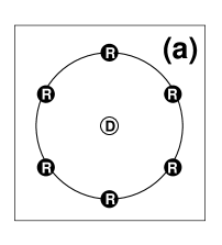
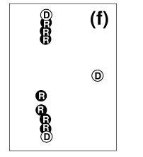
As in Sect. III, as a warming up, let us consider the case with one detector and multiple reactors (See Fig.1(a)). When there are $n_{r}(>1)$ reactors, the total number $m$ of the measured events is a sum of contributions $m_{a}~{}(a=1,\cdots,n_{r})$ from each reactor, and this is also the case for the theoretical predictions $t$ and $t_{a}~{}(a=1,\cdots,n_{r})$. So we have

$$m=\sum_{a=1}^{n_{r}}m_{a},\quad t=\sum_{a=1}^{n_{r}}t_{a}.$$

Taking these systematic errors into consideration, the total number $t$ of the theoretical prediction is redefined as

$$t \rightarrow \sum_{a=1}^{n_{r}}t_{a}\left(1+\alpha_{\text{c}}+\alpha_{\text{c}}^{\text{(r)}}+\alpha_{\text{u}a}^{(r)}\right)$$

$$= t\left(1+\alpha_{\text{c}}+\alpha_{\text{c}}^{\text{(r)}}\right)+\sum_{a=1}^{n_{r}}t_{a}\alpha_{\text{u}a}^{(r)}=t\left(1+\alpha_{\text{c}}+\alpha_{\text{c}}^{\text{(r)}}+\sum_{a=1}^{n_{r}}{t_{a}\over t}\alpha_{\text{u}a}^{(r)}\right),$$

where $\alpha_{\text{u}a}^{(r)}$ is the variable to introduce the uncorrelated of the flux from the $a$-th reactor. $\chi^{2}$ is defined as

$$\chi^{2} = \min_{\alpha^{\prime}s}\left\{{1\over t^{2}\sigma^{2}}\left[m-t\left(1+\alpha_{\text{c}}+\alpha_{\text{c}}^{\text{(r)}}+\sum_{a=1}^{n_{r}}{t_{a}\over t}\alpha_{\text{u}a}^{\text{r}}\right)\right]^{2}\right.$$

$$\left.+\left({\alpha_{\text{c}}\over\sigma_{\text{c}}}\right)^{2}+\left({\alpha_{\text{c}}^{\text{(r)}}\over\sigma_{\text{c}}^{\text{(r)}}}\right)^{2}+\sum_{a=1}^{n_{r}}\left({\alpha_{\text{u}a}^{\text{(r)}}\over\sigma_{\text{u}}^{\text{(r)}}}\right)^{2}\right\},$$

where we have again assumed for simplicity that the size of the uncorrelated error in the flux from the reactors is common: $\sigma_{\text{u}a}^{\text{(r)}}=\sigma_{\text{u}}^{\text{(r)}}$. Performing minimization with respect to the $\alpha$ variables, we get (See Appendix A)

$$\chi^{2}={\left(\displaystyle{m\over t}-1\right)^{2}\over\displaystyle\sigma_{\text{u}}^{2}+\sigma_{\text{c}}^{2}+(\sigma_{\text{c}}^{\text{(r)}})^{2}+(\sigma_{\text{u}}^{\text{(r)}})^{2}\sum_{a=1}^{n_{r}}\left({t_{a}\over t}\right)^{2}}.$$ (20)

By comparing (20) with (3), we find that the multiple reactor nature affects $\chi^{2}$ (the sensitivity on $\sin^{2}2\theta$) through $\sigma_{\text{u}}^{\text{(r)}}$. Since there is only one detector in this case, the correlated error was not canceled in $\chi^{2}$ and it contributes to the systematic limit on $\sin^{2}2\theta$. However, if the yield from each reactor is approximately equal, i.e., if

$${t_{a}\over t}\simeq{1\over n_{r}},$$ (21)

then the contribution of the uncorrelated error of the reactors becomes

$$(\sigma_{\text{u}}^{\text{(r)}})^{2}\sum_{a=1}^{n_{r}}\left({t_{a}\over t}\right)^{2}\simeq\displaystyle{1\over n_{r}}(\sigma_{\text{u}}^{\text{(r)}})^{2}.$$ (22)

Comparing Eqs. (3) and (20), we observe that the contribution of the uncorrelated error of the reactors decreases as the number of the reactors increases, as long as the condition (22) is satisfied. This is because the average of independent $n_{r}$ fluctuations is smaller than a single fluctuation.

IV.2 $n_{d}$ detectors

Let us now discuss more general cases with $n_{r}$ reactors and $n_{d}$ detectors. For simplicity we assume again that the size of the uncorrelated errors for the detectors are the same and the size of the uncorrelated errors in the flux from the reactors are also the same: $\sigma_{\text{u}j}=\sigma_{\text{u}}$, $\sigma_{\text{u}a}^{(\text{r})}=\sigma_{\text{r}}^{\text{u}}$. Let $t_{ja}$ ($m_{ja}$) be the theoretical prediction (measured value) for the number of events of neutrinos from the $a$-th reactor $(a=1,\cdots,n_{r})$ at the $j$-th detector $(j=1,\cdots,n_{d})$ and $t_{j}=\sum_{a=1}^{n_{r}}t_{ja}$ ($m_{j}=\sum_{a=1}^{n_{r}}m_{ja}$) be the theoretical (measured) total number of events at the $j$-th detector. Then generalizing the discussions in the previous sections, we have

$$\chi^{2} = \min_{\alpha^{\prime}s}\left\{\displaystyle\sum_{j=1}^{n_{d}}{1\over t_{j}^{2}\sigma_{\text{u}}^{2}}\left[m_{j}-t_{j}\left(1+\alpha_{\text{c}}+\alpha_{\text{c}}^{\text{(r)}}+\sum_{a=1}^{n_{r}}{t_{aj}\over t_{j}}\alpha_{\text{u}a}^{(r)}\right)\right]^{2}\right.$$

$$+\left.\left({\alpha_{\text{c}}\over\sigma_{\text{c}}}\right)^{2}+\left({\alpha_{\text{c}}^{\text{(r)}}\over\sigma_{\text{c}}^{\text{(r)}}}\right)^{2}+\sum_{a=1}^{n_{r}}\left({\alpha_{\text{u}a}^{\text{(r)}}\over\sigma_{\text{u}}^{\text{(r)}}}\right)^{2}\right\}.$$

After some calculation (See Appendix A), we have

$$\chi^{2} = \left(\displaystyle{m_{1}\over t_{1}}-1,\cdots,\displaystyle{m_{n_{d}}\over t_{n_{d}}}-1\right)V^{-1}\left(\begin{array}[]{c}\displaystyle{m_{1}\over t_{1}}-1\\ \vdots\\ \displaystyle{m_{n_{d}}\over t_{n_{d}}}-1\end{array}\right),$$ (26)

where

$$V_{jk} = \delta_{jk}\sigma_{\text{u}}^{2}+\sigma_{\text{c}}^{2}+(\sigma_{\text{c}}^{\text{(r)}})^{2}+(\sigma_{\text{u}}^{\text{(r)}})^{2}\displaystyle\sum_{a=1}^{n_{r}}\displaystyle{t_{aj}\over t_{j}}{t_{ak}\over t_{k}}.$$ (27)

IV.2.1 $n_{r}$ reactors and $(n_{r}+1)$ detectors

In Sect. III we have seen that the correlated error is canceled in the case of a single reactor experiment with one near and one far detectors. Now we would like to ask the following question: what happens to this cancellation in the case of an experiment with multiple reactors and detectors? To answer this question, let us consider the ideal case with $n_{r}$ reactors and $(n_{r}+1)$ detectors, where each reactor has a near detector in its neighborhood and each reactor produces the same number of events at a far detector (See Fig.1(b)):

$$\mbox{\rm near detectors}:~{} \displaystyle{t_{aj}\over t_{j}}=\delta_{aj}~{}\qquad\quad(j=1,\cdots,n_{r};a=1,\cdots,n_{r})$$ (28)

$$\mbox{\rm far detector}:~{} \displaystyle{t_{a\,n_{r}+1}\over t_{n_{r}+1}}=\displaystyle{1\over n_{r}}\qquad(a=1,\cdots,n_{r}).$$

In this case the element of the covariance matrix becomes

$$V = \sigma_{\text{u}}^{2}\,I_{n_{r}+1}+\left[\sigma_{\text{c}}^{2}+\left(\sigma_{\text{c}}^{(r)}\right)^{2}\right]H_{n_{r}+1}+\left(\sigma_{\text{u}}^{(r)}\right)^{2}\left(\begin{array}[]{ccccc}1&0&\cdots&0&1/n_{r}\\ 0&\ddots&&\vdots&\vdots\\ \vdots&&\ddots&0&\vdots\\ 0&\cdots&0&1&\vdots\\[8.53581pt] 1/n_{r}&\cdots&\cdots&\cdots&1/n_{r}\end{array}\right),$$ (34)

where $I_{n_{r}+1}$ is an $(n_{r}+1)\times(n_{r}+1)$ unit matrix, and $H_{n_{r}+1}$ is an $(n_{r}+1)\times(n_{r}+1)$ matrix defined by

$$H_{n_{r}+1} \equiv \left(\begin{array}[]{ccc}1&\cdots&1\\ \vdots&&\vdots\\ 1&\cdots&1\end{array}\right).$$ (38)

Here we assume the following conditions:

$$\left|{\Delta m^{2}L_{\text{n}}\over 4E}\right|\ll 1,\ \ \ \left|{\Delta m^{2}L_{\text{f}}\over 4E}\right|\simeq{\pi\over 2}.$$ (39)

These conditions have to be satisfied in an experiment which aims to measure $\theta_{13}$. From Eqs. (39) we have

$$\left(\begin{array}[]{c}m_{1}/t_{1}-1\\ \vdots\\ m_{n_{r}}/t_{n_{r}}-1\\ m_{n_{r}+1}/t_{n_{r}+1}-1\\ \end{array}\right)\simeq\left(\begin{array}[]{c}0\\ \vdots\\ 0\\ -\sin^{2}2\theta\left\langle\sin^{2}\left(\displaystyle{\Delta m^{2}L_{\text{f}}\over 4E}\right)\right\rangle\\ \end{array}\right)\equiv-\sin^{2}2\theta D(L_{\text{f}})\left(\begin{array}[]{c}0\\ \vdots\\ 0\\ 1\end{array}\right),$$ (52)

and $\chi^{2}$ becomes (See appendix B for derivation.)

$$\chi^{2}=\sin^{4}2\theta D(L_{\text{f}})^{2}\left\{{1\over n_{r}+1}{1\over\sigma_{\text{u}}^{2}+(n_{r}+1)\left[\sigma_{\text{c}}^{2}+\left(\sigma_{\text{c}}^{(r)}\right)^{2}+\left(\sigma_{\text{u}}^{(r)}\right)^{2}/n_{r}\right]}+{n_{r}\over n_{r}+1}{1\over\sigma_{\text{u}}^{2}}\right\}.$$ (53)

Then, the systematic limit on $\sin^{2}2\theta$ at the 90%CL is given by

$$\left(\sin^{2}2\theta\right)_{\text{limit}}^{\text{sys~{}only}}$$

$$=\sqrt{2.7}\sqrt{1+\displaystyle{1\over n_{r}}}\,{\sigma_{\text{u}}\over D(L_{\text{f}})}\,\left\{1+{\sigma_{\text{u}}^{2}/n_{r}\over\sigma_{\text{u}}^{2}+(n_{r}+1)\left[\sigma_{\text{c}}^{2}+\left(\sigma_{\text{c}}^{(r)}\right)^{2}+\left(\sigma_{\text{u}}^{(r)}\right)^{2}/n_{r}\right]}\right\}^{-\displaystyle{1\over 2}}$$ (54)

$$\simeq\sqrt{2.7}\sqrt{1+\displaystyle{1\over n_{r}}}\,{\sigma_{\text{u}}\over D(L_{\text{f}})}.$$ (55)

For example, we obtain $\left(\sin^{2}2\theta\right)_{\text{limit}}^{\text{sys~{}only}}\simeq 0.012$ by assuming seven reactors, $L_{\text{f}}=1.7\text{km}$, and $\sigma_{\text{u}}=0.8/\sqrt{2}\%$. As in the case with one reactor, the dominant contribution to the systematic limit comes from the uncorrelated error $\sigma_{\text{u}}$. The contribution of the uncorrelated error of flux, $\sigma^{(r)}_{\text{u}}$, is reduced in (54) by a factor of $n_{r}$ due to the averaging over the independent $n_{r}$ fluctuations; Although this reduction is a potential merit of the multiple reactor complex, it is irrelevant to the sensitivity because such an effect comes in the correlated error among detectors which is almost canceled in the multi-detector system. The factor $\sqrt{1+1/n_{r}}$ which appears in the dominant contribution by $\sigma_{\text{u}}$ indicates that the effective systematic error decreases as the number $(1+n_{r})$ of the detectors increases, since more information is obtained with more detectors. To conclude, the answer to the question at the beginning of this subsection is that the cancellation of the correlated error occurs also in the ideal case with $n_{r}$ reactors and $(n_{r}+1)$ detectors, and once again the systematic limit is dominated by $\sigma_{\text{u}}$. It should be noted that the number $n_{r}$ of the near detectors in this case is sufficient but not necessary to guarantee this cancellation, as we will see below in the case of the KASKA plan.

IV.2.2 The case of the KASKA plan

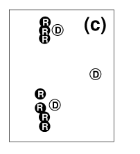
The Kashiwazaki-Kariwa nuclear power station consists of two clusters of reactors, and one cluster consists of four reactors while the other consists of three (See Fig.1(c)). According to the discussion in the previous section, we understand that near-far cancellation occurs for the KASKA case if we have seven near detectors. In the KASKA plan, however, not each reactors but each cluster of reactors assumed to have a near detector. In this subsection we would like to clarify the following questions on the KASKA plan kaska : (a) Is the number of near detectors sufficient for the cancellation of the correlated error? (b) What are the effects of multiple sources? (c) Is the KASKA plan optimized with respect to the sensitivity to $\sin^{2}2\theta$? Here we again assume that the size of the uncorrelated error in the flux from the reactors is common and the size of the uncorrelated errors of the three detectors are the same.

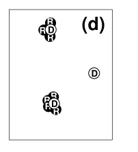
Before we discuss the systematic limit for the actual KASKA plan, let us consider the ideal limit, in which all the reactors in each cluster shrinks to one point as is shown in Fig.1(d); The ideal limit is similar to the case discussed in the section IV.2.1, namely the case of two reactors and three detectors. In this ideal limit, we have

$$\mbox{\rm near 1:}\qquad\displaystyle{t_{a1}\over t_{1}} = \left\{\begin{array}[]{cc}\displaystyle\frac{1}{\,4\,}&\qquad(a=1,\cdots,4)\\[14.22636pt] 0&\qquad(a=5,6,7)\end{array}\right.$$ (58)

$$\mbox{\rm near 2:}\qquad\displaystyle{t_{a2}\over t_{2}} = \left\{\begin{array}[]{cc}0&\qquad(a=1,\cdots,4)\\[8.53581pt] \displaystyle\frac{1}{\,3\,}&\qquad(a=5,6,7)\end{array}\right.$$ (61)

$$\mbox{\rm far:}\qquad\displaystyle{t_{a3}\over t_{3}} = \displaystyle\frac{1}{\,7\,}\qquad(a=1,\cdots,7)$$ (62)

and the covariance matrix is given by

$$V = \sigma_{\text{u}}^{2}I_{3}+\left[\sigma_{\text{c}}^{2}+\left(\sigma_{\text{c}}^{(r)}\right)^{2}\right]H_{3}+\left(\sigma_{\text{u}}^{(r)}\right)^{2}\left(\begin{array}[]{ccc}1/4&0&1/7\\ 0&1/3&1/7\\ 1/7&1/7&1/7\end{array}\right)$$ (66)

$$= \left(\begin{array}[]{lll}\sigma^{2}_{\text{c}}+(\sigma^{\text{(r)}}_{\text{c}})^{2}+\displaystyle{(\sigma_{\text{u}}^{\text{(r)}})^{2}\over 4}+\sigma^{2}_{\text{u}}&\quad\sigma^{2}_{\text{c}}+(\sigma^{\text{(r)}}_{\text{c}})^{2}&\quad\sigma^{2}_{\text{c}}+(\sigma^{\text{(r)}}_{\text{c}})^{2}+\displaystyle{(\sigma_{\text{u}}^{\text{(r)}})^{2}\over 7}\\[8.53581pt] \sigma^{2}_{\text{c}}+(\sigma^{\text{(r)}}_{\text{c}})^{2}&\quad\sigma^{2}_{\text{c}}+(\sigma^{\text{(r)}}_{\text{c}})^{2}+\displaystyle{(\sigma_{\text{u}}^{\text{(r)}})^{2}\over 3}+\sigma^{2}_{\text{u}}&\quad\sigma^{2}_{\text{c}}+(\sigma^{\text{(r)}}_{\text{c}})^{2}+\displaystyle{(\sigma_{\text{u}}^{\text{(r)}})^{2}\over 7}\\[8.53581pt] \sigma^{2}_{\text{c}}+(\sigma^{\text{(r)}}_{\text{c}})^{2}+\displaystyle{(\sigma_{\text{u}}^{\text{(r)}})^{2}\over 7}&\quad\sigma^{2}_{\text{c}}+(\sigma^{\text{(r)}}_{\text{c}})^{2}+\displaystyle{(\sigma_{\text{u}}^{\text{(r)}})^{2}\over 7}&\quad\sigma^{2}_{\text{c}}+(\sigma^{\text{(r)}}_{\text{c}})^{2}+\displaystyle{(\sigma_{\text{u}}^{\text{(r)}})^{2}\over 7}+\sigma^{2}_{\text{u}}\end{array}\right),$$ (70)

where $I_{3}$ is a $3\times 3$ unit matrix and $H_{3}$ is a $3\times 3$ matrix defined in Eq. (38). After diagonalizing $V$, we obtain the systematic limit (See appendixC.)

$$\left(\sin^{2}2\theta\right)_{\text{limit}}^{\text{sys~{}only}}\simeq\displaystyle{\sqrt{2.7}\over D(L_{\text{f}})}\,\displaystyle{\sqrt{74}\over 7}\,\sigma_{\text{u}}.$$ (72)

$\sigma_{\text{u}}$ is the dominant contribution to the systematic limit in Eq. (72) and the correlated errors are canceled due to the near-far detector complex. The reason that we have the factor $\sqrt{74/49}$ instead of $(1+1/N)^{1/2}|_{N=2}=\sqrt{3/2}$ is because the ratio of the $\overline{\nu}_{e}$ yield at the first cluster to that at the second one is 4:3 instead of 1:1 assumed in (28).

In reality, however, the conditions (58)–(62) are not exactly satisfied in the setting of the actual KASKA plan kaska . Let us evaluate the exact eigenvalues of the covariance matrix by taking into account the actual parameters in kaska . Table 1 shows the power of the reactors and the distance between the seven reactors and the three detectors. From this we can calculate the fraction $t_{aj}/t_{j}~{}(a=1,\cdots,7,~{}j=1,2,3)$ which is given in Table 2. The covariance matrix is now given by

$$V = \sigma_{\text{u}}^{2}I_{3}+\left[\sigma_{\text{c}}^{2}+\left(\sigma_{\text{c}}^{(r)}\right)^{2}\right]H_{3}+\left(\sigma_{\text{u}}^{(r)}\right)^{2}\left(\begin{array}[]{lll}0.221&0.042&0.149\\ 0.042&0.298&0.138\\ 0.149&0.138&0.145\end{array}\right).$$ (76)

Diagonalization of $V$ can be done only numerically with the reference values in Eqs. (1) and (2). We find that the minimum eigenvalue of $V$ is $1.04\times\sigma_{\text{u}}^{2}$. The eigenvalue shows that the cancellation of the correlated errors occurs also in the actual KASKA plan though the number of near detectors is less than that of reactors. The systematic limit on $\sin^{2}2\theta$ is approximately given by the contribution from the minimum eigenvalue (See appendixC.):

$$\left(\sin^{2}2\theta\right)_{\text{limit}}^{\text{sys~{}only}}\simeq{\sqrt{2.7}\times\sqrt{1.04}\sigma_{\text{u}}\over\left|\overline{D(L_{3})}u^{(1)}_{3}+\overline{D(L_{1})}u^{(1)}_{1}+\overline{D(L_{2})}u^{(1)}_{2}\right|}\simeq 3.9\sigma_{\text{u}}\simeq 0.022,$$ (77)

where $\vec{u}^{(1)}\equiv(u^{(1)}_{1},u^{(1)}_{2},u^{(1)}_{3})^{T}$ is the eigenvector of $V$ which corresponds to the minimum eigenvalue ($\simeq\sigma_{\text{u}}^{2}$) of $V$, and $\overline{D(L_{j})}$ is the average of each contribution $D(L_{aj})$:

$$\overline{D(L_{j})}\equiv\displaystyle\sum_{a=1}^{7}\displaystyle{t_{aj}\over t_{j}}\left\langle\sin^{2}\left({\Delta m^{2}L_{aj}\over 4E}\right)\right\rangle\qquad(j=1(\mbox{\rm near}),~{}2(\mbox{\rm near}),~{}3(\mbox{\rm far})).$$ (78)

Here $L_{aj}$ is the distance between the $a$-th reactor and the $j$-th detector, and $t_{aj}/t_{j}$ is the fraction of the yield from the $a$-th reactor at the detector $j$=1, 2, 3. When the near-far cancellation occurs sufficiently, the value of $\left(\sin^{2}2\theta\right)_{\text{limit}}^{\text{sys~{}only}}/\sigma_{\text{u}}$ gives a good measure for the power of a reactor experiment almost independently of assumptions of error sizes; The smaller value means the better setup of reactor experiments.

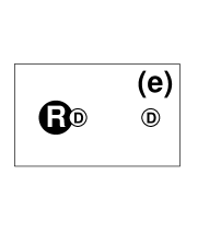
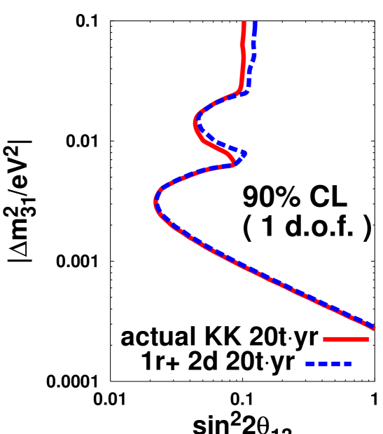
To see how effectively the correlated errors are canceled in the actual KASKA plan, comparison is given in Fig.2 between the sensitivities to $\sin^{2}2\theta$ of the actual KASKA plan (Fig.1(c)) and of a hypothetical experiment with a single reactor and two detectors (300m and 1.3km baselines) depicted in Fig.1(e)); The same value of uncorrelated systematic error $\sigma_{u}$ and the same data size (=20t$\cdot$yr) are used for each case. We observe that there is little difference between the sensitivities at $\Delta m^{2}=2.5\times 10^{-3}\text{eV}^{2}$. Also it is remarkable that the sensitivity of the actual KASKA plan for higher value of $\Delta m^{2}$ is better than of the single reactor experiment. This is exactly because of the reduction of the uncorrelated error from due to the nature of multi reactors (cf. Eq. (22)), where the near detectors play a role as far detectors in this case. Here, it should be mentioned that we see in Fig. 2 that the sensitivity in KASKA changes only to $\sin^{2}{2\theta}\simeq 0.03$ even for $\Delta m^{2}=2\times 10^{-3}\text{eV}^{2}$.

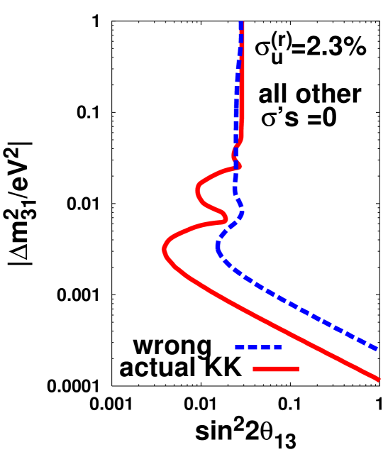
Now let us see the effects of multiple sources on the systematic limit $\left(\sin^{2}2\theta\right)_{\text{limit}}^{\text{sys~{}only}}$ in the KASKA plan. Since the effect comes with $\sigma_{\text{u}}^{(\text{r})}$ (compare (20) with (3)), we can ignore other errors. The systematic limit for the case is presented in Fig. 3 with solid line; $\sigma_{\text{u}}^{(\text{r})}$ is assumed to be 2.3%. Note that the systematic limit is extremely close to zero for one reactor case because of ideal near-far cancellation. The solid line in Fig. 3 shows, however, that about 0.4% error remains. Thus, we find that the effect of the nature of multiple sources is only about 0.4%. It is vary small compared to the relative normalization error $\sqrt{2}\sigma_{\text{u}}(\simeq 0.8\%)$ of the detectors. Once we know that two near detectors are sufficient for near-far cancellation with the Kashiwazaki-Kariwa nuclear power station, we should investigate the optimal locations of the near detectors for the cancellation. While the two near detectors are assumed to be very close to the reactors in the ideal limit (Fig. 1(d)), the near detectors in the actual KASKA case cannot be too close to the reactors. If each of the two near detectors is too close to a reactor, it is impossible to cancel the uncorrelated error of the flux from other reactors, namely $\sigma_{\text{u}}^{\text{(}r)}$. Hence, the optimization of the locations of two near detectors at the Kashiwazaki-Kariwa site is nontrivial. At first, in order to see the importance of the location of near detectors, we compare the systematic limits of the actual KASKA plan (Fig. 1(c)) with that of a hypothetical experiment (Fig. 1(f)) in Fig. 3; In the hypothetical experiment, one near detector is very close to the reactor #1 in the first cluster while the other detector is very close to the reactor #5 in the second one. In Fig. 3 we use $\sigma_{\text{u}}^{\text{(r)}}=2.3\%$ and all other systematic errors are set to zero because $\sigma_{\text{u}}^{\text{(r)}}$ dominates the difference of near-far cancellations in the two cases. For $\Delta m^{2}=2.5\times 10^{-3}\text{eV}^{2}$, we obtain $\left(\sin^{2}2\theta\right)_{\text{limit}}^{\text{sys~{}only}}\simeq 4\times 10^{-3}~{}(2\times 10^{-2})$ for the actual KASKA plan (the hypothetical case). In the hypothetical case, the sensitivity is deteriorated because the correlated error $\sigma_{\text{u}}^{\text{(r)}}$ is not canceled sufficiently and about 2% error remains.

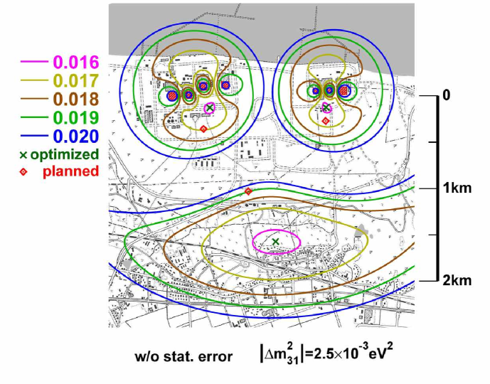
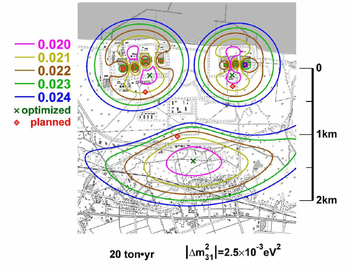
We can extend this analysis to that with the arbitrary position of each detector. To do the analysis, we first obtain the optimized positions of the detectors. And then we examine the sensitivity to $\sin^{2}2\theta$ by varying the position of each detector, leaving the locations of the remaining detectors in the optimized ones. The results are given by the contour plots in Fig. 4 without statistical errors and in Fig. 5 with the data size of 20 ton$\cdot$yr, where the reference values in Eqs. (1) and (2) are used. In these figures the locations of the detectors are also depicted for the optimized case and for the currently planned case. From these two figures we observe that the distance between each near detector and the reactors in each cluster is approximately (300$\pm$130)m in the optimized case. This results in slightly poorer sensitivity to $\sin^{2}2\theta$, compared with the hypothetical single reactor case with a near detector which is arbitrarily close to the reactor (See Eq. (19) with $L_{\text{n}}=0$). From Figs. 3, 4, 5, we see that the positions of the near detectors in the KASKA plan are appropriate for the near-far cancellation and almost optimized. Therefore, it does not suffer from the multi-reactor nature such as the variety of reactor powers or distances between the reactors and the near detectors.

V Discussion and Conclusion

Using the analytical method, we estimated the systematic limits (sensitivity without statistical error) on the neutrino oscillation parameter $\sin^{2}2\theta_{13}$ in various setups of reactor experiments. In the simplest case, where there is one reactor and two detectors, the correlated systematic error is canceled. In the case of multiple $n_{r}$ reactors, we showed that the correlated systematic errors of the reactors and the detectors are canceled as naive expectation if the number of detectors $n_{d}$ is sufficient ($n_{d}=n_{r}+1$). We found that multiple reactors and detectors set up has an advantage of the reduction of the remaining uncorrelated error if the set up is appropriate for the near-far cancellation of correlated errors. On the other hand, we explicitly showed that the contribution to the sensitivity to $\sin^{2}2\theta_{13}$ from the the uncorrelated error of the flux, which controls the multi-reactor nature, is negligibly small although there are only three detectors for seven reactors ($n_{d}<n_{r}+1$). The only disadvantage of experiments with $n_{d}<n_{r}+1$ is that one cannot put the near detectors arbitrarily close to one of the reactors (even if one neglects the technical difficulties), because that would ruin the cancellation of the uncorrelated error of the flux, as we have seen explicitly in the KASKA case. We presented also the optimal positions of detectors in the KASKA plan; The planned position of near detectors are close to the optimal ones although it is better if the baseline length for the far detector becomes longer beyond the bound of the power station site. In all cases studies here, it is the factor $\sigma_{\text{u}}/\left[\left\langle\sin^{2}\left(\Delta m^{2}L_{\text{f}}/4E\right)\right\rangle-\left\langle\sin^{2}\left(\Delta m^{2}L_{\text{n}}/4E\right)\right\rangle\right]$ that sets the systematic limit on $\sin^{2}2\theta_{13}$, and hence it is quite important to estimate $\sigma_{\text{u}}$ carefully. The factor $\left(\sin^{2}2\theta\right)_{\text{limit}}^{\text{sys~{}only}}/\sigma_{\text{u}}$ seems to be a good measure of the power of a reactor experiment almost independently of assumptions of error sizes.

Appendix A Derivation of the covariance matrix

In this appendix we first show that the form of $\chi^{2}$ which is expressed as the minimum of the function of the $\alpha$ variables with respect to these variables leads to the form of $\chi^{2}$ which is bilinear in the ratio $m_{j}/t_{j}$ of the measured value $m_{j}$ divided by the theoretical prediction $t_{j}$. This has been known in the literature Stump:2001gu ; Botje:2001fx ; Pumplin:2002vw ; Fogli:2002pt as the equivalence between the so-called pull approach and the covariance matrix approach. And then we show that the same job can be done by integration of $\exp(-\chi^{2}/2)$ over the variables $m_{j}/t_{j}$.

In the cases which we are considering, the correlated systematic errors $t_{1}^{2}\sigma_{\text{u}\,1}^{2},\cdots,t_{n}^{2}\sigma_{\text{u}\,\ell}^{2}$ are introduced by the variables

$$\vec{\alpha}\equiv\left(\begin{array}[]{cc}\alpha_{1}\\ \vdots\\ \alpha_{\ell}\end{array}\right).$$ (82)

Introducing the notation

$$y_{j} \equiv \displaystyle{m_{j}\over t_{j}}-1,$$

$$\vec{y} \equiv \left(\begin{array}[]{cc}y_{1}\\ \vdots\\ y_{n}\end{array}\right),$$ (86)

$\chi^{2}$ can be written as

$$\chi^{2} = \min_{\vec{\alpha}}\left[\left(\vec{y}-H\vec{\alpha}\right)^{T}D_{\text{u}}^{-1}\left(\vec{y}-H\vec{\alpha}\right)+\vec{\alpha}^{T}D_{\text{c}}^{-1}\vec{\alpha}\right]$$ (87)

$$= \min_{\vec{\alpha}}\left[\left(\vec{\alpha}-A^{-1}HD_{\text{u}}^{-1}\vec{y}\right)^{T}A\left(\vec{\alpha}-A^{-1}HD_{\text{u}}^{-1}\vec{y}\right)+\vec{y}^{T}\left(D_{\text{u}}^{-1}-D_{\text{u}}^{-1}HA^{-1}H^{T}D_{\text{u}}^{-1}\right)\vec{y}\right]$$

$$= \vec{y}^{\,T}\left(D_{\text{u}}^{-1}-D_{\text{u}}^{-1}HA^{-1}H^{T}D_{\text{u}}^{-1}\right)\vec{y},$$

where

$$H \equiv \left(\begin{array}[]{ccc}1&\cdots\cdots&1\\ \vdots&&\vdots\\ 1&\cdots\cdots&1\end{array}\right),$$ (91)

is an $n\times\ell$ matrix,

$$D_{\text{u}} \equiv \mbox{\rm diag}\left(\sigma_{\text{u}\,1}^{2},\cdots,\sigma_{\text{u}\,n}^{2}\right)$$

is an $n\times n$ diagonal matrix whose element is the normalized uncorrelated systematic error $\sigma_{\text{u}\,j}^{2}$ for the variable $m_{j}$ ($j=1,\cdots,n$),

$$D_{\text{c}} \equiv \mbox{\rm diag}\left(\sigma_{\text{c}\,1}^{2},\cdots,\sigma_{\text{c}\,\ell}^{2}\right)$$

is an $\ell\times\ell$ diagonal matrix whose element is the normalized correlated systematic error $\sigma_{\text{c}\,j}^{2}$ for the variable $\alpha_{j}$ ($j=1,\cdots,\ell$), and we have defined

$$A\equiv D_{\text{c}}^{-1}+H^{T}D_{\text{u}}^{-1}H.$$

Note that we can incorporate the effect of the statistical errors in our formalism by redefining $D_{u}\rightarrow\mbox{\rm diag}(\sigma_{\text{u}\,1}^{2}+1/\sqrt{t_{1}},\cdots,\sigma_{\text{u}\,1}^{2}+1/\sqrt{t_{n}})$, although we do not discuss the statistical errors in the present paper. From Eq. (87) we see that the covariance matrix $V$ is given by

$$V=\left(D_{\text{u}}^{-1}-D_{\text{u}}^{-1}HA^{-1}H^{T}D_{\text{u}}^{-1}\right)^{-1}.$$

We could prove by brute force that $V$ can be written as

$$V=D_{\text{u}}+HD_{\text{c}}H^{T},$$ (92)

but it is much easier to prove it by expressing the matrix element $V_{ij}$ as the integral of $\exp(-\chi^{2}/2)$ over the variables $y_{j}$.

First of all, let us prove that the matrix element $V_{ij}$ can be written as

$$V_{ij}={\cal N}_{y}\int d\vec{y}\,y_{i}y_{j}\,\exp\left(-{1\over 2}\vec{y}^{\,T}V^{-1}\vec{y}\right),$$ (93)

where ${\cal N}_{y}$ is the normalization constant defined by

$${\cal N}_{y}^{-1}\equiv\int d\vec{y}\,\exp\left(-{1\over 2}\vec{y}^{\,T}V^{-1}\vec{y}\right).$$

Proof of Eq. (93) goes as follows. Diagonalizing the covariance matrix $V$, which is real symmetric, by an orthogonal matrix ${\cal O}$

$$V={\cal O}^{T}D{\cal O}\equiv{\cal O}^{T}\mbox{\rm diag}\left(v_{1},\cdots,v_{n}\right){\cal O},$$

the exponent can be rewritten as

$$\vec{y}^{\,T}V^{-1}\vec{y}=\vec{y}^{\,T}{\cal O}^{T}D^{-1}{\cal O}\vec{y}\equiv\vec{y^{\prime}}^{\,T}D^{-1}\vec{y^{\prime}},$$

so that we have

$${\cal N}_{y}\int d\vec{y}\,y_{i}y_{j}\,\exp\left(-{1\over 2}\vec{y}^{\,T}V^{-1}\vec{y}\right)$$

$$= {\cal N}_{y}\int d\vec{y^{\prime}}\,\left({\cal O}^{T}\vec{y^{\prime}}\right)_{i}\left({\cal O}^{T}\vec{y^{\prime}}\right)_{j}\,\exp\left(-{1\over 2}\vec{y^{\prime}}^{\,T}D^{-1}\vec{y^{\prime}}\right)$$

$$= {\cal N}_{y}\int d\vec{y^{\prime}}\,\left({\cal O}\right)_{ki}y^{\prime}_{k}\left({\cal O}\right)_{lj}y^{\prime}_{l}\,\exp\left(-{1\over 2}\sum_{i=1}^{n}\displaystyle{y_{j}^{{}^{\prime}2}\over v_{j}}\right)$$

$$= \left({\cal O}\right)_{ki}\left(D\right)_{kl}\left({\cal O}\right)_{lj}$$

$$= \left({\cal O}^{T}D{\cal O}\right)_{ij}$$

$$= V_{ij}.$$

Thus Eq. (93) is proved.

Now Eq. (93) can be simplified by expressing as the integral over the variables $\vec{\alpha}$ of the original $\chi^{2}$:

$$V_{ij} = {\cal N}_{y}\int d\vec{y}\,y_{i}y_{j}\,\exp\left(-{1\over 2}\vec{y}^{\,T}V^{-1}\vec{y}\right)$$ (94)

$$= {\cal N}_{y}{\cal N}_{\alpha}\int d\vec{y}\,\int d\vec{\alpha}\,y_{i}y_{j}\,\exp\left\{-{1\over 2}\left[\left(\vec{\alpha}-A^{-1}HD_{\text{u}}^{-1}\vec{y}\right)^{T}A\left(\vec{\alpha}-A^{-1}HD_{\text{u}}^{-1}\vec{y}\right)\right.\right.$$

$$\left.\left.+\vec{y}^{T}\left(D_{\text{u}}^{-1}-D_{\text{u}}^{-1}HA^{-1}H^{T}D_{\text{u}}^{-1}\right)\vec{y}\right]\right\}$$

$$= {\cal N}_{y}{\cal N}_{\alpha}\int d\vec{y}\,\int d\vec{\alpha}\,y_{i}y_{j}\,\exp\left\{-{1\over 2}\left[\left(\vec{y}-H\vec{\alpha}\right)^{T}D_{\text{u}}^{-1}\left(\vec{y}-H\vec{\alpha}\right)+\vec{\alpha}^{T}D_{\text{c}}^{-1}\vec{\alpha}\right]\right\},$$

where we have used Eq. (87), the normalization constant ${\cal N}_{\alpha}$ is defined by

$${\cal N}_{\alpha}^{-1} \equiv \int d\vec{\alpha}\,\exp\left\{-{1\over 2}\left[\left(\vec{\alpha}-A^{-1}HD_{\text{u}}^{-1}\vec{y}\right)^{T}A\left(\vec{\alpha}-A^{-1}HD_{\text{u}}^{-1}\vec{y}\right)\right]\right\},$$

and ${\cal N}_{y}$ and ${\cal N}_{\alpha}$ are related by

$${\cal N}_{y}{\cal N}_{\alpha}=\left(2\pi\right)^{(n+\ell)/2}\left(\det D_{\text{u}}\right)^{1/2}\left(\det D_{\text{c}}\right)^{1/2}.$$

Eq. (94) can be easily calculated by shifting the variable $\vec{y}\rightarrow\vec{y^{\prime\prime}}\equiv\vec{y}-H\vec{\alpha}$:

$$V_{ij} = {\cal N}_{y}{\cal N}_{\alpha}\int d\vec{y^{\prime\prime}}\,\int d\vec{\alpha}\,\left(\vec{y^{\prime\prime}}-H\vec{\alpha}\right)_{i}\left(\vec{y^{\prime\prime}}-H\vec{\alpha}\right)_{j}$$

$$\exp\left\{-{1\over 2}\left[\left(\vec{y}-H\vec{\alpha}\right)^{T}D_{\text{u}}^{-1}\left(\vec{y}-H\vec{\alpha}\right)+\vec{\alpha}^{T}D_{\text{c}}^{-1}\vec{\alpha}\right]\right\}$$

$$= \left(D_{\text{u}}\right)_{ij}+\left(H\right)_{ik}\left(H\right)_{jl}\left(D_{\text{c}}\right)_{kl}$$

$$= \left(D_{\text{u}}+HD_{\text{c}}H^{T}\right)_{ij}.$$

Hence Eq. (92) is proved.

In the case of one reactor with one detector (cf. Eq. (3)), we have

$$D_{\text{u}} = \sigma_{\text{u}}^{2}$$

$$D_{\text{c}} = {\rm diag}\left(\sigma_{\text{c}}^{2},(\sigma_{\text{c}}^{\text{(r)}})^{2},(\sigma_{\text{u}}^{\text{(r)}})^{2}\right)$$

$$H = (1,1,1),$$

so the covariance matrix is

$$V=D_{\text{u}}+HD_{\text{c}}H^{T}=\sigma_{\text{u}}^{2}+\sigma_{\text{c}}^{2}+(\sigma_{\text{c}}^{\text{(r)}})^{2}+(\sigma_{\text{u}}^{\text{(r)}})^{2}.$$

In the case of one reactor with two detectors (cf. Eq. (13)), we have

$$D_{\text{u}} = \sigma_{\text{u}}^{2}\,\left(\begin{array}[]{cc}1&0\\ 0&1\\ \end{array}\right)$$ (97)

$$D_{\text{c}} = {\rm diag}\left(\sigma_{\text{c}}^{2},(\sigma_{\text{c}}^{\text{(r)}})^{2},(\sigma_{\text{u}}^{\text{(r)}})^{2}\right)$$

$$H = \left(\begin{array}[]{ccc}1&1&1\\ 1&1&1\\ \end{array}\right),$$ (100)

so that we obtain

$$V=D_{\text{u}}+HD_{\text{c}}H^{T}=\left(\displaystyle\begin{array}[]{rr}\sigma^{2}_{\text{u}}+\sigma^{2}_{\text{c}}+(\sigma^{\text{(r)}}_{\text{u}})^{2}+(\sigma^{\text{(r)}}_{\text{c}})^{2}&\quad\sigma^{2}_{\text{c}}+(\sigma^{\text{(r)}}_{\text{u}})^{2}+(\sigma^{\text{(r)}}_{\text{c}})^{2}\\ \quad\sigma^{2}_{\text{c}}+(\sigma^{\text{(r)}}_{\text{u}})^{2}+(\sigma^{\text{(r)}}_{\text{c}})^{2}&\sigma^{2}_{\text{u}}+\sigma^{2}_{\text{c}}+(\sigma^{\text{(r)}}_{\text{u}})^{2}+(\sigma^{\text{(r)}}_{\text{c}})^{2}\end{array}\right).$$ (103)

In the case of $n_{r}$ reactors with one detector (cf. Eq. (20)), we have

$$D_{\text{u}} = \sigma_{\text{u}}^{2}$$

$$D_{\text{c}} = {\rm diag}\left[\sigma_{\text{c}}^{2},(\sigma_{\text{c}}^{\text{(r)}})^{2},(\sigma_{\text{u}}^{\text{(r)}})^{2},\cdots,(\sigma_{\text{u}}^{\text{(r)}})^{2}\right]$$

$$H = \left(1,1,{t_{1}\over t},\cdots,{t_{n_{r}}\over t}\right),$$

so that we obtain

$$V = D_{\text{u}}+HD_{\text{c}}H^{T}$$

$$= \sigma_{\text{u}}^{2}+\left(1,1,{t_{1}\over t},\cdots,{t_{n_{r}}\over t}\right){\rm diag}\left[\sigma_{\text{c}}^{2},(\sigma_{\text{c}}^{\text{(r)}})^{2},(\sigma_{\text{u}}^{\text{(r)}})^{2},\cdots,(\sigma_{\text{u}}^{\text{(r)}})^{2}\right]\left(\begin{array}[]{c}1\\ 1\\ {t_{1}/t}\\ \vdots\\ {t_{n_{r}}/t}\end{array}\right)$$

$$= \sigma_{\text{u}}^{2}+\sigma_{\text{c}}^{2}+(\sigma_{\text{c}}^{\text{(r)}})^{2}+(\sigma_{\text{u}}^{\text{(r)}})^{2}\sum_{a=1}^{n_{r}}\left({t_{a}\over t}\right)^{2}.$$

In the case of $n_{r}$ reactors with $n_{d}$ detector (cf. Eq. (27)), we have

$$D_{\text{u}} = \sigma_{\text{u}}^{2}\,I_{n_{d}}$$

$$D_{\text{c}} = {\rm diag}\left[\sigma_{\text{c}}^{2},(\sigma_{\text{c}}^{\text{(r)}})^{2},(\sigma_{\text{u}}^{\text{(r)}})^{2},\cdots,(\sigma_{\text{u}}^{\text{(r)}})^{2}\right]$$

$$H = \left(\begin{array}[]{ccccc}1&1&{t_{1}\over t}&\cdots&{t_{n_{r}}\over t}\\ \vdots&\vdots&\vdots&\vdots&\vdots\\ 1&1&{t_{1}\over t}&\cdots&{t_{n_{r}}\over t}\\ \end{array}\right),$$ (113)

where $I_{n_{d}}$ is an $n_{d}\times n_{d}$ unit matrix, so that we obtain

$$V = \sigma_{\text{u}}^{2}I_{n_{d}}+\left(\begin{array}[]{ccccc}1&1&{t_{1}\over t}&\cdots&{t_{n_{r}}\over t}\\ \vdots&\vdots&\vdots&\vdots&\vdots\\ 1&1&{t_{1}\over t}&\cdots&{t_{n_{r}}\over t}\\ \end{array}\right){\rm diag}\left[\sigma_{\text{c}}^{2},(\sigma_{\text{c}}^{\text{(r)}})^{2},(\sigma_{\text{u}}^{\text{(r)}})^{2},\cdots,(\sigma_{\text{u}}^{\text{(r)}})^{2}\right]\left(\begin{array}[]{ccc}1&\cdots&1\\ 1&\cdots&1\\ {t_{1}/t}&\cdots&{t_{1}/t}\\ \vdots&\vdots&\vdots\\ {t_{n_{r}}/t}&\cdots&{t_{n_{r}}/t}\end{array}\right)$$

$$= \sigma_{\text{u}}^{2}I_{n_{d}}+\left[\sigma_{\text{c}}^{2}+(\sigma_{\text{c}}^{\text{(r)}})^{2}+(\sigma_{\text{u}}^{\text{(r)}})^{2}\sum_{a=1}^{n_{r}}\left({t_{a}\over t}\right)^{2}\right]H_{n_{d}},$$

where $H_{n_{d}}$ is an $n_{d}\times n_{d}$ matrix whose elements are all 1 (cf. Eq. (38)).

Appendix B Derivation of $\chi^{2}$ (53) in the case with $n_{r}$ reactors and $n_{r}+1$ detectors

$V$ in Eq. (34) can be diagonalized as

$$U^{-1}VU$$

$$= \mbox{\rm diag}\left\{(n_{r}+1)\left[\sigma_{\text{c}}^{2}+\left(\sigma_{\text{c}}^{(r)}\right)^{2}+{\sigma_{\text{u}}^{2}\over n_{r}}+{\left(\sigma_{\text{u}}^{(r)}\right)^{2}\over n_{r}}\right],\sigma_{\text{u}}^{2}+\left(\sigma_{\text{u}}^{(r)}\right)^{2},\cdots,\sigma_{\text{u}}^{2}+\left(\sigma_{\text{u}}^{(r)}\right)^{2},\sigma_{\text{u}}^{2}\right\},$$

where $U$ is a unitary matrix defined by

$$U = \left(\vec{u}^{(1)},\cdots,\vec{u}^{(n)}\right),$$

$$\vec{u}^{(1)} \equiv {1\over\sqrt{N_{r}+1}}\left(\begin{array}[]{c}1\\ \vdots\\ 1\end{array}\right),\quad\vec{u}^{(2)}\equiv{1\over\sqrt{2}}\left(\begin{array}[]{r}1\\ -1\\ 0\\ \vdots\\ 0\end{array}\right),$$ (131)

$$\vec{u}^{(3)} \equiv {1\over\sqrt{6}}\left(\begin{array}[]{r}1\\ 1\\ -2\\ 0\\ \vdots\\ 0\end{array}\right),\cdots,\quad\vec{u}^{(n_{r}+1)}\equiv{1\over\sqrt{n_{r}(n_{r}+1)}}\left(\begin{array}[]{r}1}{\\ \vdots{}}{\\ 1}{\\ -n_{r}\end{array}\right).$$ (142)

Introducing the notation

$$\vec{y}\equiv\left(\begin{array}[]{c}m_{1}/t_{1}-1\\ \vdots\\ m_{n_{r}}/t_{n_{r}}-1\\ m_{n_{r}+1}/t_{n_{r}+1}-1\\ \end{array}\right),$$ (147)

$\chi^{2}$ can be written as

$$\chi^{2} = {\left(\vec{y}\cdot\vec{u}^{(1)}\right)^{2}\over\sigma_{\text{u}}^{2}+(n_{r}+1)\left[\sigma_{\text{c}}^{2}+\left(\sigma_{\text{c}}^{(r)}\right)^{2}+\left(\sigma_{\text{u}}^{(r)}\right)^{2}/n_{r}\right]}+{\displaystyle\sum_{j=2}^{n_{r}}\left(\vec{y}\cdot\vec{u}^{(j)}\right)^{2}\over\sigma_{\text{u}}^{2}+\left(\sigma_{\text{u}}^{(r)}\right)^{2}}+{\left(\vec{y}\cdot\vec{u}^{(n_{r}+1)}\right)^{2}\over\sigma_{\text{u}}^{2}}.$$

From Eq. (142) we have $\vec{y}\cdot\vec{u}_{1}=D(L_{\text{f}})/\sqrt{n_{r}+1}$, $\vec{y}\cdot\vec{u}_{j}=0~{}(j=2,\cdots,n_{r})$, $\vec{y}\cdot\vec{u}_{n_{r}+1}=-\sqrt{n_{r}/(n_{r}+1)}D(L_{\text{f}})$, and we finally get

$$\chi^{2} = \left[D(L_{\text{f}})\right]^{2}\left\{{n_{r}\over n_{r}+1}{1\over\sigma_{\text{u}}^{2}}+{1\over n_{r}+1}{1\over\sigma_{\text{u}}^{2}+(n_{r}+1)\left[\sigma_{\text{c}}^{2}+\left(\sigma_{\text{c}}^{(r)}\right)^{2}+\left(\sigma_{\text{u}}^{(r)}\right)^{2}/n_{r}\right]}\right\}.$$

Appendix C Derivation of the systematic limit in the KASKA plan

It is easy to show that the diagonalized matrix out of the covariance matrix $V$ (LABEL:v7r3d) is

$$\mbox{\rm diag}(\sigma_{\text{u}}^{2},\sigma_{\text{u}}^{2}+\Lambda_{+},\sigma_{\text{u}}^{2}+\Lambda_{-}),$$ (148)

where

$$\Lambda_{\pm} \equiv {3\over 2}\left[\sigma_{\text{c}}^{2}+(\sigma^{\text{(r)}}_{\text{c}})^{2}\right]+{61\over 168}(\sigma^{\text{(r)}}_{\text{u}})^{2}$$

$$\pm \displaystyle{1\over 2}\left\{9\left[\sigma_{\text{c}}^{2}+(\sigma^{\text{(r)}}_{\text{c}})^{2}\right]^{2}+{5\over 6}\left[\sigma_{\text{c}}^{2}+(\sigma^{\text{(r)}}_{\text{c}})^{2}\right](\sigma^{\text{(r)}}_{\text{u}})^{2}+\left({13\over 84}\right)^{2}(\sigma^{\text{(r)}}_{\text{u}})^{4}\right\}^{1/2}.$$

The corresponding eigenvectors are

$$\vec{u}^{(1)}={1\over\sqrt{74}}\left(\begin{array}[]{c}-4\\ -3\\ 7\\ \end{array}\right),\vec{u}^{(2)}={\cal N}_{+}\left(\begin{array}[]{c}-\Lambda_{+}+46\eta\\ -\Lambda_{+}+53\eta\\ -\Lambda_{+}+49\eta\end{array}\right),\vec{u}^{(3)}={\cal N}_{-}\left(\begin{array}[]{c}-\Lambda_{-}+46\eta\\ -\Lambda_{-}+53\eta\\ -\Lambda_{-}+49\eta\end{array}\right),$$ (158)

where

$$\eta\equiv{1\over 84}\,{(\sigma_{\text{u}}^{\text{(r)}})^{2}\over\sigma_{\text{c}}^{2}+(\sigma_{\text{c}}^{\text{(r)}})^{2}},$$

and ${\cal N}_{\pm}$ are the normalization constants. Hence we get

$$\chi^{2} = \sin^{4}2\theta\left\{\displaystyle{49\over 74}\displaystyle{\left[D(L_{\text{f}})\right]^{2}\over\sigma_{\text{u}}^{2}}+\displaystyle{\left[u_{3}^{(2)}D(L_{\text{f}})\right]^{2}\over\sigma_{\text{u}}^{2}+\Lambda_{-}}+\displaystyle{\left[u_{3}^{(3)}D(L_{\text{f}})\right]^{2}\over\sigma_{\text{u}}^{2}+\Lambda_{+}}\right\}$$

$$\simeq \sin^{4}2\theta\,\displaystyle{49\over 74}\,\displaystyle{\left[D(L_{\text{f}})\right]^{2}\over\sigma_{\text{u}}^{2}}.$$

In the actual KASKA case, using the reference values (1) and (2), from numerical calculations we obtain the diagonalized covariance matrix

$$\mbox{\rm diag}(\lambda_{1},\lambda_{2},\lambda_{3})=\sigma_{\text{u}}^{2}\mbox{\rm diag}(1.044,4.651,90.878),$$

and the corresponding three eigenvectors

$$\vec{u}^{(1)}\equiv\left(\begin{array}[]{c}u_{1}^{(1)}\\ u_{2}^{(1)}\\ u_{3}^{(1)}\\ \end{array}\right)=\left(\begin{array}[]{c}-0.4975\\ -0.3114\\ 0.8097\\ \end{array}\right),~{}\vec{u}^{(2)}=\left(\begin{array}[]{c}0.6503\\ -0.7516\\ 0.1105\\ \end{array}\right),~{}\vec{u}^{(3)}=\left(\begin{array}[]{c}0.5741\\ 0.5815\\ 0.5764\\ \end{array}\right).$$ (171)

$\chi^{2}$ can be written as

$$\chi^{2}={\left(\vec{y}\cdot\vec{u}^{(1)}\right)^{2}\over\lambda_{1}}+{\left(\vec{y}\cdot\vec{u}^{(2)}\right)^{2}\over\lambda_{2}}+{\left(\vec{y}\cdot\vec{u}^{(3)}\right)^{2}\over\lambda_{3}}\simeq{\left(\vec{y}\cdot\vec{u}^{(1)}\right)^{2}\over\lambda_{1}},$$

where $\vec{y}$ in this case is given by

$$\vec{y}\equiv\left(\begin{array}[]{c}{m_{1}\over t_{1}}-1\\ {m_{2}\over t_{2}}-1\\ {m_{3}\over t_{3}}-1\\ \end{array}\right)=-\sin^{2}2\theta\left(\begin{array}[]{c}\displaystyle\sum_{a=1}^{7}{t_{a1}\over t_{1}}D(L_{a1})\\ \displaystyle\sum_{a=1}^{7}{t_{a2}\over t_{2}}D(L_{a2})\\ \displaystyle\sum_{a=1}^{7}{t_{a3}\over t_{3}}D(L_{a3})\\ \end{array}\right)\equiv-\sin^{2}2\theta\left(\begin{array}[]{c}\overline{D(L_{1})}\\ \overline{D(L_{2})}\\ \overline{D(L_{3})}\\ \end{array}\right)$$ (181)

using the definition of $D(L)$ in Eq. (16) and $\overline{D(L_{j})}$ in Eq. (78). Hence we get

$$\chi^{2}\simeq{\sin^{4}2\theta\over 1.04\sigma_{\text{u}}^{2}}\left[\overline{D(L_{3})}u^{(1)}_{3}+\overline{D(L_{1})}u^{(1)}_{1}+\overline{D(L_{2})}u^{(1)}_{2}\right]^{2},$$

from which Eq. (77) follows.

Reactors($a$)	Power/GWth	$L_{a\,1}$/m	$L_{a\,2}$/m	$L_{a\,3}$/m
1	3.293	482	1663	1309
2	3.293	401	1504	1224
3	3.293	458	1374	1233
4	3.293	524	1149	1169
5	3.293	1552	371	1484
6	3.926	1419	333	1397
7	3.926	1280	340	1306

Table 1: The Power of the the reactors in GW${}_{\text{th}}$ and the distance $L_{aj}$ in meters from the three detectors ($j$=1(near), 2(near), 3(far)) to each reactor ($a=1,\cdots,7$). The powers of reactors are listed in http://www.tepco.co.jp/kk-np/index-j.html. The positions of the reactors were read from a map and are subject to a few meters of inaccuracy. However, such inaccuracy hardly affects the estimation of the systematic errors in the text.

Reactors($a$)	$t_{a1}/t_{1}$	$t_{a2}/t_{2}$	$t_{a3}/t_{3}$
1	0.208	0.012	0.133
2	0.301	0.015	0.152
3	0.231	0.017	0.149
4	0.176	0.025	0.166
5	0.020	0.239	0.103
6	0.029	0.353	0.139
7	0.035	0.339	0.159

Table 2: The fraction $t_{aj}/t_{j}$ of the yields at each detector $j$ from the reactor $a$ in the KASKA plan.

Figure 1: Configurations of the experiments: (a) $n_{r}$ reactors + one detector. (b) $n_{r}$ reactors + $(n_{r}+1)$ detectors. (c) The KASKA plan with 7 reactors + 3 detectors. (d) The ideal limit of the KASKA plan. (e) One reactor + 2 detectors to be compared with (c). (f) The hypothetical KASKA plan with the near detectors in the wrong locations to be compared with (c).

Figure 2: The comparison of the sensitivity to $\sin^{2}2\theta_{13}$ for the actual KASKA plan (the solid line; with the configuration depicted in Fig.1(c)) and a hypothetical case (the dashed line; with the configuration depicted in Fig.1(e)). The statistical errors as well as all the systematic errors are taken into account.

Figure 3: The comparison of the locations of the near detectors in the KASKA plan. The solid (dashed) line is for the actual (hypothetical) KASKA plan with the location depicted in Fig.1(c) (Fig.1(f)), respectively.

Figure 4: The contour plots of the systematic limit on $\sin^{2}2\theta_{13}$ in the KASKA experiment. The optimized and currently planned positions of the detectors are also depicted. When the contour for each detector is plotted, it is assumed that other detectors are located in the optimized positions.

Figure 5: The same contour plot of the sensitivity to $\sin^{2}2\theta_{13}$ as Fig. 4 with the data size of 20ton$\cdot$yr.

References

• (1) Y. Kozlov, L. Mikaelyan and V. Sinev, Phys. Atom. Nucl.  66, 469 (2003) [Yad. Fiz.  66, 497 (2003)] [arXiv:hep-ph/0109277]; V. Martemyanov, L. Mikaelyan, V. Sinev, V. Kopeikin and Y. Kozlov, arXiv:hep-ex/0211070.
• (2) H. Minakata, H. Sugiyama, O. Yasuda, K. Inoue and F. Suekane, Phys. Rev. D 68, 033017 (2003) [arXiv:hep-ph/0211111].
• (3) P. Huber, M. Lindner, T. Schwetz and W. Winter, Nucl. Phys. B 665, 487 (2003) [arXiv:hep-ph/0303232].
• (4) M. Kuze, talk at “6th International Workshop on Neutrino Factories and Superbeams (NuFact04)“, Jul.26-Aug.1, 2004, Osaka, Japan.
• (5) arXiv:hep-ex/0405032.
• (6) M. H. Shaevitz and J. M. Link, arXiv:hep-ex/0306031.
• (7) T. Bolton, talk at “6th International Workshop on Neutrino Factories and Superbeams (NuFact04)“, Jul.26-Aug.1, 2004, Osaka, Japan.
• (8) Y. Wang, talk at “3rd Workshop on Future Low-Energy Neutrino Experiments”, Mar. 20-22, 2004, Niigata, Japan.
• (9) K. Anderson et al., arXiv:hep-ex/0402041.
• (10) D. Stump et al., Phys. Rev. D 65, 014012 (2002) [arXiv:hep-ph/0101051].
• (11) M. Botje, J. Phys. G 28, 779 (2002) [arXiv:hep-ph/0110123].
• (12) J. Pumplin, D. R. Stump, J. Huston, H. L. Lai, P. Nadolsky and W. K. Tung, JHEP 0207, 012 (2002) [arXiv:hep-ph/0201195].
• (13) G. L. Fogli, E. Lisi, A. Marrone, D. Montanino and A. Palazzo, Phys. Rev. D 66, 053010 (2002) [arXiv:hep-ph/0206162].
• (14) Y. Declais et al., Nucl. Phys. B 434, 503 (1995).
• (15) K. Eguchi et al. [KamLAND Collaboration], Phys. Rev. Lett.  90, 021802 (2003) [arXiv:hep-ex/0212021].