Simulating $W$/$Z$+jets production at the Tevatron

Abstract

The merging procedure of tree-level matrix elements and the subsequent parton shower as implemented in the new event generator SHERPA will be validated for the example of $W$/$Z$+jets production at the Tevatron. Comparisons with results obtained from other approaches and programs and with experimental results clearly show that the merging procedure yields relevant and correct results at both the hadron and parton levels.

I Introduction

The production of electroweak gauge bosons, e.g. $W^{\pm}$ and $Z$ bosons, is one of the most prominent processes at hadron colliders. Especially through their leptonic decays they leave a clean signature, namely either one charged lepton accompanied by missing energy for $W$ bosons or two oppositely charged leptons for the $Z$ bosons. The combination of clear signatures and copious production rates allows a measurement of some of their parameters, e.g. the $W$ mass and width, with a precision comparable with that reached at LEP2 at the Tevatron Abachi:1995xc ; Affolder:2000bp ; Abazov:2002bu ; unknown:2003sv ; Albajar:1990hg ; Alitti:1991dm ; Abe:1995wf ; Abbott:1999tt ; Affolder:2000mt ; Abazov:2002xj , or even better at the LHC ATLAS_TDR ; Haywood:1999qg . The same combination, clear signature and large production rate, renders them a good candidate process for luminosity measurements, especially at the LHC Khoze:2000db ; Dittmar:1997md ; Martin:1999ww ; Giele:2001ms . This holds true in particular for $W$-bosons, since their production rate is enhanced by roughly an order of magnitude with respect to $Z$ production. Furthermore, especially in combination with additional jets, the production of gauge bosons represents a serious background to many other interesting processes, leading to multi particle final state topologies. The production and decay of pairs of top quarks or of SUSY particles may serve as illustrative examples for such signal processes. The special interest in this classic production process is reflected by the fact that it was one of the first to be calculated at next-to leading order (NLO) Altarelli:1979ub ; Kubar-Andre:1978uy ; Harada:1979bj ; Abad:1978ke ; Humpert:ux and next-to-next-to leading order (NNLO) Hamberg:1990np ; Harlander:2002wh in QCD. Recently, the first distribution related to these processes, namely the boson rapidity, has been calculated at NNLO Anastasiou:2003ds . In addition to such fixed-order calculations, programs such as RESBOS Balazs:1997xd have been made available, which resum soft gluon effects. Cross sections and distributions for $W$ or $Z$ bosons being produced together with jets can be evaluated at the parton level through a number of different computer codes: specialised ones such as VECBOS Berends:1990ax , and multi-purpose parton-level generators such as COMPHEP Pukhov:1999gg , GRACE/GR@PPA Ishikawa:1993qr ; GRAPPA , MADGRAPH/MADEVENT Stelzer:1994ta ; Maltoni:2002qb , ALPGEN Mangano:2002ea , and AMEGIC Krauss:2001iv . All of them operate at the tree level, at NLO the program MCFM Campbell:2002tg ; Campbell:2003hd provides cross sections and distributions for $W/Z+$jets for up to 2 jets.

Apart from such techniques, based on analytical methods, event generators play a major role in the experimental analysis of collider experiments. In the past years, programs such as PYTHIA Sjostrand:1993yb ; Sjostrand:2003wg or HERWIG Corcella:2000bw ; Corcella:2002jc proved to be successful in describing global features of boson production processes, such as the bosons transverse momentum or rapidity distribution. Apart from the parton shower, which takes proper care and resums the leading and some of the subleading Sudakov logarithms, these programs include the first-order matrix element for the emission of an extra parton, implemented through a correction weight on the parton shower. Because of the different approximations made for their parton shower, this is realized in different manners inside the two programs, cf. Miu:1999ju and Seymour:1995df ; Corcella:2000gs .

In view of the need for more precise simulations, both in terms of total rates and in the description of exclusive final states, two quite orthogonal approaches have been developed recently, which aim at a systematic combination of higher-order matrix elements with the parton shower. The first one, called MC@NLO, provides a method to consistently match NLO calculations for specific processes with the parton shower. It has been implemented for the production of colour-singlet final states, such as $W$ and $Z$ bosons, or pairs of these bosons Frixione:2002ik , or the Higgs boson, and for the production of heavy quarks Frixione:2003ei . The implementations are available as a code called MC@NLO Frixione:2004wy residing on top of HERWIG. The idea of this approach is to organise the counter-terms necessary to technically cancel real and virtual infrared divergencies in such a way that the first emission of the parton shower is recovered. This allows the generation of hard kinematics configurations, which can eventually be fed into a parton shower Monte Carlo. The alternative approach is to employ matrix elements at the tree level (at leading order) for different jet multiplicities and to merge them with the parton shower. The basic idea in this approach is to define a region of jet production, i.e. hard emissions, and a region of jet evolution, i.e. soft emissions, divided by a $k_{\perp}$-type of jet measure Catani:1991hj ; Catani:1992zp ; Catani:1993hr . Leading higher-order effects are added to the various matrix elements by reweighting them with appropriate Sudakov form factors. Formal independence at leading logarithmic order of the overall result on the jet measure is achieved by vetoing hard emissions inside the parton shower, and suitable starting conditions. This approach was presented for the first time Catani:2001cc for $e^{+}e^{-}$ collisions; it has been reformulated for dipole cascades in Lonnblad:2001iq and extended to hadronic collisions in Krauss:2002up . The method is one of the cornerstones of the new event generator SHERPA Gleisberg:2003xi , written entirely in C++, where it has been consistently implemented for nearly arbitrary processes. A case study of this method on the basis of PYTHIA and HERWIG, focusing on single-boson production, has been presented in Mrenna:2003if . It should be noted also that a somewhat related approach has been taken by Mangano:2001xp . There, a systematic mapping and tracing of partons stemming from the leading order matrix element through the parton shower takes proper care of leading logarithmic effects.

The goal of this paper is to validate the merging procedure implemented in SHERPA for single-boson production and to compare the results with those of other approaches. After a short reminder of the merging procedure and a brief introduction to some of the implementation details in Sec. II, the focus will shift on results obtained by SHERPA. The observables, that will be studied, are inclusive, like the transverse momentum and rapidity distribution of the bosons, and more exclusive, like the transverse momentum distribution of additional jets. In a first step, the self-consistency of the method will be checked by analysing the dependence of different observables on the separation cut and on the maximal number of extra jets provided by the matrix elements, see Sec. III. Following this the results of the merging method will be contrasted with those of other approaches: on the matrix element level, the jet transverse momentum distributions of SHERPAs reweighted matrix elements will be compared with those of a full-fledged NLO calculation provided by MCFM; see Sec. IV.1. Then, the results after parton showering and hadronisation will be compared with those of other event generators in Sec. IV.2, specifically with those obtained from PYTHIA and MC@NLO. Finally, the ability of the method to describe inclusive observables that have been measured, such as the bosons transverse momentum, will be exhibited in Sec. IV.3.

II Realization of the merging procedure

II.1 Basic concepts

The key idea of the merging procedure Catani:2001cc ; Krauss:2002up is to separate the phase space for parton emission into a hard region of jet production accounted for by suitable tree-level matrix elements and the softer region of jet evolution covered by the parton showers. Then, extra weights are applied on the former and vetoes on the latter, so that the overall dependence on the separation cut is minimal. The separation is achieved through a $k_{\perp}$-measure; for hadron collisions a longitudinal invariant form is used Catani:1992zp ; Catani:1993hr : two final state particles $i$ and $j$ are defined to be within two different jets, if their relative $k_{\perp}$-measure $Q^{2}_{ij}$, given by

$$Q^{2}_{ij}=2\min\{p_{\perp,i}^{2},p_{\perp,j}^{2}\}\,\left[\cosh(\eta_{i}-\eta_{j})-\cos(\phi_{i}-\phi_{j})\right]\,,$$ (1)

is larger than the jet resolution scale $Q^{2}_{\rm cut}$. In the context of the merging procedure, this scale $Q^{2}_{\rm cut}$ serves as the separation scale between the regimes of jet production and jet evolution. In the above equation, $\eta$ and $\phi$ denote the pseudo-rapidities and azimuthal angles of the two particles, respectively. In addition, each jet has to fulfil the constraint that

$$Q^{2}_{i}=p_{\perp,i}^{2}$$ (2)

is larger than the jet resolution scale. Apart from details concerning the merging of two jets into one, variations of this jet definition exist. For instance, within the $k_{\perp}$-scheme for Tevatron, Run II, the $Q_{ij}$ are eventually rescaled by a “cone-like” factor $D$, and instead of the cosines just the squares of the differences are taken Blazey:2000qt .

The weight attached to the matrix elements takes into account the terms that would appear in a corresponding parton shower evolution. Therefore, a “shower history” is reconstructed by clustering the initial and final state particles stemming from the tree-level matrix element according to the $k_{\perp}$-formalism. This procedure yields nodal values, namely the different $k_{\perp}$-measures $Q^{2}$ where two jets have been merged into one. These nodal values can be interpreted as the relative transverse momentum describing the jet production or the parton splitting. The four-vectors of the mergers are given by the sum of their two offsprings, leading to increasingly massive jets. The first ingredients of the ME weight are the strong coupling constants evaluated at the respective nodal values of the various parton splittings, divided by the value of the strong coupling constant as used in the evaluation of the matrix element. In general, in the matrix element calculation, the jet resolution scale is taken to be the renormalisation scale as well as the factorisation scale, guaranteeing that the weight is always smaller than 1. This allows a simple hit-or-miss method to yield unweighted events. The other part of the correction weight is provided by Sudakov form factors. At next-to leading logarithmic (NLL) accuracy the quark and gluon Sudakov form factors are given by (see Catani:1991hj )

$$\Delta_{q}(Q,Q_{0}) =\exp\left\{-\int\limits_{Q_{0}}^{Q}dq\,\Gamma_{q}(q,Q)\right\}\;,$$ (3)

$$\Delta_{g}(Q,Q_{0}) =\exp\left\{-\int\limits_{Q_{0}}^{Q}dq\left[\Gamma_{g}(q,Q)+\Gamma_{f}(q)\right]\right\}\;,$$ (4)

where $\Gamma_{q,g,f}$ are $q\to qg$, $g\to gg$ and $g\to q\bar{q}$ branching probabilities

$$\Gamma_{q}(q,Q) =\frac{2C_{F}}{\pi}\frac{\alpha_{\rm S}(q)}{q}\left(\ln\frac{Q}{q}-\frac{3}{4}\right)\;,$$ (5)

$$\Gamma_{g}(q,Q) =\frac{2C_{A}}{\pi}\frac{\alpha_{\rm S}(q)}{q}\left(\ln\frac{Q}{q}-\frac{11}{12}\right)\;,$$ (6)

$$\Gamma_{f}(q) =\frac{N_{f}}{3\pi}\frac{\alpha_{\rm S}(q)}{q}\;.$$ (7)

A Sudakov form factor yields the probability for no emission (resolvable at scale $Q_{0}$) during the evolution from a higher scale $Q$ to a lower scale $Q_{0}$. The ratio of two Sudakov form factors $\Delta(Q,Q_{0})/\Delta(q,Q_{0})$ then gives the probability for no emission resolvable at a scale $Q_{0}$ during the evolution from $Q$ to $q$.

Having reweighted the matrix element, a smooth transition between this and the parton shower region must be guaranteed. This is achieved by choosing suitable starting conditions for the shower evolution of the parton ensemble. In particular, the starting scale of the shower evolution of a certain parton is not the jet resolution scale $Q_{\rm cut}$, but rather the production scale of that parton. Then a veto on any emission harder than $Q_{\rm cut}$ properly separates the shower regime from the matrix element region.

II.2 The algorithm in general

The extension of the merging algorithm to hadronic initial states has been proposed in Krauss:2002up for the first time. Here, this algorithm will be briefly reviewed, with special emphasis on details of its implementation in the SHERPA framework. The description of the preferred scale choice for different configurations, details of the treatment of matrix elements with the highest jet multiplicity, and the solution to the problem of how to introduce off-shellness to on-shell matrix element particles will be considered in the following sections.

The merging algorithm proceeds as follows:

1. One process out of all processes under consideration is selected according to the probability

   $$P^{(0)}_{i}=\frac{\sigma^{(0)}_{i}}{\sum_{i}\sigma^{(0)}_{i}}\;.$$ (8)

   This choice provides the initial jet rates, subject to an additional Sudakov and coupling weight rejection. For instance, a typical selection of processes for $W^{-}$-boson production would include:

   $$p\bar{p} \to jet\,jet\to e^{-}\bar{\nu}_{e}\,,$$

   $$p\bar{p} \to jet\,jet\to e^{-}\bar{\nu}_{e}+jet\,,$$

   $$p\bar{p} \to jet\,jet\to e^{-}\bar{\nu}_{e}+jet\,jet\,,$$

   $$p\bar{p} \to jet\,jet\to e^{-}\bar{\nu}_{e}+jet\,jet\,jet\,.$$

   The cross sections $\sigma^{(0)}_{i}$ are calculated using the corresponding tree-level matrix elements; the only phase-space restriction is given by the $k_{\perp}$-measure. The renormalisation scale $\mu_{R}$ and the factorisation scale $\mu_{F}$ are fixed to the cut-off scale $Q_{\rm cut}$, with an exception only for the process with the highest number of jets, cf. Sec. II.4.

2. Having chosen a single process, the respective momenta are distributed according to the corresponding differential cross section.

3. The nodal values $q_{i}$ are determined. In doing so a corresponding parton shower history is reconstructed. The backward clustering procedure is guided by the $k_{\perp}$-measure, respecting additional constraints:

   • Unphysical combinations like ($qq$) and ($\bar{q}\bar{q}$) are ignored. Within the SHERPA framework this is implemented by employing the knowledge of the Feynman diagrams contributing to the process under consideration. Thus, “unphysical” translates into the non-existence of a corresponding Feynman amplitude.

   • When an outgoing parton of momentum $p_{j}$ is to be clustered with a beam, the $k_{\perp}$-measure does not provide the information as to which beam it has to be clustered. In general the beam with the same sign as its longitudinal momentum component is preferred. In addition the new momentum given by $p^{\prime}_{i}=p_{i}-p_{j}$ must exhibit a positive energy in the frame where the initial state shower is performed.

4. The backward clustering stops with a $2\to 2$ process. The hardest scale of this “core” process has to be found. It depends both on the process and its kinematics (cf. Sec. II.3).

5. The weight is determined, employing the nodal values $q_{i}$, according to the following rules:

   • For every internal (QCD) line with nodal values $q_{i}$ and $q_{j}$ for its production and its decay, a factor $\Delta(q_{i},Q_{\rm cut})/\Delta(q_{j},Q_{\rm cut})$ is added. For outgoing lines, a factor $\Delta(q_{i},Q_{\rm cut})$ is added.

   • For every QCD node a factor $\alpha_{s}(q_{i})/\alpha_{s}(Q_{\rm cut})$ is added.

6. The event is accepted or rejected according to this weight. If the event is rejected, the procedure starts afresh, with step 1.

7. The initial and final state showers emerges from the core $2\to 2$ process. Matrix element branchings are included as predetermined branchings within the shower. The starting conditions are determined by the clustering performed before (in step 3), i.e. the evolution of a parton starts at its production scale. The first emission from the initial state shower has to take the factorisation scale $\mu_{F}$ into account, used during the matrix element calculation.

8. Veto any emission with a $k_{\perp}$ above the jet resolution scale $Q_{\rm cut}$.

II.3 Special case : $W$-boson production at hadron colliders

The algorithm described above and, in particular, the incorporated scale choices, will be illustrated with a few examples dealing with $W$-boson production:

The leading order contributions to $W^{-}$ production are of the Drell–Yan type, i.e. processes of the form

$$q\,\bar{q}^{\prime}\to e\bar{\nu}_{e}\;.$$

Clustering does not take place, since this is already a $2\to 2$ process. Furthermore, there is no strong coupling involved, and the rejection weight is given by two quark Sudakov factors only:

$${\cal W}=\Delta_{q}(Q,Q_{\rm cut})\,\Delta_{\bar{q}^{\prime}}(Q,Q_{\rm cut})\,.$$ (9)

The hard scale $Q$ is fixed by the invariant mass of the fermion pair $Q^{2}=M_{e\bar{\nu}_{e}}^{2}$.

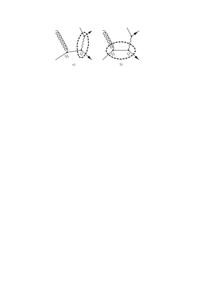
Figure 1: Two possible cluster configurations of a W+1 jet event. The dashed line highlights the hard $2\to 2$ process.

Possible configurations resulting from the clustering of $W+1$jet events are exhibited in Fig. 1. The hard $2\to 2$ process either is again a Drell–Yan process (Fig. 1a) or of the type $q\bar{q}^{\prime}\to gW$ (Fig. 1b). The weight in the first case reads:

$${\cal W}=\Delta_{q}(Q,Q_{\rm cut})\,\Delta_{\bar{q}^{\prime}}(Q,Q_{\rm cut})\,\Delta_{g}(Q_{1},Q_{\rm cut})\frac{\alpha_{s}(Q_{1})}{\alpha_{s}(Q_{\rm cut})}\;,$$ (10)

where $Q^{2}=M_{e\bar{\nu}_{e}}^{2}$ and the nodal value $Q_{1}$ is given by the $k_{\perp}$-algorithm. For this configuration the gluon jet tends to be soft, i.e. $Q_{1}$ preferentially is close to $Q_{\rm cut}$. The second configuration differs from the first only by the result of the clustering. The transverse momentum of the gluon jet $p_{\perp,g}^{2}$ now is of the order of the $W$-boson mass or larger. The weight looks still the same only the scale definitions are altered. In such a case, the hard scale is now given by

$$Q^{2}=p_{\perp,g}^{2}+M_{e\bar{\nu}_{e}}^{2}\,,$$ (11)

i.e. the transverse mass of the $W$. Also, the nodal value $Q_{1}$ has not been determined by the cluster algorithm, since it belongs to the (in principle unresolved) core process. A natural choice is the transverse momentum of the corresponding jet

$$Q_{1}=p_{\perp,g}\;.$$ (12)

These scale definitions guarantee a smooth transition between the two regimes, i.e. from the case where the gluon is soft to a case where the gluon is hard.

More complicated processes involve the production of at least two extra jets. There are many processes contributing to this category. Some illustrative examples are displayed in Fig. 2.

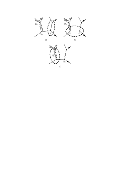
Figure 2: Three possible cluster configurations of a W+2 jet event. The dashed line highlights the hard $2\to 2$ process, being either of Drell–Yan type (a), a vector boson production (b) or a pure QCD process (c).

Cases a) and b) of Fig. 2 are very similar to the example with one extra jet only. The corresponding weight reads:

$${\cal W}=\Delta_{q}(Q,Q_{\rm cut})\,\Delta_{\bar{q}^{\prime}}(Q,Q_{\rm cut})\,\Delta_{g}(Q_{1},Q_{\rm cut})\,\Delta_{g}(Q_{2},Q_{\rm cut})\frac{\alpha_{s}(Q_{1})}{\alpha_{s}(Q_{\rm cut})}\,\frac{\alpha_{s}(Q_{2})}{\alpha_{s}(Q_{\rm cut})}\;.$$ (13)

The nodal value $Q_{2}$ is given by the $k_{\perp}$-algorithm. The scales $Q_{1}$ and $Q$ are chosen as in the one-jet case.

In contrast a new situation arises when a pure QCD process has been chosen as the “core” $2\to 2$ process, see Fig. 2c). Since the “core” process is not resolved, there is only one scale available, $Q^{2}=(2stu)/(s^{2}+t^{2}+u^{2})\approx p_{\perp}^{2}$, the transverse momentum of the outgoing jets. The correction weight consequently reads:

$${\cal W}=\Delta_{q}(Q,Q_{\rm cut})\,\frac{\Delta_{q}(Q,Q_{\rm cut})}{\Delta_{q}(Q_{1},Q_{\rm cut})}\,\Delta_{\bar{q}^{\prime}}(Q_{1},Q_{\rm cut})\,[\Delta_{g}(Q,Q_{\rm cut})]^{2}\left[\frac{\alpha_{s}(Q)}{\alpha_{s}(Q_{\rm cut})}\right]^{2}\,.$$ (14)

The extension to higher multiplicities is straightforward. However, the number of extra jets accounted for by matrix elements is limited. This limitation in available MEs enforces a specific treatment of the processes with the highest multiplicity.

II.4 The highest multiplicity treatment

In general, the initial cross sections $\sigma^{(0)}_{i}$ used in step 1 of the merging algorithm above are defined by

$$\sigma^{(0)}_{i}=\int dx_{1}\,dx_{2}\,d\Omega\;f_{1}(x_{1},\mu_{F})f_{2}(x_{2},\mu_{F})\left|{\cal M}_{i}\right|^{2}\,,$$ (15)

where $d\Omega$ represents the appropriate invariant phase-space element and ${\cal M}_{i}$ is the Feynman amplitude for the respective process. The choice $\mu_{F}=Q_{\rm cut}$ together with the Sudakov factors and the coupling weight leads to a modified cross section $\sigma_{i}={\cal W}\,\sigma^{(0)}_{i}$. Adding all cross sections with the same number of strong particles yields the cross section for production processes accompanied by – exclusively – $n$ jets,

$$\sigma_{n-jet}^{({\rm excl})}=\sum_{i(n\,jet)}\sigma_{i}\;.$$ (16)

Of course the number of extra jets that can be considered in this respect is limited by the available matrix elements; in SHERPA, this number is usually in the range of three to four. In order to compensate for all the omitted processes with more jets, the treatment of processes with the highest number of extra jets differs slightly from the handling of lower jet multiplicities. The changes are as follows:

• the factorisation scale is set dynamically to $\mu_{F}=Q_{\rm min}$, i.e. to the smallest nodal value as determined by the $k_{\perp}$-algorithm,

• the resolution scale $Q_{\rm cut}$ of the Sudakov weights is also replaced by $Q_{\rm min}$, and

• the shower veto is applied with $Q_{\rm min}$ instead of $Q_{\rm cut}$.

This guarantees that parton showers attached to matrix elements with the highest number of jets are allowed to produce softer jets. In other words: the merging procedure is meant to take into account quantum interference effects in jet production at leading order up to a maximal number of jets; any softer jet is left to the parton shower. For the configuration shown in Fig. 2a), the modified Sudakov and coupling weight reads:

$$\tilde{\cal W}=\Delta_{q}(Q,Q_{\rm min})\,\Delta_{\bar{q}^{\prime}}(Q,Q_{\rm min})\,\Delta_{g}(Q_{1},Q_{\rm min})\,\frac{\alpha_{s}(Q_{1})}{\alpha_{s}(Q_{\rm cut})}\,\frac{\alpha_{s}(Q_{2})}{\alpha_{s}(Q_{\rm cut})}\;,$$ (17)

with lowest scale $Q_{\rm min}=Q_{2}$. Following this procedure, the sum of all cross sections $\tilde{\sigma}_{i}=\tilde{\cal W}\,\tilde{\sigma}^{(0)}_{i}$ for a number of jets $n$ can be interpreted as an inclusive cross section

$$\sigma_{n-jet}^{({\rm incl})}=\sum_{i(n\,jet)}\tilde{\sigma}_{i}\;,$$ (18)

i.e. the probability to find at least $n$ jets. Adding all exclusive cross sections for multiplicities lower than a maximal multiplicity $n_{\rm max}$ to the inclusive cross section for the highest multiplicity results in a fully inclusive cross section.

II.5 On-shell matrix elements vs. off-shell parton shower kinematics

One subtle problem when combining matrix elements with parton showers is connected to the question of how to translate the matrix element kinematics, determined with on-shell (for light quarks usually massless) momenta, into a kinematics suitable for the virtuality-ordered parton shower, i.e. invoking off-shell momenta. Within the SHERPA framework, this problem is dealt with by the parton shower in the usual fashion: to begin with, the energy fraction $z$ is determined from on-shell kinematics, and afterwards it is reinterpreted. For details on the virtuality-ordered parton in SHERPA, the reader is referred to a forthcoming publication apacic-2-0 . However, if no further emissions are added through the parton shower, the partons stemming from the matrix element are left on their mass-shell and the kinematics remains unaltered. On the other hand, if the virtuality of one or more partons from the matrix element is increased through secondary emissions induced by the shower, the kinematics is modified. Usually, the scales involved in the showering are much smaller than the scales prevalent in the matrix elements, which are of the order of or larger than $Q_{\rm cut}$. Consequently, any manipulation of the kinematics tends to be mild. Nevertheless in some cases changes in the kinematics may lead a posteriori to a considerable change of the nodal values from the $k_{\perp}$-algorithm. For instance, the production of $W$ bosons at the Tevatron exhibits a strong asymmetry, which, to a considerable fraction, leads to configurations of the initial state, where the emission of jets or extra partons is concentrated on one incoming parton only. On rare occasions, such mass effects may alter the smallest nodal value in such a way that it becomes smaller than $Q_{\rm cut}$. In these cases, the phase-space separation underlying the full merging procedure is violated. Within the SHERPA framework, these events are rejected. The corresponding rejection procedure is such that

• the next event is of the same process as the one being rejected, and

• the Sudakov weight is only applied to correct the kinematics rather than the rates.

Therefore, the jet rates determined by the prescription given in the previous section are not altered by the parton shower, and the phase-space separation through the $k_{\perp}$-algorithm is enforced.

III Consistency checks

In this section the self-consistency of the results obtained with SHERPA is checked by analysing the dependence of different observables on the key parameters of the merging procedure, namely the separation scale $Q_{\rm cut}$ and the highest multiplicity of included matrix elements $n_{\rm max}$. All plots in this section correspond to $W^{-}$ boson production at the Tevatron, Run II; the parameter settings can be found in the Appendix. If not stated otherwise, the distributions shown are inclusive hadron level results, i.e. no cuts have been applied.

III.1 Variation of the separation cut $Q_{\rm cut}$

In all figures, the black, solid line represents the total inclusive result as obtained by SHERPA. A vertical dashed line indicates the respective separation cut $Q_{\rm cut}$, which has been varied between 10 GeV and 50 GeV. To guide the eye, all plots also show the same observable as obtained with a separation cut $Q_{\rm cut}=20$ GeV, shown as a dashed black curve. The coloured lines give the contributions of different multiplicity processes. Note that the separation cut always marks the transition between $n$-jet and $n+1$-jet matrix elements.

Figure 3: $p_{\perp}(W^{-})$ and $p_{\perp}(e^{-})$ for $Q_{\rm cut}=10$ GeV, $30$ GeV and $50$ GeV in comparison with $Q_{\rm cut}=20$ GeV.

Figure 4: $\eta(W^{-})$ and $\eta(e^{-})$ for $Q_{\rm cut}=10$ GeV, $30$ GeV and $50$ GeV in comparison with $Q_{\rm cut}=20$ GeV.

Figs. 3 and 4 show the transverse momentum and the rapidity distribution of the $W^{-}$ boson and the corresponding electron. For the transverse momentum of the $W$ below the cut, the distribution is dominated by the LO matrix element with no extra jet, i.e. the transverse momentum is generated by the initial state parton shower only. Around the cut, a small dip is visible in Fig. 3. The $p_{\perp}$ distribution of the electron, in contrast, is hardly altered. The rapidity distributions in Fig. 4 exhibit the asymmetry, which has been anticipated when considering merely the negatively charged $W$ boson. The shape of these distributions is very stable under a variation of the separation cut. In all observables a small increase of the total cross section of a few percent when changing $Q_{\rm cut}$ from 10 GeV to 50 GeV is visible. This underlines the fact that the dependence on the separation cut is weak.

Figure 5: Differential jet rates for the $1\to 0$, $2\to 1$ and $3\to 2$ transition (top to bottom), for
$Q_{\rm cut}=10$ GeV, $30$ GeV, and $50$ GeV (from left to right). In each plot, the results are compared with those for $Q_{\rm cut}=20$ GeV.

Differential jet rates with respect to the $k_{\perp}$-algorithm are interesting observables, since they basically exhibit the distributions of nodal values using the cluster algorithm. For simplicity the Run II $k_{\perp}$-algorithm has been used with $D=1$ for the analysis. Differential jet rates are of special interest, since the nodal values are very close to the measure used to separate matrix elements from parton shower emissions. Some minor problems with respect to the separation should immediately manifest themselves in these distributions. In Fig. 5 the $1\to 0$, $2\to 1$ and $3\to 2$ differential jet rates are shown. Within the given approximation the independence is satisfactory.

III.2 Variation of the maximal jet multiplicity $n_{\rm max}$

For very inclusive observables such as transverse momentum and rapidity of the $W$ boson, it is usually sufficient to include the matrix element with only one extra jet in order to obtain a reliable prediction. Consequently, the inclusion of matrix elements with more than one extra jet in the simulation should not significantly change the result. This can be used as another consistency check. Figs. 6 and 7 impressively picture the dependence on the maximal jet number in the matrix elements included. They show that the treatment of the highest multiplicity (cf. Sec. II.4) completely compensates for the missing matrix elements, whereas the contribution of the lowest multiplicity is not altered.

Figure 6: $p_{\perp}(W^{-})$ for $Q_{\rm cut}=15$ GeV and different maximal numbers of ME jets included.

Figure 7: $\eta(W^{-})$ for $Q_{\rm cut}=15$ GeV and different maximal numbers of ME jets included.

III.3 Matrix element, parton shower and hadronisation

In addition to the self-consistency of the algorithm tested so far at the hadron level, it is worth while to check that the parton shower and hadronisation do not induce significant changes with respect to the initial reweighted matrix element in high-$p_{\perp}$ regions. Fig. 8 proves that the predictions of SHERPA, e.g. the $p_{\perp}$ distribution of the hardest jet in $W$ production, are remarkably stable in the region of matrix element dominance.

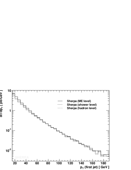
Figure 8: The $p_{\perp}$ of the hardest jet in inclusive $W$ production at the Tevatron, Run II. The solid line indicates the distribution as delivered by the matrix elements; the dashed line is obtained after parton shower evolution; and the dotted line gives the final result after hadronisation. Here $Q_{\rm cut}=15$ GeV.

III.4 Variation of factorisation and renormalisation scale

Finally, the sensitivity of the previous results with respect to changes in the renormalisation and factorisation scale are examined. In the following all scales occurring in the event generation, both on the matrix element and at the parton shower level, are multiplied by constant factors, ranging from $0.5$ up to $5$. It is clear that the total cross section changes with changing scales: starting with 930 pb for the default scale choice, 887 pb (959 pb) are obtained when using a scale factor of 0.5 (2). The shape of the $p_{\perp}$ distributions of the jets, however, experiences only mild changes. This is greatly exemplified by the left panel of Fig. 9, where the $p_{\perp}$ spectrum of the hardest jet is displayed. In the right panel of Fig. 9 the result of the left panel is broken down for two different scale prefactors, $1$ and $5$, to the different contributions. Clearly, at the individual level different jet multiplicities differ also in their shapes; in their interplay, however, these effects cancel in terms of the overall shape.

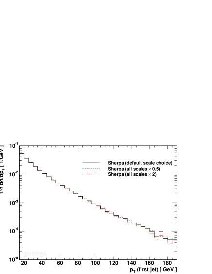
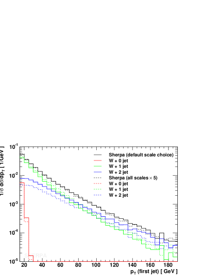
Figure 9: The $p_{\perp}$ of the hardest jet in inclusive $W$ production at the Tevatron, Run II, and its dependence on different choices in the renormalisation and factorisation scale. In the left plot, the solid line indicates the default hadron level result; the green dashed and the red dotted line are obtained by multiplying all scales in the coupling constants and the PDFs in both the matrix elements and the parton shower by a factor of $0.5$ or $2$, respectively. In the right plot, the same observable is investigated in more detail with the default scales (solid lines) and with all scales multiplied by a factor of $5$. In addition the different contributions of different jet multiplicities are shown.

IV SHERPA vs. data and other MCs

In order to study the impact of the merging prescription, the predictions obtained with SHERPA may also be compared with other approaches. In a first step, in Sec. IV.1 the transverse momentum distribution of the first and second hardest jets in exclusive and inclusive boson-plus-jet production from SHERPA are confronted with the NLO QCD predictions of the parton level generator MCFM Campbell:2002tg ; Campbell:2003hd . In Sec. IV.2 the full event generators MC@NLO Frixione:2004wy and PYTHIA Sjostrand:2003wg are used to investigate the capabilities of SHERPA when studying $W/Z$+jet production at the hadron level. Finally Sec. IV.3 contains a comparison of the predictions made for the bosons transverse momentum distribution with those measured by the D0 and CDF collaborations at the Tevatron, Run I.

IV.1 SHERPA vs. MCFM

In order to compare the SHERPA predictions for $W/Z$+1jet and $W/Z$+2jet production, a two-step procedure is chosen. In a first step the Sudakov and $\alpha_{s}$ reweighted matrix elements are compared with exclusive NLO results obtained with MCFM. In the case of the next-to-leading order calculation, the exclusiveness of the final states boils down to a constraint on the phase space for the real parton emission. The exclusive SHERPA results consist of appropriate leading order matrix elements with scales set according to the $k_{\perp}$-clustering algorithm and made exclusive by suitable Sudakov form factors, cf. Sec. II.2. In a second step, the jet spectra for inclusive production processes are compared. For the next-to-leading order calculation, this time the phase space for real parton emission is not restricted and the SHERPA predictions are obtained from a fully inclusive sample, using matrix elements with up to two extra jets and the parton showers attached. If not stated otherwise, all results have been obtained using the input parameters and phase-space cuts summarised in the Appendix. Jets are found using the Run II $k_{\perp}$-clustering algorithm defined in Blazey:2000qt with a pseudo-cone size of $D=0.7$ and a minimal $p_{\perp}$ of $15$ GeV.

IV.1.1 Exclusive jet $p_{\perp}$ spectra

In Fig. 10 the jet $p_{\perp}$ distribution for the exclusive production of $W$+1jet and $Z$+1jet are shown. In both figures, the SHERPA prediction is compared with the exclusive NLO result obtained with MCFM and with the naive LO prediction, which is the same for the two programs. For the fixed-order NLO and LO result, the renormalisation and factorisation scales have been set to $\mu_{R}=\mu_{F}=80.419\;{\rm GeV}=M_{W}$. All distributions have been normalised to the corresponding total cross section. This allows for a direct comparison of the distributions shape. As stated above, the SHERPA results stem from Sudakov and $\alpha_{s}$ reweighted $W$+1jet or $Z$+1jet LO matrix elements. The change between the naive leading order and the next-to-leading order distribution is significant. At next-to-leading order the distributions become much softer. For a high-$p_{\perp}$ jet it is much more likely to emit a parton that fulfils the jet criteria and therefore removes the event from the exclusive sample. The SHERPA predictions show the same feature. The inclusion of Sudakov form factors and the scale setting according to the merging prescription improves the LO prediction, resulting in a rather good agreement with the next-to-leading order result.

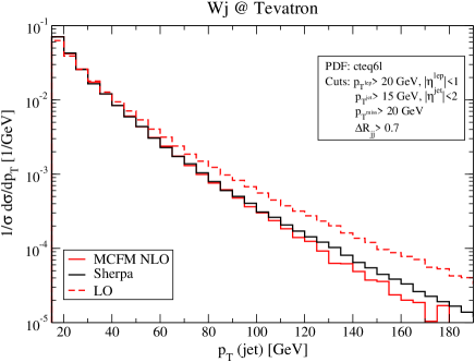
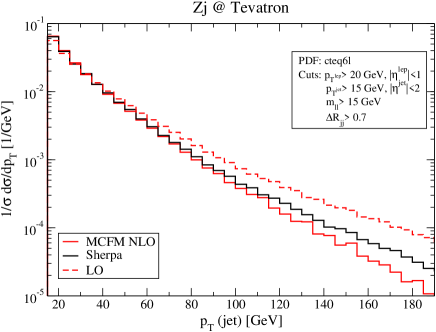
Figure 10: Jet $p_{\perp}$ distribution of exclusive $W+1$jet (left) or $Z+1$jet (right) events at the Tevatron, Run II.

In the high-$p_{\perp}$ tail, however, the NLO calculations from MCFM tend to be a bit below the SHERPA results. The reason is simply connected to the fact that relevant scales in the high-$p_{\perp}$ tail are much larger than the default choice of $\mu_{R}=\mu_{F}=80.419$ GeV. In order to highlight this, Fig. 11 contains the jet $p_{\perp}$ distribution in $Z$+1jet events. In this plot, the renormalisation and factorisation scales have been chosen to be $\mu_{R}=\mu_{F}=160.838\;{\rm GeV}=2M_{W}$. Changing the scale in this manner indeed has quite a small impact on the total cross section at NLO, but the tail of the distribution becomes considerably enhanced. With the above choice of $\mu_{R}$ and $\mu_{F}$ the agreement of NLO and the SHERPA result is impressive.

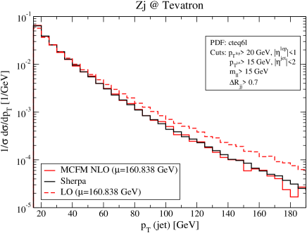
Figure 11: Jet $p_{\perp}$ distribution of $Z+1$jet events at the Tevatron where for the NLO and LO calculation the renormalisation and factorisation scales have been chosen to be $\mu_{R}=\mu_{F}=160.838$ GeV.

The $p_{\perp}$ distribution of the first and second jets in $W$+2jet and $Z$+2jet production are presented in Fig. 12. Again, the next-to-leading oder distributions are softer than the leading order ones, for the same reason as for the 1jet case. In addition, at low-$p_{\perp}$ the leading order result is smaller than the next-to-leading order one. Taken together, the curves have a significantly different shape over the whole interval. This situation clearly forbids the use of constant $K$-factors in order to match the leading order with the next-to-leading order result. Nevertheless, as before, the SHERPA prediction reproduces to a very good approximation the shape of the NLO result delivered by MCFM. Fig. 13 shows that, similar to the $Z$+1jet case for $W$+2jet in the high-$p_{\perp}$ tail, the situation is even better using higher renormalisation and factorisation scales (e.g. $\mu_{R}=\mu_{F}=160.838$ GeV) in the NLO calculation.

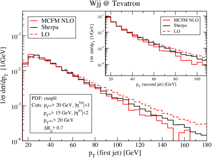
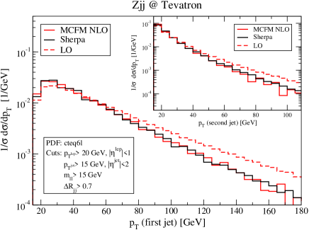
Figure 12: The $p_{\perp}$ distribution of the first and second jets in exclusive $W+2$jet (left) and in exclusive $Z+2$jet (right) events at the Tevatron, Run II.

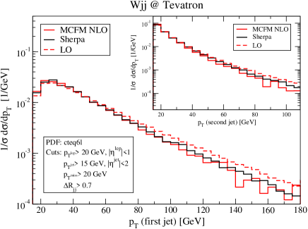
Figure 13: The $p_{\perp}$ distribution of the first and second jets in exclusive $W+2$jet events at the Tevatron where for the NLO and LO calculation the renormalisation and factorisation scales have been chosen to $\mu_{R}=\mu_{F}=160.838$ GeV.

IV.1.2 Inclusive jet $p_{\perp}$ spectra

NLO results for inclusive boson plus jet(s) production obtained with MCFM are compared with fully inclusive samples generated with SHERPA. There, the matrix elements for $W/Z$+0,1,2jet production have been used including the highest multiplicity treatment for the $W/Z$+2jet case. The Sudakov and $\alpha_{s}$ reweighted matrix elements have now been combined with the initial and final state parton showers. The hadronisation phase for the SHERPA events has been discarded. As for the exclusive case the naive leading order prediction is given by the corresponding leading order matrix element that is identical to the one in Figs. 10 and 12. For the NLO prediction again the renormalisation and factorisation scales have been chosen to coincide, namely $\mu_{R}=\mu_{F}=80.419$ GeV.

In Fig. 14, the $p_{\perp}$ spectra for the hardest jet in inclusive $W/Z$+1jet production are shown. Compared with the exclusive predictions, the high-$p_{\perp}$ tail is filled again and, hence, the differences between the NLO calculations and the LO ones appear to be smaller. For both cases the SHERPA result and the NLO calculation are in good agreement.

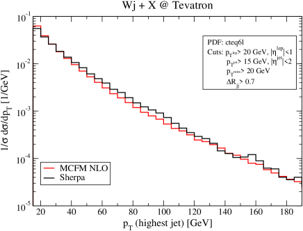
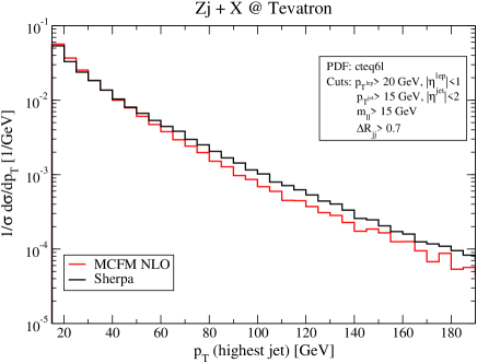
Figure 14: The $p_{\perp}$ distribution of the hardest jet for inclusive $W+1$jet (left) and for inclusive $Z+1$jet (right) production at the Tevatron, Run II.

In Fig. 15 the $p_{\perp}$ spectra for the first and second hardest jets in inclusive $W/Z$+2jet production are presented. Considering the scale dependence of the next-to-leading order result in the high-$p_{\perp}$ region, as already studied in Fig. 13 for the exclusive result, the curves are in pretty good agreement.

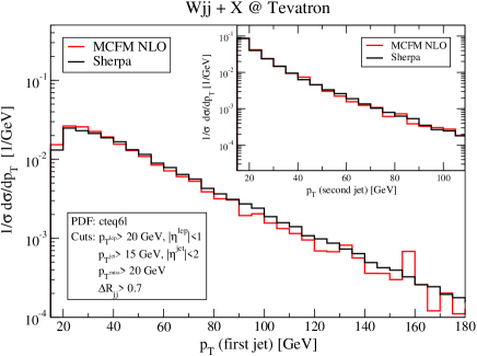
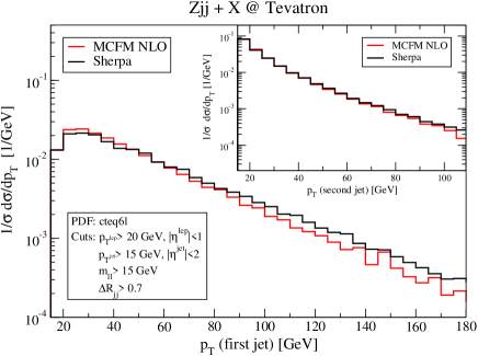
Figure 15: The $p_{\perp}$ distribution of the hardest two jets for inclusive $W+2$jet (left) and for inclusive $Z+2$jet (right) production at the Tevatron, Run II.

Altogether, the merging procedure in SHERPA, including the scale-setting prescription of the approach and the Sudakov reweighting of the LO matrix elements, proves to lead to a significantly improved leading order prediction. Seemingly, it takes proper care of the most relevant contributions of higher order corrections. Although it should be stressed that the rate predicted by SHERPA is still a leading order value only, a constant $K$-factor is sufficient to recover excellent agreement with a full next-to-leading order calculation for the distributions considered. Furthermore, by looking at the inclusive spectra it is obvious that this statement still holds true after the inclusion of parton showers and the merging of exclusive matrix elements of different jet multiplicities.

IV.2 SHERPA vs. MC@NLO and PYTHIA

In a next step, results obtained with SHERPA are compared with those obtained from two other event generators, namely PYTHIA and MC@NLO. In both, standard settings have been used for inclusive $W$ production at the Tevatron and the underlying event has been switched off. The corresponding process number in PYTHIA is MSEL=12, the relevant MC@NLO process is IPROC=-1471. Inclusive quantities like, for instance, the $p_{\perp}$ and $\eta$ distributions of the $W$ are in good agreement, see Fig. 16, and only in the high-$p_{\perp}$ tail of the distribution some small deviations become visible. However, more exclusive quantities such as the $p_{\perp}$-distributions of the first three jets show differences that increase with the increasing order of the jet. This can clearly be seen from Fig. 17. The predictions for the hardest jet start to disagree with a factor of roughly 2 at jet-$p_{\perp}$s of the order of 100 GeV, reaching up to nearly an order of magnitude at $p_{\perp}$ around 200 GeV. This trend is greatly enhanced for the second and third jets, where discrepancies are of the order of one magnitude for the second jet at $p_{\perp}\approx 100$ GeV or even higher for the third jet.

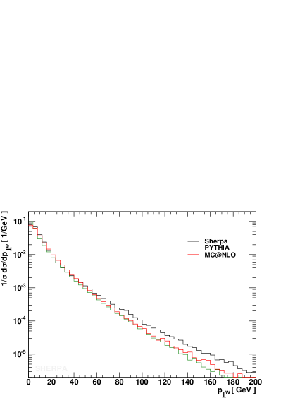
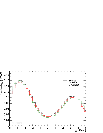
Figure 16: The $p_{\perp}$ (left) and $\eta$ (right) distribution of the $W^{-}$ boson for inclusive production at the Tevatron, Run II. Plotted are the results as obtained with the generators PYTHIA (green), MC@NLO (red) and SHERPA (black).

These discrepancies, however, were to be expected since the other two programs do not include any higher order correction beyond first order in the strong coupling constant. In the case of MC@NLO, predictions have been compared with those obtained from MCFM; after a careful calibration of input parameters such as CKM elements etc., inside the code both programs coincided in all observables tested Frixione:private . Therefore, differences in the $p_{\perp}$ distribution of the hardest jet have to be attributed to a combination of distinct parameter settings and of differences in parton showering and hadronisation. The latter type of difference should be taken as some kind of theoretical uncertainty. For higher jet configurations, however, the remaining discrepancies are due to different physics input.

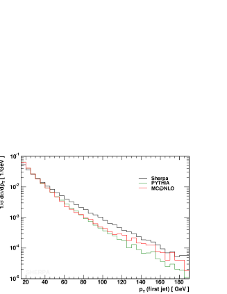
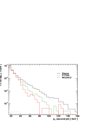
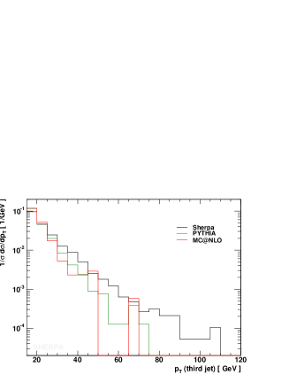
Figure 17: Jet $p_{\perp}$ distribution of the three hardest jets in inclusive $W$ production at the Tevatron, Run II. Compared are the hadron level results of SHERPA (black), PYTHIA (green) and MC@NLO (red) after 2.5 million events.

IV.3 SHERPA vs. data

Having compared the SHERPA predictions for the case of the jet transverse momentum distributions in exclusive and inclusive $W/Z$+1jet and $W/Z$+2jet production against other Monte Carlo programs, a comparison with experimental data provides an ultimate test of SHERPA’s ability to describe such processes. Unfortunately, so far only the inclusive $W$- and $Z$-boson transverse momentum distribution measured in Tevatron, Run I, have been published, which allows for an overall check only. In both cases, matrix elements with up to four ($W$) or three ($Z$) extra jets have been taken into account – as indicated by the different colours - to generate the SHERPA sample. The black line represents the sum of all contributions. For this sample the required separation cut has been chosen to $Q_{\rm cut}=20$ GeV.

In Fig. 18, the (inclusive) $p_{\perp}$ distribution of the $W$ is compared with data from D0, taken at Run I of the Tevatron Abbott:2000xv . The agreement with data is excellent. It can be recognised that approaching the merging scale from below, the $W$+0jet contribution steeply falls and the distribution for larger momenta is mainly covered by the $W$+1jet part, as expected. In order to match the measured distribution, the SHERPA result has been multiplied by a constant $K$-factor of $1.25$.

Similarly, in Fig. 19, the (inclusive) $p_{\perp}$ distribution of the $Z$ is compared with data, this time taken by CDF at Run I of Tevatron Affolder:1999jh . Again the overall agreement is excellent. This time the result has been multiplied by a constant $K$-factor of $1.6$ to match the data. The result is perfectly smooth around the merging scale of $Q_{\rm cut}=20$ GeV. This is especially highlighted in the left plot of Fig. 19, which concentrates on the low momentum region. It is interesting to note that the description of the data for momenta smaller than the merging scale is almost only covered by the $Z$+0jet contribution and is therefore very sensitive to the details of the parton showers and the treatment of beam remnants. A parameter of specific impact on the very low momentum region therefore is the primordial (or intrinsic) $k_{\perp}$ used for the interacting partons. This is modelled through a Gaussian distribution with a central value of $0.8$ GeV. Nevertheless, the shower performance of SHERPA has not been especially tuned; the low momentum behaviour may therefore still be improved once a detailed parameter tune is available.

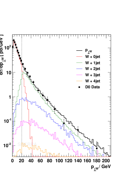
Figure 18: The $p_{\perp}$ distribution of the $W$-boson in comparison with data from D0 at the Tevatron, Run I Abbott:2000xv . The total result is indicated by the black line. The coloured lines show the contributions of the different multiplicity processes. Here matrix elements with up to four extra jets have been considered. The applied separation cut is $Q_{\rm cut}=20$ GeV.

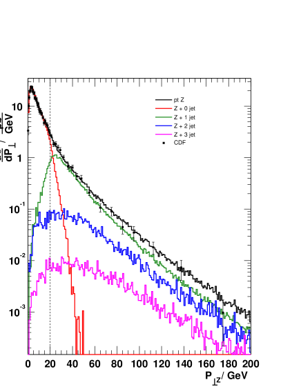
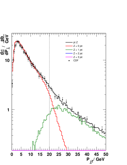
Figure 19: The $p_{\perp}$ distribution of the $Z$-boson in comparison with data from CDF at the Tevatron, Run I Affolder:1999jh . The total result is indicated by the black line. The coloured lines show the contributions of the different multiplicity processes. The applied separation cut is $Q_{\rm cut}=20$ GeV. The right plot focuses on the low momentum region of the left one.

V Conclusion

In this work, predictions for single-boson production processes at the Tevatron have been obtained from the new event generator SHERPA and compared with the results from other programs and with data. In all cases an encouraging agreement of results has been found. Especially for the description of exclusive multi particle final states, SHERPA proved its unique value as the simulation tool of choice, limited only by the maximal number of external particles covered by its intrinsic matrix elements. In practical applications the choice of this input should be guided by the question in consideration. For instance, for the simulation of $W+4$jet background to top pair production, a highest jet multiplicity of 4 is advisable in order to include most of the quantum interferences.

Having validated the versatility of SHERPA on one of the most important processes at hadron colliders, its abilities will be further tested in the near future by considering other important processes, such as the production of boson pairs, the Higgs boson, heavy quarks, or multijet final states.

Appendix A Input parameters and phase-space cuts

The PDF set used for all analyses is cteq6l Pumplin:2002vw . The value of $\alpha_{s}$ is chosen according to the value taken for the PDF, namely $0.118$. For the running of the strong coupling the corresponding two-loop equation is used. Jets or initial partons are restricted to the light flavour sector, namely $g,u,d,s,c$. In fact these flavours are taken to be massless and the Yukawa couplings of the quarks are neglected throughout the entire analysis.

A.0.1 SM input parameters

The SM parameters are given in the $G_{\mu}$ scheme:

$$m_{W}=80.419\;{\rm GeV}\,,\quad\Gamma_{W}=2.06\;{\rm GeV,}$$

$$m_{Z}=91.188\;{\rm GeV}\,,\quad\Gamma_{Z}=2.49\;{\rm GeV,}$$

$$G_{\mu}=1.16639\times 10^{-5}\;{\rm GeV}^{-2},$$

$$\sin^{2}\theta_{W}=1-m^{2}_{W}/m^{2}_{Z}=0.2222,$$

$$\alpha_{s}=0.118\,.$$ (19)

The electromagnetic coupling is derived from the Fermi constant $G_{\mu}$ according to

$$\alpha_{\rm em}=\frac{\sqrt{2}\,G_{\mu}\,M^{2}_{W}\,\sin^{2}\theta_{W}}{\pi}=1/132.51\,.$$ (20)

The constant widths of the electroweak gauge bosons are introduced via the fixed-width scheme. CKM mixing of the quark generations is neglected.

A.0.2 Cuts and jet criteria

For all jet analyses the Run II $k_{\perp}$-clustering algorithm defined in Blazey:2000qt is used. The parameter of this jet algorithm is a pseudo-cone of size $D$ given below for the Tevatron analysis. For the charged leptons the following cuts are applied:

$$p^{\rm lepton}_{\perp}>20\;{\rm GeV},\quad|\eta^{\rm lepton}|<1,\quad m^{ll}>15\;{\rm GeV}.$$ (21)

For the case of $W$ production an additional cut on missing transverse momentum according to the neutrino has been required, namely

$$p^{\rm miss}_{\perp}>20\;{\rm GeV}.$$ (22)

For the jet definition a pseudo-cone size of $D=0.7$ has been used in addition to cuts on pseudo-rapidity and transverse momentum:

$$p_{\perp}^{\rm jet}>15\;{\rm GeV},\quad|\eta^{\rm jet}|<2.$$ (23)

References

- (1) S. Abachi et al. [D0 Collaboration], Phys. Rev. Lett. 75 (1995) 1456 [arXiv:hep-ex/9505013].
- (2) T. Affolder et al. [CDF Collaboration], Phys. Rev. D 64 (2001) 052001 [arXiv:hep-ex/0007044].
- (3) V. M. Abazov et al. [D0 Collaboration], Phys. Rev. D 66 (2002) 012001 [arXiv:hep-ex/0204014].
- (4) W. Ashmanskas et al., the Tevatron Electroweak Working Group, CDF and D0 Collaborations, arXiv:hep-ex/0311039.
- (5) C. Albajar et al. [UA1 Collaboration], Phys. Lett. B 253 (1991) 503.
- (6) J. Alitti et al. [UA2 Collaboration], Phys. Lett. B 276 (1992) 365.
- (7) F. Abe et al. [CDF Collaboration], Phys. Rev. D 52 (1995) 2624.
- (8) B. Abbott et al. [D0 Collaboration], Phys. Rev. D 61 (2000) 072001 [arXiv:hep-ex/9906025].
- (9) T. Affolder et al. [CDF Collaboration], Phys. Rev. Lett. 85 (2000) 3347 [arXiv:hep-ex/0004017].
- (10) V. M. Abazov et al. [D0 Collaboration], Phys. Rev. D 66 (2002) 032008 [arXiv:hep-ex/0204009].
- (11) S. Haywood et al., arXiv:hep-ph/0003275.
- (12) ATLAS Collaboration, “Detector and Physics Performance Technical Design Report”, CERN/LHCC/99-15, vol. 2.
- (13) V. A. Khoze, A. D. Martin, R. Orava and M. G. Ryskin, Eur. Phys. J. C 19 (2001) 313 [arXiv:hep-ph/0010163].
- (14) M. Dittmar, F. Pauss and D. Zurcher, Phys. Rev. D 56 (1997) 7284 [arXiv:hep-ex/9705004].
- (15) A. D. Martin, R. G. Roberts, W. J. Stirling and R. S. Thorne, Eur. Phys. J. C 14 (2000) 133 [arXiv:hep-ph/9907231].
- (16) W. T. Giele and S. A. Keller, arXiv:hep-ph/0104053.
- (17) G. Altarelli, R. K. Ellis and G. Martinelli, Nucl. Phys. B 157 (1979) 461.
- (18) J. Kubar-Andre and F. E. Paige, Phys. Rev. D 19 (1979) 221.
- (19) K. Harada, T. Kaneko and N. Sakai, Nucl. Phys. B 155 (1979) 169 [Erratum, ibid. B 165 (1980) 545].
- (20) J. Abad and B. Humpert, Phys. Lett. B 80 (1979) 286.
- (21) B. Humpert and W. L. Van Neerven, Phys. Lett. B 85 (1979) 293.
- (22) R. Hamberg, W. L. van Neerven and T. Matsuura, Nucl. Phys. B 359 (1991) 343 [Erratum, ibid. B 644 (2002) 403].
- (23) R. V. Harlander and W. B. Kilgore, Phys. Rev. Lett. 88 (2002) 201801 [arXiv:hep-ph/0201206].
- (24) C. Anastasiou, L. Dixon, K. Melnikov and F. Petriello, arXiv:hep-ph/0312266.
- (25) C. Balazs and C. P. Yuan, Phys. Rev. D 56 (1997) 5558 [arXiv:hep-ph/9704258].
- (26) F. A. Berends, H. Kuijf, B. Tausk and W. T. Giele, Nucl. Phys. B 357 (1991) 32.
- (27) A. Pukhov et al., arXiv:hep-ph/9908288.
- (28) T. Ishikawa, T. Kaneko, K. Kato, S. Kawabata, Y. Shimizu and H. Tanaka [MINAMI-TATEYA group Collaboration], KEK-92-19
- (29) K. Sato et al., Proc. VII International Workshop on Advanced Computing and Analysis Techniques in Physics Research (ACAT 2000), P. C. Bhat and M. Kasemann, AIP Conference Proceedings 583 (2001) 214.
- (30) T. Stelzer and W. F. Long, Comput. Phys. Commun. 81 (1994) 357 [arXiv:hep-ph/9401258];
- (31) F. Maltoni and T. Stelzer, JHEP 0302 (2003) 027 [arXiv:hep-ph/0208156].
- (32) JHEP 0307 (2003) 001 [arXiv:hep-ph/0206293].
- (33) F. Krauss, R. Kuhn and G. Soff, JHEP 0202, 044 (2002) [arXiv:hep-ph/0109036].
- (34) J. Campbell and R. K. Ellis, Phys. Rev. D 65 (2002) 113007 [arXiv:hep-ph/0202176].
- (35) J. Campbell, R. K. Ellis and D. L. Rainwater, Phys. Rev. D 68 (2003) 094021 [arXiv:hep-ph/0308195].
- (36) T. Sjöstrand, Comput. Phys. Commun. 82 (1994) 74;
- (37) T. Sjöstrand, L. Lönnblad, S. Mrenna and P. Skands, arXiv:hep-ph/0308153.
- (38) G. Corcella et al., JHEP 0101 (2001) 010 [arXiv:hep-ph/0011363].
- (39) G. Corcella et al., arXiv:hep-ph/0210213.
- (40) G. Miu and T. Sjöstrand, Phys. Lett. B 449 (1999) 313 [hep-ph/9812455].
- (41) M. H. Seymour, Comput. Phys. Commun. 90 (1995) 95 [hep-ph/9410414].
- (42) G. Corcella and M. H. Seymour, Nucl. Phys. B 565 (2000) 227 [hep-ph/9908388].
- (43) S. Frixione and B. R. Webber, JHEP 0206 (2002) 029 [arXiv:hep-ph/0204244].
- (44) S. Frixione, P. Nason and B. R. Webber, JHEP 0308 (2003) 007 [arXiv:hep-ph/0305252].
- (45) S. Frixione and B. R. Webber, arXiv:hep-ph/0402116.
- (46) S. Catani, Y. L. Dokshitzer, M. Olsson, G. Turnock and B. R. Webber, Phys. Lett. B 269 (1991) 432.
- (47) S. Catani, Y. L. Dokshitzer and B. R. Webber, Phys. Lett. B 285 (1992) 291.
- (48) S. Catani, Y. L. Dokshitzer, M. H. Seymour and B. R. Webber, Nucl. Phys. B 406 (1993) 187.
- (49) S. Catani, F. Krauss, R. Kuhn and B. R. Webber, JHEP 0111 (2001) 063 [arXiv:hep-ph/0109231].
- (50) L. Lönnblad, JHEP 0205 (2002) 046 [arXiv:hep-ph/0112284].
- (51) F. Krauss, JHEP 0208 (2002) 015 [arXiv:hep-ph/0205283].
- (52) T. Gleisberg, S. Höche, F. Krauss, A. Schälicke, S. Schumann and J. C. Winter, JHEP 0402 (2004) 056 [arXiv:hep-ph/0311263].
- (53) S. Mrenna and P. Richardson, JHEP 0405 (2004) 040 [arXiv:hep-ph/0312274].
- (54) M. L. Mangano, M. Moretti and R. Pittau, Nucl. Phys. B 632 (2002) 343 [arXiv:hep-ph/0108069].
- (55) G. C. Blazey et al., arXiv:hep-ex/0005012.
- (56) F. Krauss, A. Schälicke and G. Soff, in preparation.
- (57) S. Frixione, private communication.
- (58) B. Abbott et al. [D0 Collaboration], Phys. Lett. B 513 (2001) 292 [arXiv:hep-ex/0010026].
- (59) T. Affolder et al. [CDF Collaboration], Phys. Rev. Lett. 84 (2000) 845 [arXiv:hep-ex/0001021].
- (60) J. Pumplin, D. R. Stump, J. Huston, H. L. Lai, P. Nadolsky and W. K. Tung, JHEP 0207 (2002) 012 [arXiv:hep-ph/0201195].