Improved description of charged Higgs boson production at hadron colliders

Abstract:

We present a new method for matching the two twin-processes $gb\to H^{\pm}t$ and $gg\to H^{\pm}tb$ in Monte Carlo event generators. The matching is done by defining a double-counting term, which is used to generate events that are subtracted from the sum of these two twin-processes. In this way we get a smooth transition between the collinear region of phase space, which is best described by $gb\to H^{\pm}t$, and the hard region, which requires the use of the $gg\to H^{\pm}tb$ process. The resulting differential distributions show large differences compared to both the $gb\to H^{\pm}t$ and $gg\to H^{\pm}tb$ processes illustrating the necessity to use matching when tagging the accompanying $b$-jet.

1 Introduction

The search for physics beyond the Standard Model is one of the main objectives of the upcoming experiments at the CERN Large Hadron Collider (LHC) as well as the currently running ones at the Fermilab Tevatron. Of special interest is the scalar (Higgs) sector, which presumably is responsible for electroweak symmetry breaking and generation of particle masses. The discovery of a neutral scalar Higgs boson ($h^{0}$) would be a big step in understanding electroweak symmetry breaking. But at the same time it may be difficult to decide whether it is the Standard Model Higgs boson or if it belongs to for example a supersymmetric theory. However, the discovery of a charged Higgs boson would be a very clear signal of physics beyond the Standard Model, and would give valuable insight into the parameter space of this physics, whether supersymmetry or some other two Higgs doublet model.

Present model-independent limits on the charged Higgs boson mass from LEP are $m_{H^{\pm}}>78.6$ GeV (95% CL) [1] whereas the limits from the Fermilab Tevatron are close to $m_{H^{\pm}}\gtrsim 160\;(130)$ GeV  [2, 3] for large (small) $\tan\beta$ ($\tan\beta\gtrsim 100$ and $\tan\beta\lesssim 1$ respectively). As usual, $\tan\beta=\displaystyle\frac{v_{1}}{v_{2}}$ is the ratio of the vacuum expectation values of the two Higgs doublets which determines the coupling strength to the top and bottom quarks (roughly $\lambda_{H^{\pm}tb}\sim m_{b}\tan\beta+m_{t}\cot\beta$). For a recent review of the prospects of further charged Higgs boson searches at the Tevatron and the LHC see [4].

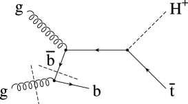
Figure 1: Illustration of the relation between the $gb\to H^{\pm}t$ and $gg\to H^{\pm}tb$ processes.

At hadron colliders, the main contribution to direct single charged Higgs boson production is through the two twin-processes $gb\to H^{\pm}t$ and $gg\to H^{\pm}tb$ . The reason for calling them twin-processes is simply that they describe the same underlying physical process, as illustrated in fig. 1, but using different approximations. In fact, the latter process enters in the next-to-leading order (NLO) calculation of the first one [5, 6, 7]. However, in the following we will concentrate on the simulation of charged Higgs boson production in Monte Carlo event generators such as Pythia [8] and Herwig [9] where only tree-processes are included. Note that although our matching procedure works for all charged Higgs masses, we are mainly interested in the region $m_{H^{\pm}}\gtrsim m_{t}-m_{b}$ where the cross-sections for the two processes are of similar size.

In the $gb\to H^{\pm}t$ process the $b$-quark is considered as a parton in the proton with a corresponding parton density which resums all the, potentially large, leading logs of the type $(\alpha_{s}\log(\mu_{F}/m_{b}))^{n}$ that arise when integrating the DGLAP evolution equation from the threshold given by the $b$-quark mass to the factorization scale $\mu_{F}$, where the proton is probed. Naturally, the treatment of the $b$-quark as a collinear massless parton in the proton leads to certain approximations which are at best only valid in the collinear limit. In contrast, the $b$-quark is not considered as a massless parton in the $gg\to H^{\pm}tb$ process and consequently the kinematics of the process are exact. This also means that the finite parts, which are not logarithmically enhanced, are also included correctly to order $\alpha_{s}^{2}$. On the other hand the $gg\to H^{\pm}tb$ process does not contain the $(\alpha_{s}\log(\mu_{F}/m_{b}))^{n}$ terms with $n>1$ which are resummed in the $b$-quark density.

In case of the total cross-section it is straightforward how to combine the $gb\to H^{\pm}t$ and $gg\to H^{\pm}tb$ processes without introducing double counting [11] (see also [12, 13]). One simply adds the cross-sections from the two processes and subtracts the common term, which is given by the $gb^{\prime}\to H^{\pm}t$ process where only the leading order logarithmically enhanced contribution to the $b$-quark density, $b^{\prime}(x,\mu_{F})\propto\alpha_{s}\log(\mu_{F}/m_{b})$ is used. In this paper we will show how this subtraction procedure can be extended also to the differential cross-section (irrespective of whether the outgoing $b$-quark is observed or not). One has to keep in mind that even though the $b$-quark is considered to be collinear in the $gb\to H^{\pm}t$ process and thereby the accompanying $b$-quark from the gluon splitting is also collinear, this is no longer true in a Monte Carlo event generator. The reason is that in the Monte Carlo, the hard process is combined with an initial state parton shower which “undoes” the DGLAP evolution back to a starting scale $Q_{0}<m_{b}$, and thereby generates an accompanying $b$-quark with non-zero $p_{\perp}$ (transverse momentum with respect to the beam axis).

The experimental techniques for detecting charged Higgs bosons rely heavily on tagging of $b$-jets and/or hadronic $\tau$-jets together with missing $p_{\perp}$. The $b$-jets can originate from the charged Higgs boson decay, the top quark decay or from an accompanying $b$-quark whereas the $\tau$-jets and missing $p_{\perp}$ of interest come from the charged Higgs boson decay. Below the top quark mass the dominating charged Higgs boson decay is $H^{\pm}\to\tau\nu_{\tau}$ whereas for heavier masses the $H\to tb$ decay mode dominates. Thus the minimum requirement is to tag one $b$-jet and either a $\tau$-jet together with missing $p_{\perp}$ or two additional $b$-jets depending on the decay mode of the charged Higgs boson. In addition the accompanying $b$-quark may also be tagged. Typical cuts used in studies by the ATLAS [14, 15] and CMS [16] collaborations for $b$-jets, $\tau$-jets and missing $p_{\perp}$ are given by the following: $p_{\perp,b}>30$ GeV, $|\eta_{b}|<2.5$, $p_{\perp,\tau}>100$ GeV, $|\eta_{\tau}|<2.5$, and $p_{\perp,\mathrm{miss}}>100$ GeV. With these cuts the $b$-tagging efficiency is of the order of $50$% with a miss-tagging rate of about 1% whereas the $\tau$-tagging efficiency is of the order of $40$% [16]. In addition the difference in polarization between a $\tau$-lepton coming from the scalar Higgs decay and the vector $W$-boson decay leads to a harder spectrum when the $\tau$ decays into one charged pion which in turn can be used to enhance the signal [17].

Conventionally the strategy, when investigating the prospects of detecting charged Higgs bosons at the LHC, has been to use the $gb\to H^{\pm}t$ process combined with parton showers when the accompanying $b$-quark is not tagged in the final state (see e.g. [14, 15]) whereas the $gg\to H^{\pm}tb$ process has been used when the $b$-quark is tagged (see e.g. [18] and [19]). As we will show in this paper, the only way to get reliable predictions in the latter case is to make a proper matching of the two processes, whereas in the first case the need for matching depends on the details of the selection used in defining the signal and the precision that one is aiming for. We will also see that in general it is not possible to simply divide the phase-space into two different parts, based for example on the $p_{\perp}$ of the accompanying $b$-quark (as in e.g. [20]), with each of them only populated by one of the processes.

The method that we present is general. The actual implementation has been done in Pythia although the same procedure could also be applied to Herwig.

The outline of the rest of the paper is as follows. We start by recalling the proper matching procedure in case of the total cross-section. In section 3 we then show how to generalize the method to be applicable also for differential cross-sections. The results of the matching procedure are presented in section 4 and in section 5 we discuss how to choose a proper factorization scale. Finally, in section 6 we give our conclusions and a short outlook.

2 The total cross-section

As already discussed in the introduction, the two different approximations describing $H^{\pm}$ production at hadron colliders that we are interested in are,

$$gb(\bar{b}) \to tH^{-}\;(\bar{t}H^{+})$$ (1)

$$gg \to t\bar{b}H^{-}\;(\bar{t}bH^{+})\quad.$$ (2)

The first one (1), which we will denote the leading order (LO) or $2\to 2$ process, includes the logarithmic DGLAP resummation of gluon splitting to $b\bar{b}$ pairs via the $b$-quark density, $b(\mu_{F}^{2})\sim\sum(\alpha_{s}\log(\mu_{F}/m_{b}))^{n}$, whereas the second one, which we will denote the $2\to 3$ process, retains the correct treatment of the accompanying $b$-quark to order $\alpha_{s}^{2}$.

In case of the total cross-section, the two approximations can be combined by simply adding them and subtracting the common term. The double-counting term which needs to be subtracted is, to leading logarithmic accuracy, given by [11]

$$\sigma_{\mathrm{DC}}=\int dx_{1}dx_{2}\left[g(x_{1},\mu_{F}^{2})b^{\prime}(x_{2},\mu_{F}^{2})\frac{d\hat{\sigma}_{2\to 2}}{dx_{1}dx_{2}}(x_{1},x_{2})+x_{1}\leftrightarrow x_{2}\right]$$ (3)

where $b^{\prime}(x,\mu_{F}^{2})$ is the leading logarithmic contribution to the $b$-quark density,

$$b^{\prime}(x,\mu_{F}^{2})=\frac{\alpha_{s}(\mu_{R}^{2})}{2\pi}\log\frac{\mu_{F}^{2}}{m_{b}^{2}}\int\frac{dz}{z}P_{g\to q\bar{q}}(z)\;g\left(\frac{x}{z},\mu_{F}^{2}\right)$$ (4)

and $P_{g\to q\bar{q}}(z)=\frac{1}{2}\left[z^{2}+(1-z)^{2}\right]$ is the splitting function.

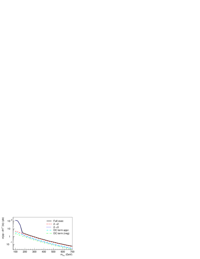
Figure 2: Integrated cross-section (components and matched total, using the exact double-counting term) as a function of the $H^{\pm}$ mass at LHC. Here $\tan\beta=30$ and $\mu_{F}=(m_{t}+m_{H^{\pm}})/4$. Note that the double-counting term contribution (DC) is subtracted from the sum and that the two different versions of the double-counting term corresponds to whether the kinematic constraints are included or not.

The matched integrated cross-section is thus given by

$$\sigma=\sigma_{2\to 2}+\sigma_{2\to 3}\,-\sigma_{\mathrm{DC}}.$$ (5)

The resulting cross-section for the process $pp\to H^{\pm}tb$ at the LHC is illustrated in fig. 2 as a function of $m_{H^{\pm}}$ for the case $\tan\beta=30$ and using $\mu_{F}=(m_{t}+m_{H^{\pm}})/4$. (The choice of factorization scale will be discussed in section 5.) We have used a running $b$-quark mass in the Yukawa coupling evaluated at $m_{H^{\pm}}$, the renormalization scale for $\alpha_{s}$ has also been set to $m_{H^{\pm}}$ and we have used the CTEQ5L [21] parton densities. As can be seen from fig. 2, for charged Higgs masses below $m_{t}-m_{b}$ the $2\to 3$ process dominates the cross-section. In this region, the $2\to 3$ process can be well approximated by intermediate top production, $gg\to t\bar{t}\to tbH^{\pm}$. This approximation breaks down for $m_{H^{\pm}}$ close to and above the top mass, see e.g. [22]. The matching procedure described in this paper, although it works for all charged Higgs masses, is of greatest interest in the regions where the $2\to 2$ and $2\to 3$ processes are of similar size, i.e. for $m_{H^{\pm}}\gtrsim m_{t}-m_{b}$. At the same time our procedure gives a smooth transition between the light and heavy Higgs mass regions, which may be helpful when devising search strategies in this so called transition region.

The way of defining the total cross-section in eq. (5) is implicitly assuming that the accompanying $b$-quark from gluon splitting is observed (which at least in principle is always possible since there are no $b$-quarks in the initial state). Thus we are in effect talking about a leading order (in $\alpha_{s}$) cross-section for the process $pp\to H^{\pm}tb$. Using the power counting rules of ref. [23], the first term in eq. (5), $\sigma_{2\to 2}$, is of order $\alpha_{s}^{2}\log(\mu_{F}/m_{b})$ whereas the correction $(\sigma_{2\to 3}\,-\sigma_{\mathrm{DC}})$ is of order $\alpha_{s}^{2}$. This $1/\log(\mu_{F}/m_{b})$ correction, which arises from gluon splitting into a $b\bar{b}$-pair, is also part of the NLO calculation of the cross-section for the $pp\to H^{\pm}t$ process. In addition the NLO calculation also includes virtual corrections as well as real corrections from gluon emission both of which are of order $\alpha_{s}^{3}\log(\mu_{F}/m_{b})$. Another essential difference is of course that in the NLO calculation the accompanying $b$-quark is not observable.

Comparing with the MC@NLO approach as it is has been implemented for heavy flavor production [24], this uses the equivalent of $\sigma_{2\to 3}$ together with its NLO $\alpha_{s}$ corrections as starting point. In other words, MC@NLO has so far only been based on the so called flavor creation processes where there are no heavy quarks in the initial state and thus the equivalent of the $\sigma_{2\to 2}$ process is not included. As a consequence the MC@NLO method has not yet been applied to charged Higgs bosons production.

A more complete expression for $b^{\prime}$, which also takes into account non-logarithmic contributions arising from kinematic constraints due to the finite center of mass energy and the non-zero $b$-quark mass, will be derived in the next section. It is important to include these corrections also in the double-counting term since they are included both in the parton shower and the $2\to 3$ matrix element. The difference when including the finite corrections are substantial, leading to a large reduction of the double-counting term, as can be seen from fig. 2. For example, in the case $m_{H^{\pm}}=250$ GeV, $\tan\beta=30$, and $\mu_{F}=(m_{t}+m_{H^{\pm}})/4$ the double-counting term is reduced from $0.81$ to $0.55$ pb.

For the purpose of the generalization of this method to the differential cross-section, which will be given in the next section, it is instructive to reconsider the derivation of the integrated double-counting term. The starting point is the DGLAP evolution equation for a massless $b$-quark which we write,

$$\frac{db(x,k^{2})}{dk^{2}}=\frac{1}{k^{2}}\frac{\alpha_{s}(\mu_{R}^{2})}{2\pi}\int\frac{dz}{z}\left[P_{g\to q\bar{q}}(z)\;g\left(\frac{x}{z},k^{2}\right)+P_{q\to qg}(z)\;b\left(\frac{x}{z},k^{2}\right)\right].$$ (6)

Since we are only interested in the leading logarithmic contribution to the $b$-quark density and it is generally assumed that the $b$-quark density is only perturbatively generated the last term can be dropped. Furthermore, in the massive case, the $1/k^{2}$ term in (6), which originates from the $b$-quark propagator (the quark line marked with a dash in fig. 1), has to be replaced with,

$$\frac{1}{k^{2}}\to\frac{1}{k^{2}-m_{b}^{2}}=-\frac{1}{Q^{2}+m_{b}^{2}}$$ (7)

where $Q^{2}=-k^{2}$. In summary we get the following expression,

$$b^{\prime}(x,\mu_{F}^{2}) = \frac{\alpha_{s}(\mu_{R}^{2})}{2\pi}\int\frac{dQ^{2}}{Q^{2}+m_{b}^{2}}\int\frac{dz}{z}P_{g\to q\bar{q}}(z)\;g\left(\frac{x}{z},Q^{2}\right)$$ (8)

$$\simeq \frac{\alpha_{s}(\mu_{R}^{2})}{2\pi}\int\frac{dQ^{2}}{Q^{2}+m_{b}^{2}}\int\frac{dz}{z}P_{g\to q\bar{q}}(z)\;g\left(\frac{x}{z},\mu_{F}^{2}\right),$$ (9)

where the last step is valid to leading order in $\alpha_{s}$. Eq. (4) is then obtained by simply integrating between the integration limits $Q^{2}_{\min}=m_{b}^{2}$ and $Q^{2}_{\max}=\mu_{F}^{2}$, which are correct to leading logarithmic accuracy. In the next section we will derive the exact integration limits based on kinematic constraints that have to be taken into account in the differential cross-section.

3 Matching the differential cross-section

In this section we give the details of how to extend the matching procedure for the total cross-section outlined above to also be valid for the differential cross-section. When doing this it is important to keep in mind that in a Monte Carlo generator such as Pythia, the leading order $2\to 2$ process is supplemented with initial state parton showers which generate a non-zero $p_{\perp,b}$ for the outgoing $b$-quark from the gluon splitting, based on the leading order DGLAP evolution equations. The $p_{\perp,b}$-distribution generated in this way is essentially of the type $d\sigma/dp_{\perp,b}\propto p_{\perp,b}/m_{\perp,b}^{2}$, where $m_{\perp,b}^{2}=m_{b}^{2}+p_{\perp,b}^{2}$ is the transverse mass squared, up to the maximal $p_{\perp}$ generated by the parton shower, which in general should be given by the factorization scale $\mu_{F}$. This means that from the Monte Carlo point of view the final state particles of the two processes (1) and (2) are the same, but generated with different distributions due to the different approximations used.

In order to distinguish the two processes and define the double-counting term we need some “guiding principle” which tells us in which region of phase space the different approximations are valid. In our case it is natural to use the $p_{\perp}$-distribution of the outgoing $b$-quark. To illustrate the logic behind this choice it is instructive to consider the $p_{\perp,b}$-distribution from the matrix element describing the $2\to 3$ process, which is shown in fig. 3. In order to get a better illustration of the behavior at small $p_{\perp,b}$ the differential cross-section has been multiplied by $m_{\perp,b}^{2}/p_{\perp,b}$.

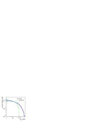
Figure 3: The differential cross-section $d\sigma/dp_{\perp,b}$ multiplied by $(m_{b}^{2}+p_{\perp,b}^{2})/p_{\perp,b}$ for the $2\to 3$ matrix element and the differential double-counting term, with $\mu_{F}=({m_{t}+m_{H^{\pm}}})/{4}$. Note the two distinct regions in the $2\to 3$ cross-section, for small and large $p_{\perp,b}$ respectively.

From the figure it is clear that for small $p_{\perp,b}$ the differential cross-section for the $2\to 3$ matrix element behaves more or less as $d\sigma/dp_{\perp,b}\propto p_{\perp,b}/m_{\perp,b}^{2}$ (similarly to the parton shower), whereas for large $p_{\perp,b}$ (where $p_{\perp,b}$ is the hard scale of the process) it behaves as $d\sigma/dp_{\perp,b}\propto 1/p_{\perp,b}^{3}$, as seen by simple dimensional analysis. This means that, as one expects on general grounds, for small $p_{\perp,b}$ the $2\to 3$ matrix element can be factorized into two parts, the $g\to b\bar{b}$ splitting and the $gb\to tH^{\pm}$ hard process (or symbolically $2\to 3=1\to 2\otimes 2\to 2$). For large $p_{\perp,b}$ on the other hand, where the outgoing $b$-quark is part of the hard process, it is not possible to factorize the process and one has to retain the complete matrix element.

These observations can now be used to identify the regions of phase space where the two approximations have their respective strength. For small $p_{\perp,b}$ we are in the collinear region where the cross-section is dominated by logarithms of the type $\left(\alpha_{s}\log(m_{\perp,b}^{2}/m_{b}^{2})\right)^{n-1}/m_{\perp,b}^{2}$ (the $2\to 3$ matrix element only contains the leading term $n=1$) and therefore resummation effects, which are included in the DGLAP evolution of the $b$-quark density, are important. For large $p_{\perp,b}$ on the other hand we are in the hard region where factorization breaks down and we have to use the $2\to 3$ matrix element.

In order to obtain the correct differential cross-sections for the accompanying $b$-quark, we need to employ a matching procedure between the $gb\to H^{\pm}t$ and $gg\to H^{\pm}tb$ processes. Just as in the case of the total cross-section the matching is done by adding the two processes and subtracting the double-counting thus introduced in the collinear region. The most basic requirements of such a procedure are that all resulting differential cross-sections must be smooth, and that the integrated cross-section must be the correct one as given by eq. (5). Also the resulting differential cross-sections should be given by the leading order process for small $p_{\perp,b}$ and by the $2\to 3$ matrix element for large $p_{\perp,b}$.

The key observation in the generalization of the matching procedure to the differential cross-section is that the leading logarithmic $b$-quark density (9) defines a differential distribution in the variables $z$ and $Q^{2}$, which together with the differential cross-section for the $2\to 2$ process and two azimuthal angles gives a complete differential definition of the double-counting term. By picking events from this distribution and subtracting them in the data analysis (e.g. histograms), we can account for the double-counting not only for the total cross-section but also differentially.

In this way, we can write down the complete expression for the double-counting term based on eqs. (3) and (9) (properly accounting for the phase-space limitations as well as the mass of the incoming $b$-quark):

$$\sigma_{\mathrm{DC}}=\int_{\tau_{\mathrm{min}}}^{1}\frac{d\tau}{\tau}\int_{\frac{1}{2}\log\tau}^{-\frac{1}{2}\log\tau}dy^{*}\frac{\pi}{\hat{s}}\int_{-1}^{1}\frac{\beta_{34}}{2}d(\cos\hat{\theta})\left|\cal M_{\mathrm{LO}}\right|^{2}\,\frac{\alpha_{s}(\mu_{R}^{2})}{2\pi}\times$$ (10)

$$\left[\int_{x_{1}}^{z_{\mathrm{max}}}dzP_{g\to q\bar{q}}(z)\int_{Q^{2}_{\mathrm{min}}}^{Q^{2}_{\mathrm{max}}}\frac{d(Q^{2})}{Q^{2}+m_{b}^{2}}\,\frac{x_{1}}{z}g(\frac{x_{1}}{z},\mu_{F}^{2})\,x_{2}g(x_{2},\mu_{F}^{2})+x_{1}\leftrightarrow x_{2}\right]$$

Here $\cal M_{\mathrm{LO}}$ is the matrix element for the leading order process (1) and the variables for the $2\to 2$ process are defined as follows: $\tau=x_{1}x_{2}$, $x_{1,2}=\sqrt{\tau}e^{\pm y^{*}}$, $\hat{s}=\tau s$, $\hat{\theta}$ is the polar angle of the $t$-quark in the CM system of the $2\to 2$ scattering, and $\beta_{34}=\hat{s}^{-1}\sqrt{(\hat{s}-m_{t}^{2}-m_{H^{\pm}}^{2})^{2}-4m_{t}^{2}m_{H^{\pm}}^{2}}$.

The integration limits are given by

$$\tau_{\mathrm{min}} =(m_{t}+m_{H^{\pm}})^{2}/s$$ (11a)

$$z_{\mathrm{max}} =\frac{Q^{2}_{\mathrm{opt}}\hat{s}}{(Q^{2}_{\mathrm{opt}}+\hat{s})(Q^{2}_{\mathrm{opt}}+m_{b}^{2})}\;,\;Q^{2}_{\mathrm{opt}}=\min\left(\sqrt{\hat{s}m_{b}^{2}},\mu_{F}^{2}\right)$$ (11b)

$$Q^{2}_{\mathrm{min}} =\textstyle\frac{1}{2}\left[\hat{s}\left(z^{-1}-1\right)-m_{b}^{2}\right]-\textstyle\frac{1}{2}\sqrt{\left[\hat{s}\left(z^{-1}-1\right)-m_{b}^{2}\right]^{2}-4\hat{s}m_{b}^{2}}$$ (11c)

$$Q^{2}_{\mathrm{max}} =\min\left\{\mu_{F}^{2},\textstyle\frac{1}{2}\left[\hat{s}\left(z^{-1}-1\right)-m_{b}^{2}\right]+\textstyle\frac{1}{2}\sqrt{\left[\hat{s}\left(z^{-1}-1\right)-m_{b}^{2}\right]^{2}-4\hat{s}m_{b}^{2}}\right\}.$$ (11d)

In deriving these limits we have identified $z$ as the ratio of the center of mass energies of the $2\to 2$ and $2\to 3$ processes, $z=\hat{s}/\hat{s}^{\prime}$. Assuming that the outgoing $b$- and $t$-quarks as well as the charged Higgs boson are on-shell, this identification of $z$ gives the following expression for the transverse momentum of the outgoing $b$-quark in the center of mass system of the two gluons:

$$p_{\perp,b}^{2}=Q^{2}-z\frac{(\hat{s}+Q^{2})(m_{b}^{2}+Q^{2})}{\hat{s}}.$$ (12)

Note that $Q^{2}=-k^{2}$, where $k$ is the 4-momentum of the $b$-quark propagator. From this the limits on $z$ and $Q^{2}$ of eq. (11) follow by considering the collinear situation when $p_{\perp,b}^{2}=0$ and taking into account that the virtuality cannot be larger than the factorization scale $\mu_{F}^{2}$. In case of the upper limit on $z$ one also has to find the optimal $Q^{2}$ value which maximizes $z$ by setting $dz/dQ^{2}=0$.

It should be noted that the renormalization scale $\mu_{R}$ in eq. (10) is the same as in the hard $2\to 2$ subprocess (1) and that the gluon density related to the $g\to b\bar{b}$ splitting is evaluated at the same factorization scale $\mu_{F}$ as the $b^{\prime}$-density and the other incoming gluon. These choices corresponds to requiring that the double-counting term approximates the $2\to 3$ matrix element for small $p_{\perp,b}$. In the Pythia parton shower the renormalization scale is given by $(1-z)Q^{2}\simeq p_{\perp,b}^{2}$ and the factorization scale by $Q^{2}$, and since the parton shower corresponds to a leading-logarithmic resummation, $\alpha_{s}$ is calculated at 1-loop. For $p_{\perp,b}\sim\mu_{F}$, the difference between the different scale choices is negligible and thus the double-counting term will approach the distribution obtained from the $2\to 2$ process with parton showers in this region, ensuring that the matched differential cross-section smoothly interpolates between the $2\to 2$ process for small $p_{\perp,b}$ and the $2\to 3$ process for large $p_{\perp,b}$.

Taking the limit $\hat{s}\to\infty$, eq. (12) also gives the relation

$$\frac{dQ^{2}}{Q^{2}+m_{b}^{2}}=\frac{dp_{\perp,b}^{2}}{p_{\perp,b}^{2}+m_{b}^{2}}$$ (13)

which explains the plateau for small $p_{\perp,b}$ seen in fig. 3 for both the double-counting term and the $2\to 3$ matrix element. The figure also illustrates the importance of the kinematic constraints in the double-counting term which otherwise would have been flat all the way up to $p_{\perp,b}=\mu_{F}$. In section 5 we will discuss how the extension of this plateau can be used to set a proper factorization scale for the $2\to 2$ process.

The differential cross-section for the double-counting term has been implemented as an external process to Pythia and will be made available for download [26] whereas the $2\to 3$ process is implemented as a regular process in Pythia from version 6.223.

4 Results of the matching procedure

In this section we present the results from a case study of our matching procedure using $m_{H^{\pm}}=250\mathrm{\;GeV}$ and $\tan\beta=30$ at LHC energies.

We use Pythia, including initial- and final-state radiation, with default settings, except that the factorization scale is set to be $\mu_{F}=(m_{t}+m_{H^{\pm}})/4$ (this choice of factorization scale will be motivated in section 5), and $\alpha_{s}$ in the hard process and the running $b$-quark mass entering the Yukawa coupling are evaluated at $m_{H^{\pm}}$ (we use a 1-loop expression for $\alpha_{s}$ and the Yukawa coupling since we are effectively dealing with a leading order process as argued in connection with eq. 5). In addition the outgoing $b$-quark in the initial state parton shower as well as in the double-counting term is put on-shell in order to facilitate a more clearcut comparison with the $2\to 3$ process, where the outgoing $b$-quark is on-shell. In a realistic case, using jet-finding algorithms, there should be no observable difference compared to having the outgoing $b$-quark off-shell in the parton shower. Finally the maximal scale for the initial state shower is set to the factorization scale and we use the CTEQ5L parton densities.

Since we are only dealing with leading order calculations the overall normalization is quite uncertain, especially given that the cross-section is proportional to the renormalized $b$-quark mass from the Yukawa coupling. Therefore, in the following we will concentrate on the shapes of the distributions. The results for differential cross-sections in a few different variables are presented in figs. 4 and 5.

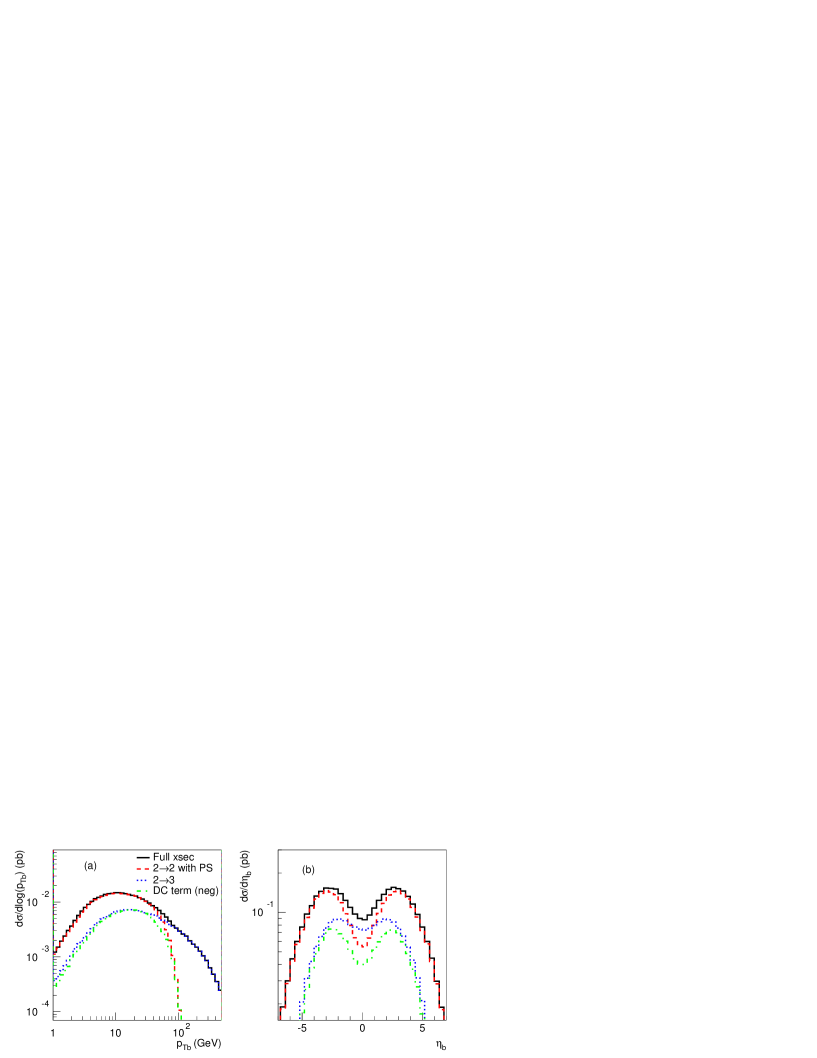
Figure 4: Differential distributions in (a) $p_{\perp,b}$ and (b) $\eta_{b}$ for the cross-section contributions ($2\to 2$ process, $2\to 3$ process and double-counting term) and the resulting matched cross-section for $\tan\beta=30$, $m_{H^{\pm}}=250\mathrm{\;GeV}$, $\mu_{F}=(m_{t}+m_{H^{\pm}})/4$. Note that the double-counting term contribution (DC) is subtracted from the sum.

First of all it is clear from fig. 4a that the matched $p_{\perp,b}$-distribution looks as expected. It follows the leading order cross-section for small $p_{\perp,b}$, where the $b$-quark is collinear with the incoming gluon, and the $2\to 3$ process for large $p_{\perp,b}$, where the matrix element should give the correct $p_{\perp,b}$ distribution. For intermediate $p_{\perp,b}\lesssim\mu_{F}$, the double-counting term interpolates smoothly between the two approximations giving an overall smooth transition between the collinear and hard regions. We also note that the transition region is quite wide ranging in this case from $\approx 10\mathrm{\;GeV}$ to $\approx 100\mathrm{\;GeV}$.

Restricting ourselves to the experimentally interesting region where $b$-quarks can be tagged, i.e. $p_{\perp,b}\gtrsim 20\mathrm{\;GeV}$ , we see that the shape of the $p_{\perp,b}$-distribution deviates substantially from the one given by the $2\to 3$ process. In fact, close to this lower limit the matched distribution is about twice as large as the $2\to 3$ process. In other words, if one only uses the $2\to 3$ process, the high-$p_{\perp,b}$ region will be strongly overestimated compared to the low-$p_{\perp,b}$ one. Similarly for $\eta_{b}$ (fig. 4b), in the experimentally interesting region $|\eta_{b}|<2.5$, the shape differs substantially both from the leading order and the $2\to 3$ processes, again illustrating that one has to use matching in order to get a reliable description of the outgoing $b$-quark.

From fig. 4a it is also clear that the method suggested in [20] for matching the LO and $2\to 3$ processes by making a cut in the $p_{\perp,b}$, using the $2\to 3$ process for events with $p_{\perp,b}>p_{\perp,\mathrm{cut}}$ and the LO process for $p_{\perp,b}<p_{\perp,\mathrm{cut}}$, rescaled such that the total cross-section is given by eq. (5), does not work in general. Such a matching procedure gives the correct cross-section behavior for large $p_{\perp,b}$ where both the leading order process and the double-counting term are negligible, but the draw-back is that the normalization is changed for small $p_{\perp,b}$ relative to large $p_{\perp,b}$ since the double-counting is only subtracted for $p_{\perp,b}<p_{\perp,\mathrm{cut}}$. In addition the kinematic constraints represented by the integration limits (11) were not taken into account leading to an underestimation of the cross-section, and it is also not guaranteed that the differential cross-sections are smooth in all kinematic variables.

In case one chooses not to tag the accompanying $b$-quark the differences between the differential distributions from the $2\to 2$ process and the matched ones are not as significant. As an example we have chosen to look at the distributions of the $b$-quark originating from the top quark decay and the hadronic $\tau$-jet originating from the charged Higgs bosons decay, which are of primary interest when studying hadronic $\tau$-decays of heavy charged Higgs bosons (see e.g. [14]).

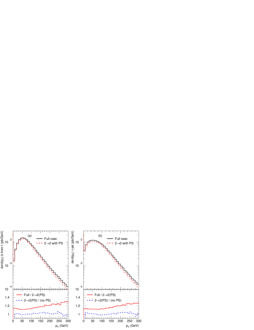
Figure 5: Transverse momentum distributions of: (a) the $b$-quark from the top decay, (b) the hadronic $\tau$-jet from $H^{\pm}\to\tau^{\pm}\nu_{\tau}$, for $\tan\beta=30$, $m_{H^{\pm}}=250\mathrm{\;GeV}$, and $\mu_{F}=(m_{t}+m_{H^{\pm}})/4$. The upper panels show the matched result (solid) compared to the $2\to 2$ process with parton showers (dashed), whereas the lower panels show the ratio of the two (solid) as well the ratio of the $2\to 2$ process with and without parton showers (dashed).

The effects of matching on these distributions are shown in fig. 5. As can be seen from fig. 5a the effects on the shape of the transverse momentum distribution of the $b$-quark from the top quark decay amounts to $10-15\%$ compared to the leading order process in the region $p_{\perp,b}\lesssim 250\mathrm{\;GeV}$. Similar results are obtained for the $\tau$-jet from the decay of the charged Higgs boson, as seen in fig. 5b. These results, except for the normalization, are not very sensitive to the choice of factorization scale. As a way to gauge the importance of these effects fig. 5 also shows the effect of turning off the partons showers on these distributions. From the figure it is clear that with the scale for the partons showers set to $\mu_{F}=(m_{t}+m_{H^{\pm}})/4$, the effects of matching are larger than the effects of the parton shower. However, if one instead sets the scale of the parton shower to be $(m_{t}+m_{H^{\pm}})$, then the parton shower has a somewhat larger impact on the shape of the distributions than the matching.

At the same time we have found that the effects of matching depend on the cuts used in defining the signal. If the cuts are chosen carefully as in [14] the differences in the shape of the distributions are diminished. As a consequence it is not possible to make a general statement about the need to including matching when the accompanying $b$-quark is not observed. Instead one has to investigate this from case to case if one wants to pin down uncertainties of the size illustrated in fig. 5.

5 Factorization scale dependence

Until now we have used what may appear to be a rather small factorization scale $\mu_{F}=(m_{t}+m_{H^{\pm}})/4$ compared to the more conventional choice of $\mu_{F}\sim\sqrt{\hat{s}}\simeq m_{t}+m_{H^{\pm}}$. Of course, in an all orders calculation the factorization scale dependence drops out, but when the perturbative series is truncated one is left with a residual scale dependence which can be quite large especially in leading order calculations as we are dealing with here. However, this formal independence on the factorization scale when going to all orders does not mean that the choice is arbitrary. On the contrary, as we have already seen, the matrix element for the $2\to 3$ process gives a clear indication of where the transition between the collinear and hard regions takes place. The important point to keep in mind is that the collinear parton density integrates over all $p_{\perp}$ of the parton up to the factorization scale. In other words, we can get a good indication of a proper choice of factorization scale for the leading order process from the $p_{\perp,b}$-distribution of the matrix element for the $2\to 3$ process shown in fig. 3.

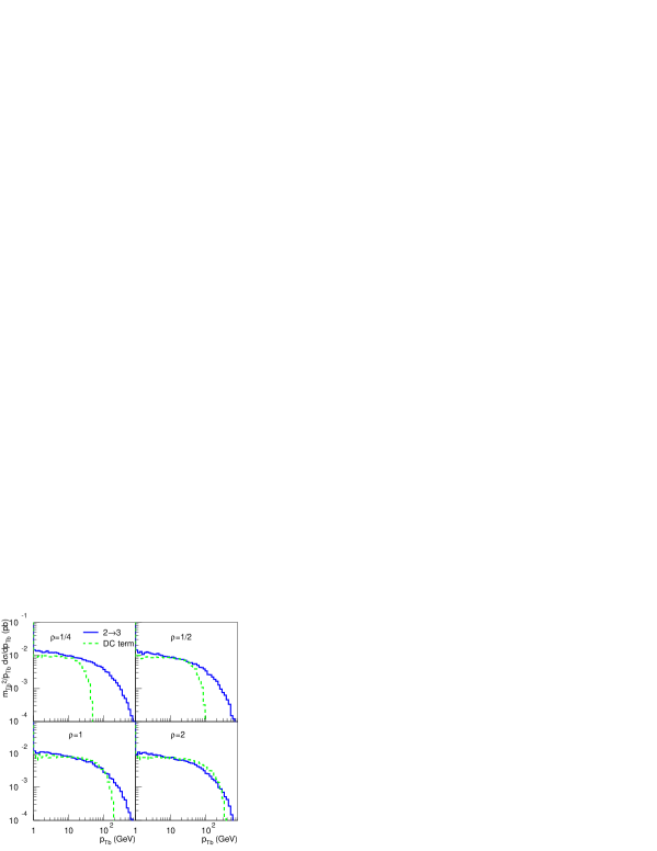
Figure 6: The differential cross-section $d\sigma/dp_{\perp,b}$ multiplied by $m_{\perp,b}^{2}/p_{\perp,b}$ for the $2\to 3$ matrix element and the double-counting term for different factorization scales parameterized by $\rho=2\mu_{F}/(m_{t}+m_{H^{\pm}})$.

In order to be able to extract a suitable factorization scale from the $p_{\perp,b}$-distribution it is instructive to compare the matrix element with the double-counting term since the latter is based on the collinear approximation. Naively one would expect the double-counting term to have a flat $p_{\perp,b}$-distribution when multiplied with $m_{\perp,b}^{2}/p_{\perp,b}$ all the way up to the factorization scale and then drop to zero. However, as is clear from fig. 3 this is not true. The difference is mainly due to the kinematic constraints and a non-constant gluon-density. Comparing the two distributions for different factorization scales, shown in fig. 6, we see that a suitable factorization scale is obtained by requiring that the plateau in the distribution for the double-counting term extends to the same $p_{\perp,b}$ as the matrix element but does not overshoot it. In this way we ensure that the size of the collinear logarithms in the $b$-quark density are not overestimated. It follows that the factorization scale should be $\mu_{F}\approx(m_{t}+m_{H^{\pm}})/4$. We also see that the “standard” choice $\mu_{F}=m_{t}+m_{H^{\pm}}$ leads to a large overestimation of the collinear logs.

The $p_{\perp,b}$-distribution was also used to find an appropriate factorization scale in [6] and [7] when studying the next-to-leading order corrections to the $gb\to tH^{-}$ process. In [6] the factorization scale was chosen such that the integral over transverse momentum of the asymptotic form of the differential cross-section, $\left.d\sigma/dp_{\perp,b}\right|_{\rm asympt}=S\,p_{\perp,b}/m_{\perp,b}^{2}$, gives the same total cross-section as the $2\to 3$ process, whereas in [7] one compared the asymptotic behavior of the transverse momentum distribution with the extent of the plateau in the $2\to 3$ process. Based on these arguments they suggest that a suitable factorization scale is $\mu_{F}\approx(m_{t}+m_{H^{\pm}})/6$ and $\mu_{F}\approx(m_{t}+m_{H^{\pm}})/5$ respectively which is very similar to what we find.

The question of finding an appropriate factorization scale is not particular to charged Higgs boson production. In neutral Higgs boson production in association with bottom quarks one faces a similar situation where the question of whether to treat the incoming $b$-quarks as partons or not is also important and one can use similar arguments for the appropriate factorization scale to be used. In [27, 28] the transverse momentum distribution of $b$-quarks in the process $gg\to b\bar{b}h$ was compared to the factorized expectation $d\sigma/dp_{\perp,b}\propto p_{\perp,b}/m_{\perp,b}^{2}$. Using the argument that these two distributions should approximately agree up to the factorization scale, it was found that a factorization scale of order of $m_{h}/10$ is more proper than the usual $\mu_{F}={\cal O}(m_{h})$. Based on the same argument, a similar conclusion was also drawn in case of charged Higgs boson pair-production in association with bottom quarks [29]. In another approach [30, 31] one instead looked at the distribution in Mandelstam-$t$ for the processes $bg\to hb$ and $b\bar{b}\to gh$ scaled with the Higgs boson mass, $-td\sigma/dt(\sqrt{-t}/m_{h})$. Using these arguments the authors argue that a small factorization scale $\mu_{F}\approx m_{h}/4$ is preferable. Finally, comparing the NNLO calculation of $b\bar{b}\to h$ with the LO and NLO ones one [32] finds that both the scale dependence and higher order corrections are small when $(\mu_{R},\mu_{F})\sim(m_{h},m_{h}/4)$.

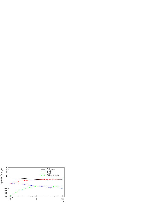
Figure 7: Integrated cross-sections at $m_{H^{\pm}}=250\mathrm{\;GeV}$ and $\tan\beta=30$ as a function of the factorization scale parametrized by $\rho=2\mu_{F}/(m_{t}+m_{H^{\pm}})$.

Given that the arguments for choosing the factorization scale to be $\mu_{F}=(m_{t}+m_{H^{\pm}})/4$ are not very precise we have studied to what extent the results of the matching procedure changes when varying the factorization scale (in most cases by varying it by a factor two up or down). In order not to confuse the picture we have kept the renormalization scale in $\alpha_{s}$ and the running $b$-quark mass fixed.

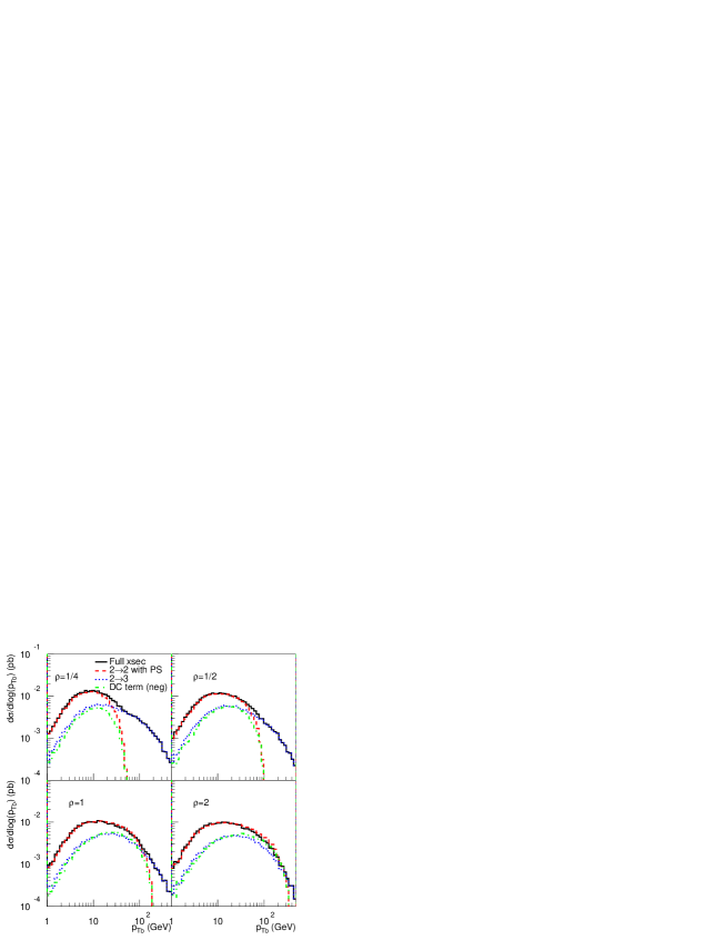
Figure 8: The different components of the differential cross-section in $p_{\perp,b}$ for different choices of the factorization scale parametrized by $\rho=\frac{2\mu_{F}}{(m_{t}+m_{H^{\pm}})}=1/4,\,1/2,\,1,\,2$.

We start out by considering the factorization scale dependence of the matched total cross-section. Parameterizing the factorization scale using the parameter $\rho$:

$$\mu_{F}=\rho\,\frac{m_{t}+m_{H^{\pm}}}{2}$$ (14)

we get the result shown in fig. 7. Comparing with the scale dependence of the different components ($2\to 2$, $2\to 3$ and double-counting) which are also displayed we see that the scale dependence is substantially reduced after matching. For example, varying the factorization scale a factor 2 up or down from $\rho=0.5$ the cross-section changes with less than 10%. This reduced factorization scale dependence is expected since we are including parts of the NLO corrections (more specifically the real corrections from gluon splitting into $b\bar{b}$-pairs in the initial state) to the leading order process. The same reduction of the scale dependence has also been seen in neutral Higgs boson production via $b$-quark fusion [30]. In addition we see that at $\rho\gtrsim 1$ the double-counting term becomes larger than the $2\to 3$ process. In view of the fact that the double-counting term is included in order to cancel the component of the $2\to 3$ process that is already included in the leading order process, this marks a breakdown in the procedure, indicating that the factorization scale is chosen too large.

Next we consider the matching procedure itself. As can be seen from fig. 8, showing the $p_{\perp}$-distribution of the $b$-quark, the matching procedure still fulfills the requirements outlined in section 3 for other factorization scales but the relative importance of the different contributions varies. However, for the case $\rho\gtrsim 1$, the double-counting term is overshooting the $2\to 3$ process in the region $p_{\perp,b}\lesssim\mu_{F}$, again indicating that this choice of factorization scale is too large.

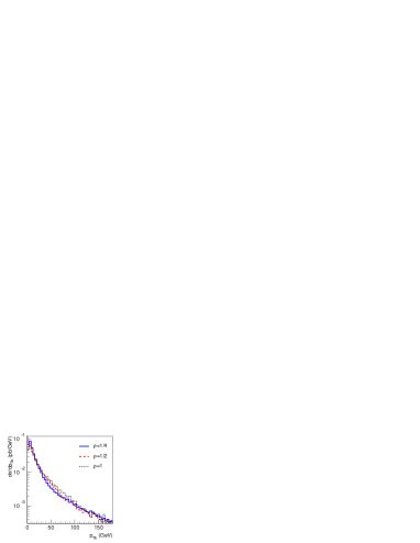
Figure 9: Matched $p_{\perp,b}$-differential cross-sections for different choices of the factorization scale, $\rho=\frac{2\mu_{F}}{(m_{t}+m_{H^{\pm}})}=1/4,\,1/2,\,1$.

Finally fig. 9 shows the relative stability of the matched $p_{\perp,b}$-distribution when varying the factorization scale up or down with a factor 2 from our preferred value. From the figure we see that the residual factorization scale uncertainty is typically small and at most $\sim 20\%$ (in the region $p_{\perp,b}\sim(m_{t}+m_{H^{\pm}})/5$). This should be compared with the difference between the matched distribution and the one from the $2\to 3$ matrix element which amounts to a factor $\sim 2$ at $p_{\perp,b}\sim 20$ GeV.

6 Conclusions and Outlook

In this paper we have presented a new method for matching the $gb\to H^{\pm}t$ and $gg\to H^{\pm}tb$ processes in Monte Carlo event generators such as Pythia and Herwig. By matching the two processes at hand in a proper way we can combine their respective virtues. On the one hand, the $gb\to H^{\pm}t$ (or $2\to 2$) process includes a resummation of potentially large logarithms of the type $\alpha_{s}\log(\mu_{F}/m_{b})$ which arise from the collinear region of phase space where the transverse momentum of the accompanying $b$-quark $p_{\perp,b}$ is small. On the other hand, the $gg\to H^{\pm}tb$ (or $2\to 3$) processes contains the exact kinematics of the accompanying $b$-quark which is important in the hard region where $p_{\perp,b}$ is large.

The matching is done by adding the two different approximations and subtracting the common part which otherwise would be double-counted. In other words the double-counting term is given by the collinear approximation of the $gg\to H^{\pm}tb$ process. By viewing the double-counting term as a differential distribution in the kinematic variables of the $2\to 3$ process, it can be used to generate events in the same way as any other process, including parton showers and hadronization. These events are then subtracted from the sum of the events generated from the $gb\to H^{\pm}t$ and $gg\to H^{\pm}tb$ processes.

This matching procedure leads to a smooth transition between the collinear region of phase space, where the $2\to 2$ process dominates, and the hard region where the $2\to 3$ process dominates. Looking at the $p_{\perp,b}$-distribution the difference between the matched cross-section and the $2\to 3$ process can be as large as a factor $\sim 2$ in regions of experimental interest ($p_{\perp,b}\gtrsim 20$ GeV). Likewise, the pseudorapidity distribution of the accompanying $b$-quark differs significantly in shape from both the $2\to 2$ and the $2\to 3$ process in the central region. When looking at the distributions of the decay products of the $t$-quark and the charged Higgs boson the differences are smaller, typically $\sim 10\%$ in experimentally interesting regions of phase space which is similar to the effects of parton showers. At the same time, the differences turn out to be sensitive to the cuts used to define the signal and by carefully choosing the cuts, as in [14], the effects can be made negligible.

Not only does the matching procedure give a better description of charged Higgs boson production, in addition it also gives a reduced factorization scale dependence. The sum of the different contributions to the total cross-section has a much smaller factorization scale dependence than the individual parts. Looking at the $p_{\perp,b}$-distribution from the $gg\to H^{\pm}tb$ matrix element and comparing to the double-counting term we also get strong arguments for choosing a factorization scale $\mu_{F}=(m_{t}+m_{H^{\pm}})/4$ which is substantially smaller than the “standard choice” $\mu_{F}\sim\sqrt{\hat{s}}\simeq(m_{t}+m_{H^{\pm}})$. Being conservative we estimate the remaining factorization scale dependence by varying the factorization scale with a factor two. Doing this we find that the total cross-section varies with about $\pm 10\%$ and that the height of the $p_{\perp,b}$-distribution is also quite stable, varying at most about $\pm 20\%$.

The method that we have presented in this paper is not restricted to charged Higgs boson production. It can also be applied in other processes where one has incoming $b$-quarks. The simplest example is $gb\to W^{\pm}t$-production, but it can also be extended to include processes with two incoming $b$-quarks, such as Higgs boson production in association with $b$-quarks. It would also be interesting to extend the method to also include the remaining NLO corrections to get a NLO normalization of the total cross-section as in the MC@NLO method.

- [1] [LEP Higgs Working Group for Higgs boson searches Collaboration], arXiv:hep-ex/0107031.
- [2] F. Abe et al. [CDF Collaboration], Phys. Rev. Lett. 79 (1997) 357 [arXiv:hep-ex/9704003]. T. Affolder et al. [CDF Collaboration], Phys. Rev. D 62 (2000) 012004 [arXiv:hep-ex/9912013].
- [3] B. Abbott et al. [D0 Collaboration], Phys. Rev. Lett. 82 (1999) 4975 [arXiv:hep-ex/9902028]. V. M. Abazov et al. [D0 Collaboration], Phys. Rev. Lett. 88 (2002) 151803 [arXiv:hep-ex/0102039].
- [4] D. P. Roy, Mod. Phys. Lett. A 19 (2004) 1813 [arXiv:hep-ph/0406102].
- [5] S. h. Zhu, Phys. Rev. D 67 (2003) 075006 [arXiv:hep-ph/0112109].
- [6] T. Plehn, Phys. Rev. D 67 (2003) 014018 [arXiv:hep-ph/0206121].
- [7] E. L. Berger, T. Han, J. Jiang and T. Plehn, arXiv:hep-ph/0312286.
- [8] T. Sjöstrand et al. Comput. Phys. Commun. 135 (2001) 238 [arXiv:hep-ph/0010017].
- [9] G. Corcella et al., JHEP 0101 (2001) 010, [arXiv:hep-ph/0011363].
- [10] S. Frixione and B. R. Webber, JHEP 0206, 029 (2002) [arXiv:hep-ph/0204244].
- [11] F. Borzumati, J. L. Kneur and N. Polonsky, Phys. Rev. D 60 (1999) 115011 [arXiv:hep-ph/9905443].
- [12] R. M. Barnett, H. E. Haber and D. E. Soper, Nucl. Phys. B 306 (1988) 697.
- [13] F. I. Olness and W. K. Tung, Nucl. Phys. B 308 (1988) 813.
- [14] K. A. Assamagan and Y. Coadou, Acta Phys. Polon. B 33 (2002) 707.
- [15] K. A. Assamagan, Y. Coadou and A. Deandrea, Eur. Phys. J. directC 4 (2002) 9 [arXiv:hep-ph/0203121].
- [16] R. Kinnunen, “Study of Heavy Charged Higgs in with in CMS”, CMS NOTE 2000/045 (available from http://cmsdoc.cern.ch/doc/notes/docs/NOTE2000_045)
- [17] D. P. Roy, Phys. Lett. B 459 (1999) 607 [arXiv:hep-ph/9905542].
- [18] D. J. Miller, S. Moretti, D. P. Roy and W. J. Stirling, Phys. Rev. D 61 (2000) 055011 [arXiv:hep-ph/9906230].
- [19] K. A. Assamagan and N. Gollub, arXiv:hep-ph/0406013.
- [20] A. Belyaev, D. Garcia, J. Guasch and J. Sola, JHEP 0206 (2002) 059 [arXiv:hep-ph/0203031].
- [21] H. L. Lai et al. [CTEQ Collaboration], Eur. Phys. J. C 12 (2000) 375 [arXiv:hep-ph/9903282].
- [22] J. Alwall, C. Biscarat, S. Moretti, J. Rathsman and A. Sopczak, Eur. Phys. J. directC 1 (2004) 005 [arXiv:hep-ph/0312301].
- [23] D. Dicus, T. Stelzer, Z. Sullivan and S. Willenbrock, Phys. Rev. D 59 (1999) 094016 [arXiv:hep-ph/9811492].
- [24] S. Frixione, P. Nason and B. R. Webber, JHEP 0308, 007 (2003) [arXiv:hep-ph/0305252].
- [25] R. Vogt and S. J. Brodsky, Nucl. Phys. B 438, 261 (1995) [arXiv:hep-ph/9405236].
- [26] The Fortran code for the double-counting term, implemented as an external process to Pythia will be available at http://www3.tsl.uu.se/thep/MC/pytbh/, including a manual in preparation.
- [27] D. L. Rainwater, M. Spira and D. Zeppenfeld, arXiv:hep-ph/0203187.
- [28] M. Spira, arXiv:hep-ph/0211145.
- [29] S. Moretti and J. Rathsman, Eur. Phys. J. C 33 (2004) 41 [arXiv:hep-ph/0308215].
- [30] F. Maltoni, Z. Sullivan and S. Willenbrock, Phys. Rev. D 67 (2003) 093005 [arXiv:hep-ph/0301033].
- [31] E. Boos and T. Plehn, Phys. Rev. D 69 (2004) 094005 [arXiv:hep-ph/0304034].
- [32] R. V. Harlander and W. B. Kilgore, Phys. Rev. D 68 (2003) 013001 [arXiv:hep-ph/0304035].