Transport coefficients and the 2PI effective action in the large $N$ limit

Abstract

We discuss the computation of transport coefficients in large $N_{f}$ QCD and the $O(N)$ model for massive particles. The calculation is organized using the $1/N$ expansion of the 2PI effective action to next-to-leading order. For the gauge theory, we verify gauge fixing independence and consistency with the Ward identity. In the gauge theory, we find a nontrivial dependence on the fermion mass.

1 Motivation

In understanding the evolution of quantum fields out of equilibrium, thermalization plays an important role. For long enough times, the dynamics of a typical system can be characterized by transport coefficients, as they control the relaxation of a system towards equilibrium. For example, in heavy ion collisions, the presence of an appreciable shear viscosity would modify the ideal hydrodynamical description[1] of the aftermath of the collision.[2, 3]

The nonequilibrium evolution of quantum fields and the subsequent thermalization have been studied using various approximations: mean-field dynamics (such as Hartree or leading-order large $N$ approximations), inhomogeneous mean-field theory, the classical approximation, kinetic theory, dynamics based on truncations of the 2PI or 2PPI effective action, etc. It is clear that any scheme aimed at describing the long-time behavior should, among other things, describe correctly the approach to equilibrium of a typical system. One requirement for an approximation scheme is therefore to yield sensible results for transport coefficients. While it is clear that some approaches (mean-field theory, classical approximation) do not give the correct long-time quantum behavior, for others this might be more involved.

One approach to the dynamics of quantum fields far from equilibrium that has been successful in the past few years[4]^-[15] employs the 2PI effective action.[16] It is therefore interesting to see whether the 2PI framework gives a reliable description of transport coefficients, in the limit where a semi-analytical computation can be carried out, i.e. in a weak coupling or a large $N$ expansion. Below we review how transport coefficients can be computed using the 2PI effective action as an organizational tool.[17] We discuss explicitly two theories in the large $N$ limit: the shear viscosity in the $O(N)$ model[18] and the electrical conductivity and shear viscosity in large $N_{f}$ QCD with massive fermions.[19]

2 2PI effective action

The 2PI effective action offers an approach to deal with the infinite hierarchy of correlation functions in field theory, based on a variational principle for one- and two-point functions. For a bosonic field, with vanishing mean field $\langle\phi\rangle=0$, the effective action is written as[16]

$$\Gamma[G]=\frac{i}{2}{\mathrm{Tr}}\ln G^{-1}+\frac{i}{2}{\mathrm{Tr}}\,G_{0}^{-1}(G-G_{0})+\Gamma_{2}[G],$$ (1)

where $G_{0}^{-1}$ is the free inverse propagator. $\Gamma_{2}[G]$ contains all two-particle irreducible diagrams without external legs. For fermionic fields the $\frac{1}{2}$’s are replaced by $-1$’s. Although the attention is usually focused on the (one- and) two-point functions, the 2PI effective action is formulated as a generating functional with external sources, similar to the 1PI effective action, and therefore higher order $n$-point functions are accessible as well. In particular, there is a four-point vertex function obeying a Bethe-Salpeter equation, which in momentum space reads

$$\Gamma^{(4)}(P,K)=\Lambda(P,K)+\frac{1}{2}\int_{R}\Lambda(P,R)G^{2}(R)\Gamma^{(4)}(R,K).$$ (2)

This equation sums ladder diagrams with a kernel $\Lambda$ obtained from the second derivative of $\Gamma_{2}[G]$. It plays therefore a crucial role in the computation of transport coefficients[17] in the case that these are dominated by ladder diagrams, such as in scalar[20, 18] and large $N_{f}$ gauge theories[19] to leading order and in weakly coupled gauge theories to leading logarithmic order.[21]

We now apply this to two theories in the large $N$ limit: the $O(N)$ model and large $N_{f}$ QCD. We consider the shear viscosity in the $O(N)$ model with massive particles both at weak coupling as well as in the large $N$ limit. For a weakly-coupled single-component scalar field the shear viscosity was computed some time ago by Jeon.[20] In large $N_{f}$ QCD, we present the first diagrammatic calculation of the electrical conductivity and shear viscosity for massive fermions. For massless fermions, these transport coefficients were computed before by Moore[22] using kinetic theory.

                 

Figure 1: 2PI contribution to the effective action at LO and NLO in the large $N$ limit in the $O(N)$ model (left) and at NLO in large $N_{f}$ QCD (right). The dashed line in the $O(N)$ model sums the chain of bubbles, see Fig. 2.

The starting point is the 2PI contribution to the effective action in the $1/N$ expansion, shown in Fig. 1. In the $O(N)$ model there is a LO and a NLO contribution.[7, 9] In large $N_{f}$ QCD there is only a contribution at NLO. The chain of bubbles in the $O(N)$ model is indicated with the dashed line (see Fig. 2). In this formulation the scalar and gauge theory are conveniently similar. We emphasize that all results below are generated from the graphs in Fig. 1, indicating the power of the 2PI formalism.

Figure 2: Auxiliary correlator in the $O(N)$ model, summing the chain of bubbles.

Extremizing the effective action yields the Schwinger-Dyson equations for the two-point functions. For the scalar case we find

$$G^{-1}=G_{0}^{-1}-\Sigma,\;\;\;\;\;\;\;\;D^{-1}=D_{0}^{-1}-\Pi,$$ (3)

where $G$ is the scalar and $D$ the auxiliary correlator. For the gauge theory

$$S^{-1}=S_{0}^{-1}-\Sigma,\;\;\;\;\;\;\;\;D^{-1}=D_{0}^{-1}-\Pi,$$ (4)

with $S$ the fermion and $D$ the gauge field propagator. The self energies, depending on full propagators, are shown in Fig. 3.

              

Figure 3: Self energies at LO and NLO in the large $N$ limit in the $O(N)$ model (left) and at NLO in large $N_{f}$ QCD (right).

In the computation of transport coefficients, it is crucial to use dressed propagators for two reasons: to screen the so-called pinching poles,[23, 20] reflecting the dependence on the finite lifetime of quasiparticles due to collisions in the plasma, and to screen the divergences due to the exchange of offshell gauge bosons[24] (this only in the gauge theory).

Differentiating the self energies yields the rungs that appear in the Bethe-Salpeter equation. We find that some rungs contribute to the transport coefficients at leading order, whereas other rungs are subleading and can be neglected. When considering the Bethe-Salpeter equation for other purposes (e.g. for renormalization[25, 26, 27]) we expect that all rungs that follow from the effective action might have to be considered.

            

Figure 4: Kernels at LO and NLO in the large $N$ limit in the $O(N)$ model (left) and at NLO in large $N_{f}$ QCD (right).

In order to distinguish leading from subleading rungs, we need to discuss power counting. In the large $N$ expansion, this is fairly straightforward. Positive powers of $N$ arise from two sources: closed loops of scalar or fermionic lines and scalar or fermionic propagators suffering from pinching poles (pinching poles are screened by the scalar or fermionic thermal width $\Gamma_{\mathbf{p}}$ and result in contributions $\sim 1/\Gamma_{\mathbf{p}}\sim N$). Negative powers of $N$ arise from the coupling constants, which are taken to scale as $1/N$ as is usually done in $1/N$ expansions. As a result we find the rungs given in Fig. 4. In the $O(N)$ model, the first point-like rung does not contribute for kinematical reasons. In large $N_{f}$ QCD, the contribution from generic onshell gauge fields is subleading: the gauge field propagator appears therefore only in rungs and there is no need to consider the thermal width of onshell gauge bosons. The thermal width of an onshell fermion determined by the self energy in Fig. 3 is ill-defined.[23, 28] However, the problematic part cancels against part of the contribution from the line diagram in the kernel.[23, 21] Finally, we note that the two box diagrams in large $N_{f}$ QCD differ only in the orientation of the fermion lines; this ensures that Furry’s theorem is satisfied.

3 Summation of ladders

To sum the ladder series, we use the technique recently presented by Valle Basagoiti,[21] employing the Matsubara formalism and an effective three-point vertex ${\mathcal{D}}$. In terms of this vertex, the integral equations are shown in Figs. 5, 6.

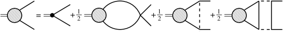
Figure 5: Integral equation for the effective vertex in the $O(N)$ model. The first closed loop on the RHS does not contribute.

Note that the propagators in these diagrams are still dressed. We consider these equations in the kinematical configuration special for transport coefficients: the momentum entering on the left is $Q=(q^{0}\to 0,{\mathbf{0}})$, while the momentum entering and leaving on the right is $P=(\omega_{\mathbf{p}},{\mathbf{p}})$, where $\omega_{\mathbf{p}}=\sqrt{{\mathbf{p}}^{2}+m^{2}}$ with $m$ the scalar or fermion mass. Transport coefficients are then extracted from the correlator obtained by closing the lines with an insertion of the appropriate current, indicated with the small black dot.[21, 17, 18, 19]

Figure 6: Integral equation for the effective vertex in large $N_{f}$ QCD. In the case of the electrical conductivity, the last two contributions cancel.

The basic quantity we use to solve the integral equations is the ratio of the effective vertex ${\mathcal{D}}(p)$ and the thermal width $\Gamma_{\mathbf{p}}$. For the shear viscosity we define

$$\chi(p)=\frac{p^{2}}{\omega_{\mathbf{p}}}\frac{{\mathcal{D}}(p)}{\Gamma_{\mathbf{p}}}\times\begin{cases}1&O(N)\\ C_{F}/T_{F}&\text{large $N_{f}$ QCD}\end{cases}$$ (5)

with $C_{F}=(N_{c}^{2}-1)/2N_{c}$, $T_{F}=1/2$. Introducing the color factors in this way removes all color factors from the integral equation. The shear viscosity in large $N_{f}$ QCD then follows from a one-dimensional integral,

$$\eta=-\frac{d_{F}T_{F}}{C_{F}}\frac{2N_{f}}{15\pi^{2}}\int_{0}^{\infty}dp\,\frac{p^{4}}{\omega_{\mathbf{p}}}n_{F}^{\prime}(\omega_{\mathbf{p}})\chi(p)$$ (6)

with $d_{F}=N_{c}$. In terms of $\chi$ the integral equations read compactly as

$${\mathcal{F}}(p)\chi(p)={\mathcal{S}}(p)+\int_{0}^{\infty}dr\,{\mathcal{H}}(p,r)\chi(r),$$ (7)

where ${\mathcal{F}}(p)\propto\Gamma_{\mathbf{p}}$, ${\mathcal{S}}(p)$ is determined by the bare vertex, and ${\mathcal{H}}={\mathcal{H}}_{\rm line}+{\mathcal{H}}_{\rm box}$ is determined by the rungs. Since ${\mathcal{H}}(p,r)={\mathcal{H}}(r,p)$, the integral equations follow as the extremum condition from the functional

$$Q[\chi]=\int_{0}^{\infty}dp\left[{\mathcal{S}}(p)\chi(p)-\frac{1}{2}{\mathcal{F}}(p)\chi^{2}(p)+\frac{1}{2}\int_{0}^{\infty}dr\,{\mathcal{H}}(p,r)\chi(r)\chi(p)\right],$$ (8)

which allows for a variational treatment. The value of $Q$ at the extremum is immediately proportional to the transport coefficient.

4 Gauge fixing and Ward identity

In applications of 2PI effective action techniques to gauge theories, gauge fixing and Ward identities have to be considered.[29, 30, 31] It is therefore interesting to see where gauge fixing parameters appear and why they drop out in the calculation. We use the generalized Coulomb gauge such that the gauge field propagator,

$$D^{\mu\nu}=\Delta_{T}P^{\mu\nu}_{T}+\Delta_{L}g^{\mu 0}g^{\nu 0}+\xi\frac{P^{\mu}P^{\nu}}{p^{4}},$$ (9)

consists of a transverse, a longitudinal, and a gauge fixing piece. The gauge fixing parameter $\xi$ appears in three places:

1. thermal width. The imaginary part of the fermionic self energy is proportional to the discontinuity (spectral density) of the gauge boson propagator, i.e. to $\rho_{T}$, $\rho_{L}$. Since the gauge fixing part has no discontinuity, $\xi$ drops out.

2. line diagram. In the kinematical limit we consider also this contribution is proportional to the discontinuity of the gauge boson propagator and $\xi$ drops out.

3. box diagram. In the kinematical limit we consider all fermion lines are onshell and $\xi$ drops out exactly.

One can also verify that the effective vertex in Fig. 6 and the fermion self energy are related via the Ward identity, again in the kinematical limit we consider. The analysis in this case is in fact easier than for the weakly coupled case,[32] since the contribution to the thermal width arising from soft fermions in the latter is now subleading in the large $N_{f}$ expansion.[19]

When extending this approach to dynamics far from equilibrium it is necessary to include contributions that could be dropped in the leading order analysis of transport coefficients presented here. The gauge fixing dependence that will be present in that case should be suppressed for sufficiently large $N_{f}$.

5 Variational solution

The integral equations are in general too complicated to be solved analytically. In the scalar case however, we found an approximate but surprisingly accurate solution for zero mass and vanishing coupling in the limit of ultrahard momentum $p\gg T$. We find

$$\lim_{p\to\infty}\chi(p)=6912\pi\frac{N^{2}}{N+2}\frac{1}{\lambda^{2}}\frac{p^{2}}{T^{2}}.$$ (10)

Using this result yields for the shear viscosity in the weakly coupled $O(N)$ model,

$$\eta_{\infty}=\frac{27648\zeta(5)}{\pi}\frac{N^{3}}{N+2}\frac{T^{3}}{\lambda^{2}}\approx 3041.9\frac{3N^{3}}{N+2}\frac{T^{3}}{\lambda^{2}}.$$ (11)

In order to obtain the full $N$ dependence and not just the leading order behavior $\sim N^{2}$ in the large $N$ limit, we used the three-loop expansion of the 2PI effective action in the $O(N)$ model.[18] The result for the numerical prefactor is very close to the full results obtained numerically by Jeon[20] (3040) and Arnold, Moore and Yaffe[33] (3033.5) for $N=1$.

For arbitrary values of the mass and coupling constant (limited by the presence of the Landau pole), we solve the integral equations variationally. The function $\chi$ is expanded in a set of trial functions and the remaining integrals (a one-dimensional integral for ${\mathcal{S}}$, three-dimensional integrals for ${\mathcal{F}}$ and ${\mathcal{H}}_{\rm line}$, and a four-dimensional integral for ${\mathcal{H}}_{\rm box}$) are performed numerically. We found that a set of four trial functions suffices.

The shear viscosity in the $O(N)$ model, normalized with the analytical result (11) in the large $N$ limit, is shown in Fig. 7 as a function of renormalized mass at zero temperature for various values of the running coupling constant (the result is renormalization group independent). We find that the shear viscosity increases monotonically with increasing mass. This behavior was also found by Jeon[20] for $N=1$. Interestingly, we find surprisingly little dependence (apart from that contained in $\eta_{\infty}$) on the coupling constant, for all values allowed by the Landau pole.

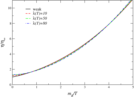
Figure 7: Shear viscosity in the $O(N)$ model vs. the renormalized mass at zero temperature for various values of the coupling constant $\lambda(\mu=T)$.

For large $N_{f}$ QCD the shear viscosity is shown as a function of fermion mass in Fig. 8, again for several values of the effective coupling constant $g_{\rm eff}$ ($g^{2}_{\rm eff}=T_{F}g^{2}N_{f}$). The viscosity is normalized with $\eta_{0}=d_{F}/(T_{F}C_{F})\times T^{3}/g^{4}$. In this case we observe a nontrivial dependence on the mass. After a slight increase, we find that the viscosity decreases with increasing mass. This behavior is caused by longitudinal gauge bosons below the lightcone. In the limit of very large mass it can be shown[34] that the viscosity goes to zero. We also find a much stronger dependence on the coupling constant, compared to the scalar theory.

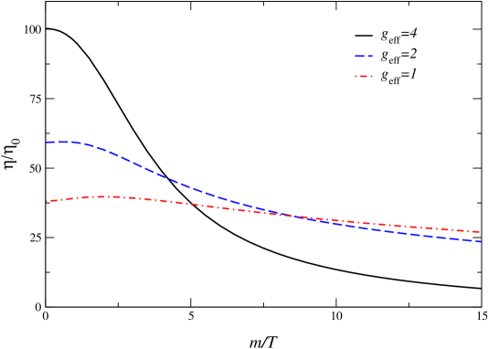
Figure 8: Shear viscosity in large $N_{f}$ QCD vs. the fermion mass for various values of the effective coupling constant $g_{\rm eff}(\mu=\pi\exp^{-\gamma_{E}}T)$.

6 Conclusion

The diagrammatic calculation of transport coefficients in the $O(N)$ model and large $N_{f}$ QCD is well organized when the 2PI effective action is used: all necessary summations are generated by the few diagrams in Fig. 1. In the scalar theory the shear viscosity increases monotonically with mass and has a dominant $1/\lambda^{2}$ dependence on the coupling constant. In the gauge theory, on the other hand, the dependence on the coupling constant and the fermion mass is highly nontrivial, due to longitudinal gauge bosons below the lightcone.

We emphasize that understanding transport coefficients diagrammatically provides necessary insight in the dynamics of quantum fields out of equilibrium. Our results provide further support for the applicability of truncations of the 2PI effective action to nonequilibrium QFT.

References

- [1] See e.g. P. F. Kolb and U. Heinz, in Hwa, R.C. (ed.) et al.: Quark gluon plasma 3, pp. 634-714 [nucl-th/0305084].
- [2] D. Teaney, Phys. Rev. C 68 (2003) 034913.
- [3] A. Muronga and D. H. Rischke, nucl-th/0407114.
- [4] J. Berges and J. Cox, Phys. Lett. B 517, 369 (2001).
- [5] B. Mihaila, F. Cooper and J. F. Dawson, Phys. Rev. D 63, 096003 (2001); ibid. 67 (2003) 051901; ibid. 67 (2003) 056003.
- [6] G. Aarts and J. Berges, Phys. Rev. D 64, 105010 (2001).
- [7] J. Berges, Nucl. Phys. A 699, 847 (2002).
- [8] G. Aarts and J. Berges, Phys. Rev. Lett. 88, 041603 (2002).
- [9] G. Aarts, D. Ahrensmeier, R. Baier, J. Berges and J. Serreau, Phys. Rev. D 66, 045008 (2002).
- [10] J. Berges and J. Serreau, Phys. Rev. Lett. 91 (2003) 111601.
- [11] J. Berges, S. Borsányi and J. Serreau, Nucl. Phys. B 660 (2003) 51.
- [12] B. Mihaila, Phys. Rev. D 68, 036002 (2003).
- [13] S. Juchem, W. Cassing and C. Greiner, Phys. Rev. D 69 (2004) 025006; nucl-th/0401046.
- [14] D. J. Bedingham, Phys. Rev. D 69, 105013 (2004).
- [15] T. Ikeda, Phys. Rev. D 69, 105018 (2004).
- [16] J. M. Cornwall, R. Jackiw and E. Tomboulis, Phys. Rev. D 10 (1974) 2428.
- [17] G. Aarts and J. M. Martínez Resco, Phys. Rev. D 68 (2003) 085009.
- [18] G. Aarts and J. M. Martínez Resco, JHEP 0402, 061 (2004).
- [19] G. Aarts and J. M. Martínez Resco, in preparation.
- [20] S. Jeon, Phys. Rev. D 52, 3591 (1995).
- [21] M. A. Valle Basagoiti, Phys. Rev. D 66, 045005 (2002).
- [22] G. D. Moore, JHEP 0105, 039 (2001).
- [23] V. V. Lebedev and A. V. Smilga, Physica A 181, 187 (1992).
- [24] G. Baym, H. Monien, C. J. Pethick and D. G. Ravenhall, Phys. Rev. Lett. 64 (1990) 1867.
- [25] H. van Hees and J. Knoll, Phys. Rev. D 65, 025010 (2002); ibid. 105005 (2002).
- [26] J. P. Blaizot, E. Iancu and U. Reinosa, Phys. Lett. B 568 (2003) 160; Nucl. Phys. A 736, 149 (2004).
- [27] F. Cooper, B. Mihaila and J. F. Dawson, hep-ph/0407119.
- [28] J. P. Blaizot and E. Iancu, Phys. Rev. D 55, 973 (1997).
- [29] A. Arrizabalaga and J. Smit, Phys. Rev. D 66, 065014 (2002).
- [30] E. Mottola, in Proceedings of SEWM2002, Heidelberg, Germany, 2-5 Oct 2002 [hep-ph/0304279].
- [31] M. E. Carrington, G. Kunstatter and H. Zaraket, hep-ph/0309084.
- [32] G. Aarts and J. M. Martínez Resco, JHEP 0211, 022 (2002).
- [33] P. Arnold, G. D. Moore and L. G. Yaffe, JHEP 0011, 001 (2000).
- [34] G. D. Moore, private communication.
- [35] P. Kovtun, D. T. Son and A. O. Starinets, JHEP 0310 (2003) 064.