Extraction of the charged pion polarizabilities from radiative charged pion photoproduction in Heavy Baryon Chiral Perturbation Theory

Abstract

We analyze the amplitude of radiative charged pion photoproduction within the framework of heavy baryon chiral perturbation theory (HBChPT) and discuss the best experimental setup for the extraction of the charged pion polarizabilities from the differential cross section. We find that the contributions from two unknown low energy constants(LECs) in the $\pi N$ chiral Lagrangian at order $p^{3}$ are comparable with the contributions of the charged pion polarizabilities. As a result, it is necessary to take these two LECs’ effects into account. Furthermore, we discuss the applicability of the extrapolation method and conclude that this method is applicable only if the polarization vector of the incoming photon is perpendicular to the scattering plane in the center of mass frame of the final $\gamma-\pi$ system.

I Introduction

Electric ($\alpha$) and magnetic ($\beta$) polarizabilities characterize the global responses of a composite system to external electric and magnetic fields. They provide precious information about the inner structure of the composite system. Since the pion is the simplest composite system bound by the strong interaction, its polarizabilities are fundamental benchmark of QCD in the realm of confinement, and an accurate determination of the charged pion polarizabilities is highly desirable. The charged pion polarizabilities have been calculated by chiral perturbation theory(ChPT). The predictions of ChPT at ${\cal O}(p^{4})$ read BF88 :

$$\alpha_{\pi^{\pm}}=-\beta_{\pi^{\pm}}=\frac{e^{2}}{4\pi}\cdot\frac{2}{m_{\pi}(4\pi F_{\pi})^{2}}\cdot\frac{\bar{l}_{6}-\bar{l}_{5}}{6}=\frac{\alpha_{em}h_{A}}{\sqrt{2}F_{\pi}m_{\pi}}=(2.64\pm 0.09)\times 10^{-4}fm^{3},$$ (1)

where $\bar{l}_{6}-\bar{l}_{5}$ is a linear combination of parameters of the Gasser and Leutwyler Lagrangian Gasser ; $F_{\pi}=93.1\ MeV$ is the pion decay constant; and $h_{A}=(0.0115\pm 0.0004)/m_{\pi}$ axel is the axial vector coupling constant. The next-to-leading-order result has been calculated at ${\cal O}(p^{6})$ in ChPT BGS94 ; B97 , and changes the result shown in (1) very little:

$$(\alpha+\beta)_{\pi^{\pm}}=(0.3\pm 0.1)\times 10^{-4}fm^{3},\,\,\,(\alpha-\beta)_{\pi^{\pm}}=(4.4\pm 1.0)\times 10^{-4}fm^{3}.$$ (2)

Therefore, the measurement of the charged pion polarizabilities becomes an excellent test of chiral dynamics. There is also a preliminary lattice result by using background field technique which gives $\alpha_{\pi^{\pm}}=(3.4\pm 0.4)\times 10^{-4}fm^{3}$ lattice .
Usually the polarizabilities of hadrons are extracted through Compton scattering. When the Compton scattering amplitudes are expanded in the energy of the final photon, its leading order terms are given by the Thomson limit which only depends on the charge and the mass of the target. Genuine structure effects first appear at second order and are parametrized in terms of polarizabilities:

$$T_{\gamma\pi\rightarrow\gamma\pi}=T_{B}+4\pi\omega\omega^{\prime}[(\vec{\epsilon}_{1}\cdot\vec{\epsilon}_{2}^{~{}*})\alpha_{\pi}+(\vec{k}^{\prime}\times\vec{\epsilon}_{2}^{~{}*})\cdot(\vec{k}\times\vec{\epsilon}_{1})\beta_{\pi}]+\cdots,$$ (3)

where $T_{B}$ is the Born amplitude and $\vec{\epsilon}_{1}(\vec{\epsilon}_{2}),\,\omega(\omega^{\prime})$ and $\vec{k}(\vec{k}^{\prime})$ are the polarization vector, energy and momentum of the initial (final) photon. Because stable pion targets are unavailable, Compton scattering off pions has been done indirectly through high-energy pion-nucleus bremsstrahlung $\pi^{-}Z\rightarrow\pi^{-}Z\gamma$ Antipov , radiative pion photoproduction from the proton $\gamma p\rightarrow\gamma\pi^{+}n$ Aiber , and the cross channel two-photon reaction $\gamma\gamma\rightarrow\pi\pi$ Boyer ; Babusci . Recently, a new radiative charged pion photoproduction experiment has been performed at the Mainz Microtron MAMI Mainz04 . Their result differs significantly from the predictions of ChPT:

$$(\alpha-\beta)_{\pi^{\pm}}=(11.6\pm 1.5_{stat}\pm 3.0_{syst}\pm 0.5_{model})\times 10^{-4}fm^{3}.$$ (4)

Gasser et al. Gasser06 recalculated the two-loop ChPT calculation and obtained $(\alpha-\beta)_{\pi^{\pm}}=(5.7\pm 1.0)\times 10^{-4}fm^{3}$ with updated values for the LECs at ${\cal O}(p^{4})$ but the result is still in conflict with the MAMI result. Consequently, the MAMI result fuels the renewed interest in extracting the charged pion polarizabilities from the radiative pion photoproduction data.
There are mainly two methods to extract the charged pion polarizabilities $\alpha_{{\pi}^{\pm}}$ and $\beta_{\pi^{\pm}}$ from radiative charged pion photoproduction. The method of extrapolation F85 ; DF94 is similar to the one suggested by Chew and Low ChewLow in the late 1950’s which has been successfully employed to determine $\pi\pi\rightarrow\pi\pi$ scattering parameters from the reaction $\pi N\rightarrow\pi\pi N$. However, this method is based on the assumption that the pion-pole diagram is the dominant diagram when $t$, the squared momentum transferred to the nucleon, is very close to zero. The authors of Mainz04 pointed out that, in the case of radiative charged pion photoproduction, the pion pole diagram alone is not gauge invariant and one has to take into account all pion and nucleon pole diagrams. In order to apply the extrapolation method, one needs not only very precise data near small $t$ but also good theoretical understanding of the background (the non pion-pole diagrams). This casts doubt on the utility of the extrapolation method.
The second method is to apply some models to calculate the cross section for the reaction $\gamma p\rightarrow\gamma\pi^{+}n$. For example, inMainz04 two different models were employed. The first one includes all the pion and nucleon pole diagrams through the use of the pseudoscalar pion-nucleon coupling. The second one includes the nucleon and pion pole diagrams (without the anomalous magnetic moments of the nucleons) and the contributions from the $\Delta(1232),\,P_{11}(1440),\,D_{13}(1520),\,$ and $S_{11}(1535)$ resonances. They then determined the value of $(\alpha-\beta)_{\pi^{\pm}}$ by comparing the predictions of these models to the data.
In this article, we explore the possibility of extracting the charged pion polarizabilities directly from the cross section of the radiative charged pion photoproduction within the framework of heavy baryon chiral perturbation theory (HBChPT) (see BKM for a review of HBChPT). The basic idea here is to calculate the cross section of the reaction $\gamma p\rightarrow\pi^{+}\gamma n$ by HBChPT then extract $\alpha_{\pi^{\pm}}$ and $\beta_{\pi^{\pm}}$ from the experimental data of the cross section. This approach is essentially model-independent and gauge-invariant. The complete result of the radiative pion photoproduction in HBChPT at the one-loop level will be reported elsewherekao08 . Here we focus on the best experimental setup for the extraction of the charged pion polarizabilities from the cross section of radiative charged pion photoproduction.
This article is organized as follows. In Sec. II the kinematics of the radiative pion photoproduction is discussed. In Sec. III we analyze the amplitude of the radiative pion photoproduction in HBChPT. The extraction of charged pion polarizabilities from the cross section of radiative charged pion photoproduction is studied in Sec. IV. We discuss the applicability of the extrapolation method in Sec. V. Several issues are discussed and conclusions are given in Sec. VI.

II Kinematics of radiative charged pion photoproduction

In this section we discuss the kinematics of radiative charged pion photoproduction. We adopt the following notations:

$$\gamma(\epsilon_{1},k)+p(P_{1})\rightarrow\gamma(\epsilon_{2},q)+\pi^{+}(r)+n(P_{2}).$$ (5)

Here $k$=$(\omega_{k},\vec{k}~{})$,  $q$=$(\omega_{q},\vec{q}~{})$,   $r$=$(\omega_{r},\vec{r}~{})$, $P_{1}$=$(\sqrt{M_{N}^{2}+|\vec{p}_{1}|^{2}}~{},\vec{p}_{1}~{}),$    $P_{2}$=$(\sqrt{M_{N}^{2}+|\vec{p}_{2}|^{2}}~{},\vec{p}_{2}~{})$. $\epsilon_{1}(\epsilon_{2})$ and $k(q)$ are the polarization vector and momentum of the incoming(outgoing) photon, respectively. $P_{1}$($P_{2}$) is the momentum of initial(final) nucleon. We choose the following gauge: $\epsilon_{1}\cdot v=\epsilon_{2}\cdot v=0,$ where $v$ is the velocity of the nucleon. The reason to choose this particular gauge is because the leading order $\gamma NN$ vertex in HBChPT vanishes in this gauge. Hence the calculation is significantly simplified. Furthermore, $\epsilon_{1}\cdot k=\epsilon_{2}\cdot q=0$ because both the incoming and the outgoing photons are real photons. The most convenient frame is the c.m. frame of the final $\gamma$-$\pi$ system. In this frame, one has $\vec{r}+\vec{q}=0$ and the relations as follows:

$$S_{1} \equiv (r+q)^{2}=(\omega_{q}+\omega_{r})^{2},\,\,\,\,t\equiv(P_{1}-P_{2})^{2}=(r-k+q)^{2},\,\,\,\,\cos\theta\equiv\hat{k}\cdot\hat{q},$$

$$\omega_{q} = \frac{S_{1}-m_{\pi}^{2}}{2\sqrt{S_{1}}},\,\,\omega_{k}=\frac{S_{1}-t}{2\sqrt{S_{1}}},\,\,\,\omega_{r}=\frac{S_{1}+m_{\pi}^{2}}{2\sqrt{S_{1}}},\,\omega_{k}-\omega_{q}-\omega_{r}=\frac{-S_{1}-t}{2\sqrt{S_{1}}},$$

$$u \equiv (r-k)^{2}=\frac{1}{2}\left(m_{\pi}^{2}+t-S_{1}+\frac{tm_{\pi}^{2}}{S_{1}}\right)+\frac{\cos\theta}{2}\left(m_{\pi}^{2}-S_{1}+t-\frac{tm_{\pi}^{2}}{S_{1}}\right).$$ (6)

In this article we refer to the plane spanned by $\vec{k}$ and $\vec{r}$ as the “scattering plane”. Note that $S_{1}\geq m_{\pi}^{2}$ and $t\leq 0$.

III The Amplitudes of the radiative pion photoproduction in HBChPT

This section we discuss the amplitudes of radiative charged pion photoproduction in HBChPT. Before proceeding, one has to determine to which order the amplitudes need to be computed in HBChPT. Note that HBChPT is essentially a double expansion, i.e., the combination of a chiral expansion and a heavy baryon expansion. The amplitudes can be expressed as:

$${\cal A}=\sum_{n=0,m=0}^{\infty}\frac{{\cal B}_{m,n}}{(M_{N})^{n}(4\pi F_{\pi})^{2m}}=\sum_{l=2m+n}^{\infty}{\cal A}^{(l)}.$$ (7)

The predictions for the charged pion polarizabilities Eq.(1) are extracted from the amplitude of Compton scattering of pions at the one loop level, so $\alpha_{\pi^{\pm}}$ and $\beta_{\pi^{\pm}}$ emerge in ${\cal A}^{(2)}(n=0,m=1)$. The leading-order (LO) amplitude ${\cal A}_{LO}$ is ${\cal A}^{(0)}(n=0,m=0)$, and the next-to-leading-order(NLO) amplitude ${\cal A}_{NLO}$ is ${\cal A}^{(1)}(n=1,m=0)$. The next-to-next-to-leading order amplitude includes ${\cal A}^{(2)}(n=0,m=1)$ and ${\cal A}^{(2)}(n=2,m=0)$. The square of the amplitude will be expressed as

$${\cal A}={\cal A}_{LO}+{\cal A}_{NLO}+{\cal A}_{NNLO}+\cdots\,,\,\,\,\,\,\,\,|~{}{\cal A}~{}|~{}^{2} = |~{}{\cal A}_{LO}~{}|~{}^{2}$$ (8)

$$+ 2Re({\cal A}_{LO}{\cal A}_{NLO}^{*})$$

$$+ 2Re({\cal A}_{LO}{\cal A}_{NNLO}^{*})+|~{}{\cal A}_{NLO}~{}|~{}^{2}+\cdots.$$

Hence the cross section can be split into: $\sigma=\sigma_{LO}+\sigma_{NLO}+\sigma_{NNLO}+\cdots$ and

$$\sigma_{LO}\propto|{\cal A}_{LO}|^{2},\,\sigma_{NLO}\propto 2Re({\cal A}_{LO}{\cal A}_{NLO}^{*}),\,\sigma_{NNLO}\propto 2Re({\cal A}_{LO}{\cal A}_{NNLO}^{*})+|~{}{\cal A}_{NLO}~{}|~{}^{2}.$$ (9)

The charged pion polarizabilities are extracted from $\sigma_{NNLO}$ so that one has to calculate up to the next-to-next-to-leading order in HBChPT in addition to ${\cal A}^{(0)}(n=0,m=0)$ and ${\cal A}^{(1)}(n=1,m=0)$.

III.1 Leading and next-to-leading order amplitudes in HBChPT

The LO diagrams are given in the Fig.(1).

Figure 1: The LO diagrams for radiative pion photoproduction in the $\epsilon_{1}\cdot v=\epsilon_{2}\cdot v=0$ gauge. The corresponding amplitude of the diagram (A) is denoted as ${\cal A}_{1A}$ in the text. Similar notations are applied to the other diagrams. The dotted line represents the pion, the solid line represents the nucleon, the wedged line represents the photon.

Figure 2: The NLO diagrams for radiative pion photoproduction in the $\epsilon_{1}\cdot v=\epsilon_{2}\cdot v=0$ gauge. The squares represent the NLO vertices. The corresponding amplitude of the diagram (A) is denoted as ${\cal A}_{2A}$ in the text. Similar notations are applied to the other diagrams. The dotted line represents the pion, the solid line represents the nucleon, the wedged line represents the photon.

The LO amplitudes for radiative charged pion photoproduction are:

$${\cal A}_{1A} = \frac{-e^{2}g_{A}}{F_{\pi}}[\tau_{c}-\tau_{3}\delta_{c3}]\frac{(\vec{\epsilon}_{1}\cdot\vec{\epsilon}_{2}^{~{}*})(\vec{\sigma}\cdot(\vec{r}-\vec{k}+\vec{q}~{}))}{t-m_{\pi}^{2}},$$

$${\cal A}_{1B} = \frac{-2e^{2}g_{A}}{F_{\pi}}[\tau_{c}-\tau_{3}\delta_{c3}]\frac{(\vec{\epsilon}_{2}^{~{}*}\cdot\vec{r}~{})(\vec{\epsilon}_{1}\cdot(\vec{r}+\vec{q}~{}))(\vec{\sigma}\cdot(\vec{r}-\vec{k}+\vec{q}~{}))}{[S_{1}-m_{\pi}^{2}][t-m_{\pi}^{2}]},$$

$${\cal A}_{1C} = \frac{-2e^{2}g_{A}}{F_{\pi}}[\tau_{c}-\tau_{3}\delta_{c3}]\frac{(\vec{\epsilon}_{1}\cdot\vec{r}~{})(\vec{\epsilon}_{2}^{~{}*}\cdot(\vec{r}-\vec{k}~{}))(\vec{\sigma}\cdot(\vec{r}-\vec{k}+\vec{q}~{}))}{[u-m_{\pi}^{2}][t-m_{\pi}^{2}]},$$

$${\cal A}_{1D} = \frac{-e^{2}g_{A}}{F_{\pi}}[\tau_{c}-\tau_{3}\delta_{c3}]\frac{(\vec{\epsilon}_{1}\cdot\vec{r}~{})(\vec{\sigma}\cdot\vec{\epsilon}_{2}^{~{}*})}{u-m_{\pi}^{2}},$$

$${\cal A}_{1E} = \frac{-e^{2}g_{A}}{F_{\pi}}[\tau_{c}-\tau_{3}\delta_{c3}]\frac{(\vec{\epsilon}_{2}^{~{}*}\cdot\vec{r}~{})(\vec{\sigma}\cdot\vec{\epsilon}_{1})}{S_{1}-m_{\pi}^{2}}.$$ (10)

Here, $c$ is the isospin index of the outgoing pion and * indicates the complex conjugation. ${\cal A}_{1A}$ represents the amplitude of the diagram (A) in Fig. (1). Similar notations are applied to other diagrams Fig. (1). There are several remarks in order regarding the LO amplitudes. First, they all depend on the nucleon spin. Second, the diagrams such as (1-B), (1-C),  (1-D), and (1-E) do not have the corresponding diagrams in $\pi N\rightarrow\pi\pi N$ because there is no 3$\pi$ vertex at leading order. It is important because it explains the essential difference between $\pi N\rightarrow\pi\pi N$ and $\gamma p\rightarrow\gamma\pi^{+}n$. We will return to this point in section V when we discuss the applicability of the extrapolation method. Furthermore, diagrams (1-B) and (1-E) both vanish in the c.m. frame of the final $\gamma-\pi$ system because $\vec{\epsilon}_{2}^{~{}*}\cdot\vec{r}=\vec{\epsilon}_{2}^{~{}*}\cdot(-\vec{q})=0$. Diagrams (1-C) and (1-D) vanish if the polarization vector of the incoming photon is perpendicular to the scattering plane spanned by $\vec{k}$ and $\vec{r}$. In other words, $\vec{\epsilon}_{1}\cdot\vec{r}=0$. As a result when the polarization vector of the incoming photon is perpendicular to the scattering plane the LO amplitude in the c.m. frame of final $\gamma-\pi$ system becomes ${\cal A}_{1A}$ only. On the other hand, if the the polarization vector of the incoming photon is parallel to the scattering plane then the LO amplitude in the c.m. frame of final $\gamma-\pi$ system becomes ${\cal A}_{1A}+{\cal A}_{1C}+{\cal A}_{1D}$.

Figure 3: The NNLO diagrams belonged to ${\cal A}^{(2)}(n=2,m=0)$ for radiative pion electroproduction in the $\epsilon_{1}\cdot v=\epsilon_{2}\cdot v=0$ gauge. The squares (hexagons) represent the NLO (NNLO) vertices. The dotted line represents the pion, the solid line represents the nucleon, the wedged line represents the photon.

The NLO diagrams are listed in Fig.(2). The NLO amplitudes read:

$$\begin{split}{\cal A}_{2A}&=\frac{e^{2}g_{A}}{2M_{N}F_{\pi}}[\tau_{c}-\tau_{3}\delta_{c3}]\frac{(\vec{\epsilon}_{1}\cdot\vec{\epsilon}_{2}^{~{}*})(\vec{\sigma}\cdot(\vec{p}_{1}+\vec{p}_{2}))}{t-m_{\pi}^{2}}\cdot(\omega_{q}+\omega_{r}-\omega_{k}),\\ {\cal A}_{2B}&=\frac{e^{2}g_{A}}{M_{N}F_{\pi}}[\tau_{c}-\tau_{3}\delta_{c3}]\frac{(\vec{\epsilon}_{2}^{~{}*}\cdot\vec{r}~{})(\vec{\epsilon}_{1}\cdot(\vec{r}+\vec{q}~{}))(\vec{\sigma}\cdot(\vec{p}_{1}+\vec{p}_{2}))}{[S_{1}-m_{\pi}^{2}][t-m_{\pi}^{2}]}\cdot(\omega_{q}+\omega_{r}-\omega_{k}),\\ {\cal A}_{2C}&=\frac{e^{2}g_{A}}{M_{N}F_{\pi}}[\tau_{c}-\tau_{3}\delta_{c3}]\frac{(\vec{\epsilon}_{1}\cdot\vec{r}~{})(\vec{\epsilon}_{2}^{~{}*}\cdot(\vec{r}-\vec{k}~{}))(\vec{\sigma}\cdot(\vec{p}_{1}+\vec{p}_{2}))}{[u-m_{\pi}^{2}][t-m_{\pi}^{2}]}\cdot(\omega_{q}+\omega_{r}-\omega_{k}),\\ {\cal A}_{2D}&=\frac{e^{2}g_{A}}{4M_{N}F_{\pi}}[\tau_{c},\tau_{3}]\frac{(\vec{\epsilon}_{1}\cdot\vec{r}~{})(\vec{\sigma}\cdot\vec{\epsilon}_{2}^{~{}*})}{u-m_{\pi}^{2}}\cdot(\omega_{r}-\omega_{k}),\\ {\cal A}_{2E}&=\frac{-e^{2}g_{A}}{2M_{N}F_{\pi}}[\tau_{c}\tau_{3}-\delta_{c3}][1+\tau_{3}]\frac{(\vec{\epsilon}_{1}\cdot\vec{r}~{})(\vec{\sigma}\cdot(\vec{r}-\vec{k}~{}))(\vec{\epsilon}_{2}^{~{}*}\cdot\vec{p}_{1})}{u-m_{\pi}^{2}}\cdot\frac{1}{\omega_{q}},\\ &-\frac{e^{2}g_{A}}{8M_{N}F_{\pi}}[\tau_{c}\tau_{3}-\delta_{c3}]\tilde{\mu}\frac{(\vec{\epsilon}_{1}\cdot\vec{r}~{})(\vec{\sigma}\cdot(\vec{r}-\vec{k}~{}))[\vec{\sigma}\cdot\vec{\epsilon}_{2}^{~{}*},\vec{\sigma}\cdot\vec{q}~{}]}{u-m_{\pi}^{2}}\cdot\frac{1}{\omega_{q}},\\ {\cal A}_{2F}&=\frac{e^{2}g_{A}}{2M_{N}F_{\pi}}[1+\tau_{3}][\tau_{c}\tau_{3}-\delta_{c3}]\frac{(\vec{\epsilon}_{1}\cdot\vec{r})(\vec{\sigma}\cdot(\vec{r}-\vec{k}~{}))(\vec{\epsilon}_{2}^{~{}*}\cdot\vec{p}_{2})}{u-m_{\pi}^{2}}\cdot\frac{1}{\omega_{q}},\\ &+\frac{e^{2}g_{A}}{8M_{N}F_{\pi}}\tilde{\mu}[\tau_{c}\tau_{3}-\delta_{c3}]\frac{(\vec{\epsilon}_{1}\cdot\vec{r}~{})[\vec{\sigma}\cdot\vec{\epsilon}_{2}^{~{}*},\vec{\sigma}\cdot\vec{q}~{}](\vec{\sigma}\cdot(\vec{r}-\vec{k}~{}))}{u-m_{\pi}^{2}}\cdot\frac{1}{\omega_{q}},\\ {\cal A}_{2G}&=\frac{e^{2}g_{A}}{4M_{N}F_{\pi}}[\tau_{c},\tau_{3}]\frac{(\vec{\epsilon}_{2}^{~{}*}\cdot\vec{r}~{})(\vec{\sigma}\cdot\vec{\epsilon}_{1})}{S_{1}-m_{\pi}^{2}}\cdot(\omega_{r}+\omega_{q}),\\ {\cal A}_{2H}&=\frac{e^{2}g_{A}}{2M_{N}F_{\pi}}[\tau_{c}\tau_{3}-\delta_{c3}][1+\tau_{3}]\frac{(\vec{\epsilon}_{2}^{~{}*}\cdot\vec{r}~{})(\vec{\sigma}\cdot(\vec{r}+\vec{q}))(\vec{\epsilon}_{1}\cdot\vec{p}_{1})}{S_{1}-m_{\pi}^{2}}\cdot\frac{1}{\omega_{k}},\\ &+\frac{e^{2}g_{A}}{8M_{N}F_{\pi}}[\tau_{c}\tau_{3}-\delta_{c3}]\tilde{\mu}\frac{(\vec{\epsilon}_{2}^{~{}*}\cdot\vec{r}~{})(\vec{\sigma}\cdot(\vec{r}+\vec{q}~{}))[\vec{\sigma}\cdot\vec{\epsilon}_{1},\vec{\sigma}\cdot\vec{k}~{}]}{S_{1}-m_{\pi}^{2}}\cdot\frac{1}{\omega_{k}},\\ {\cal A}_{2J}&=\frac{-e^{2}g_{A}}{2M_{N}F_{\pi}}[1+\tau_{3}][\tau_{c}\tau_{3}-\delta_{c3}]\frac{(\vec{\epsilon}_{2}^{~{}*}\cdot\vec{r}~{})(\vec{\sigma}\cdot(\vec{r}+\vec{q}~{}))(\vec{\epsilon}_{1}\cdot\vec{p}_{2})}{S_{1}-m_{\pi}^{2}}\cdot\frac{1}{\omega_{k}},\\ &-\frac{e^{2}g_{A}}{8M_{N}F_{\pi}}\tilde{\mu}[\tau_{c}\tau_{3}-\delta_{c3}]\frac{(\vec{\epsilon}_{2}^{~{}*}\cdot\vec{r})[\vec{\sigma}\cdot\vec{\epsilon}_{1},\vec{\sigma}\cdot\vec{k}~{}](\vec{\sigma}\cdot(\vec{r}+\vec{q}~{}))}{S_{1}-m_{\pi}^{2}}\cdot\frac{1}{\omega_{q}},\\ {\cal A}_{2K}&=\frac{-e^{2}g_{A}}{4M_{N}F_{\pi}}[1+\tau_{3}][\tau_{c}\tau_{3}-\delta_{c3}]\frac{(\vec{\epsilon}_{2}^{~{}*}\cdot\vec{p}_{2})(\vec{\sigma}\cdot\vec{\epsilon}_{1})}{\omega_{q}}\\ &-\frac{e^{2}g_{A}}{16M_{N}F_{\pi}}\tilde{\mu}[\tau_{c}\tau_{3}-\delta_{c3}][1+\tau_{3}]\frac{[\vec{\sigma}\cdot\vec{\epsilon}_{2}^{~{}*},\vec{\sigma}\cdot\vec{q}~{}](\vec{\sigma}\cdot\vec{\epsilon}_{1})}{\omega_{q}},\\ {\cal A}_{2L}&=\frac{e^{2}g_{A}}{4M_{N}F_{\pi}}[\tau_{c}\tau_{3}-\delta_{c3}][1+\tau_{3}]\frac{(\vec{\epsilon}_{1}\cdot\vec{p}_{1})(\vec{\sigma}\cdot\vec{\epsilon}_{2}^{~{}*})}{\omega_{q}+\omega_{r}}\\ &+\frac{e^{2}g_{A}}{16M_{N}F_{\pi}}[\tau_{c}\tau_{3}-\delta_{c3}]\tilde{\mu}\frac{[\vec{\sigma}\cdot\vec{\epsilon}_{1},\vec{\sigma}\cdot\vec{k}~{}](\vec{\sigma}\cdot\vec{\epsilon}_{2}^{~{}*})}{\omega_{q}+\omega_{r}},\\ {\cal A}_{2M}&=\frac{-e^{2}g_{A}}{4M_{N}F_{\pi}}\tau_{c}(1+\tau_{3})\frac{(\vec{\sigma}\cdot\vec{r}~{})(\vec{\epsilon}_{1}\cdot\vec{\epsilon}_{2}^{~{}*})}{\omega_{r}},\\ {\cal A}_{2N}&=\frac{e^{2}g_{A}}{4M_{N}F_{\pi}}(1+\tau_{3})\tau_{c}\frac{(\vec{\sigma}\cdot\vec{r}~{})(\vec{\epsilon}_{1}\cdot\vec{\epsilon}_{2}^{~{}*})}{\omega_{r}},\end{split}$$

where $\tilde{\mu}=(1+\kappa_{s})+\tau_{3}(1+\kappa_{v})$ and $\kappa_{v}(\kappa_{s})=3.76(-0.120)$ is the isovector (isoscalar) anomalous magnetic moment of the nucleon. ${\cal A}_{2A}$ represents the amplitude of the diagram (A) in Fig. (2). Similar notations are applied to other diagrams Fig. (2). In the c.m frame of the final $\gamma$-$\pi$ system, the diagrams (2-B),(2-G), (2-H), and (2-J) also vanish because $\vec{\sigma}\cdot(\vec{r}+\vec{q})=0$ and $\vec{\epsilon}_{2}^{~{}*}\cdot\vec{r}=\vec{\epsilon}_{2}^{~{}*}\cdot(-\vec{q})=0$. Furthermore, the diagrams (2-C), (2-D), (2-E), and (2-F) vanish if the polarization vector of the incoming photon is perpendicular to the scattering plane because $\vec{\epsilon}_{1}\cdot\vec{r}=0$. As a result when the polarization vector of the incoming photon is perpendicular to the scattering plane the NLO amplitude in the c.m. frame of final $\gamma-\pi$ system becomes

$${\cal A}_{NLO}^{\perp}={\cal A}_{2A}+{\cal A}_{2K}+{\cal A}_{2L}+{\cal A}_{2M}+{\cal A}_{2N},$$ (11)

which contains no term proportional to $1/(u-m_{\pi}^{2})$. As a matter of fact, in this particular case the sum of LO and NLO amplitudes is free of the pole at $u=m_{\pi}^{2}$. This is our first important observation.

III.2 Next-to-next leading order amplitudes in HBChPT

The NNLO amplitude includes ${\cal A}^{(2)}(n=2,m=0)$ and ${\cal A}^{(2)}(n=0,m=1)$. The diagrams which contribute to ${\cal A}^{(2)}(n=2,m=0)$ are given by Fig.(3); the diagrams which contribute to ${\cal A}^{(2)}(n=0,m=1)$ are given by Fig(4).

Figure 4: The NNLO diagrams belonged to ${\cal A}^{(2)}(n=0,m=1)$ for radiative pion electroproduction in the $\epsilon_{1}\cdot v=\epsilon_{2}\cdot v=0$ gauge. The bubbles labelled ${\cal M}_{A}$ – ${\cal M}_{H}$ represent the one-loop chiral corrections to the sub-processes. The dotted line represents the pion, the solid line represents the nucleon, the wedged line represents the photon.

Figure 5: The diagrams denoted as ${\cal M}_{A}$ –${\cal M}_{H}$ in the text represent the one-loop chiral corrections to the sub-processes. The detail explanation of each diagram is given in the text. The full circle represents the vertex from ${\cal L}_{\pi N}^{(3)}$ or ${\cal L}_{\pi\pi}^{(4)}$. The dotted line represents the pion, the solid line represents the nucleon, the wedged line represents the photon.

The “bubbles” appearing in the diagrams of Fig (4), denoted as from ${\cal M}_{A}$ to ${\cal M}_{H}$, are the sums of the one-particle irreducible diagrams of some sub-processes. An explicit graphic explanation of each “bubbles” is given at Fig(5). They are the one-loop chiral corrections to the tree-level amplitudes of the sub-processes with at least one off-shell legs. (Except ${\cal M}_{H}$ in which the five legs are all on-shell). They can be calculated in HBChPT and, actually, most of them have been calculated before. However these calculations have done under different different definition of the pion and nucleon fields. The complete calculation of all sub-diagrams under the same definition of the fields is left for future publication kao08 . $Z_{\pi}$ and $Z_{N}$ are the wave function renormalization factors for the pion and nucleon, respectively. Both of them can be found in the literatures Fettes00 ${\cal M}_{A}(\gamma+\pi^{+}\rightarrow\gamma+\pi^{+})$ represents one-loop chiral contribution to Compton scattering from the virtual incoming pion. If the incoming photon is also virtual, then this sub-diagram also carry the information of the so-called generalized polarizabilities as studied in UOFMS02 ; GP . ${\cal M}_{B}(\pi\rightarrow\pi)$ represents the one-loop chiral correction to the pion mass. ${\cal M}_{C}(p\rightarrow\pi^{+}+n)$ represents the one-loop chiral correction to the axial form factor of the nucleon. ${\cal M}_{D}(\pi^{-}+p\rightarrow\gamma+n)$ is the one-loop chiral correction to the amplitude of the radiative capture of the virtual charged pionPioncapture . ${\cal M}_{E}(\pi^{+}\rightarrow\gamma+\pi^{+})$ is the one-loop chiral correction to the pion electromagnetic form factor. ${\cal M}_{F}(\gamma+N\rightarrow\gamma+N)$ represents Compton scattering from an off-shell nucleon (either incoming or outgoing) Compton at one-loop level and ${\cal M}_{G}(N\rightarrow\gamma+N)$ stands for the one-loop chiral correction to the nucleon electromagnetic form factor. The only sub-diagram that has never been calculated in HBChPT is ${\cal M}_{H}(\gamma+p\rightarrow\pi^{+}+\gamma+n)$. The amplitudes contributing to ${\cal M}_{H}$ are quite lengthy and are given in the appendix.

Figure 6: The diagrams for the radiative pion electroproduction in the temporal gauge with the WZW vertex. The index c is isospin index.

Besides, there is one exceptional class of diagrams which contain the Wess-Zumino-Witten anomalous term $\pi^{0}\rightarrow 2\gamma$ WZW (see Fig.(6)). The WZW term is the consequence of the chiral anomaly of QCD ABJ . These diagrams contribute to the NNLO amplitudes:

$${\cal A}^{WZW}_{A} = i\frac{e^{2}}{2(\pi F_{\pi})^{2}F_{\pi}}[\tau_{3},\tau_{c}]\epsilon_{\mu\nu\alpha\beta}k^{\mu}\epsilon_{1}^{\nu}q^{\alpha}\epsilon_{2}^{*\beta}\frac{1}{(q-k)^{2}-m_{\pi}^{2}}\cdot(\omega_{k}-\omega_{q}+\omega_{r}),$$

$${\cal A}^{WZW}_{B} = -\frac{e^{2}g_{A}^{2}}{(4\pi F_{\pi})^{2}F_{\pi}}\tau_{3}\tau_{c}\epsilon_{\mu\nu\alpha\beta}k^{\mu}\epsilon_{1}^{\nu}q^{\alpha}\epsilon_{2}^{*\beta}\frac{(\vec{\sigma}\cdot(\vec{q}-\vec{k}))(\vec{\sigma}\cdot\vec{r})}{(q-k)^{2}-m_{\pi}^{2}}\frac{1}{\omega_{r}},$$

$${\cal A}^{WZW}_{C} = \frac{e^{2}g_{A}^{2}}{(4\pi F_{\pi})^{2}F_{\pi}}\tau_{c}\tau_{3}\epsilon_{\mu\nu\alpha\beta}k^{\mu}\epsilon_{1}^{\nu}q^{\alpha}\epsilon_{2}^{*\beta}\frac{(\vec{\sigma}\cdot\vec{r})(\vec{\sigma}\cdot(\vec{q}-\vec{k}))}{(q-k)^{2}-m_{\pi}^{2}}\frac{1}{\omega_{r}},$$

$${\cal A}^{WZW}_{B}+{\cal A}^{WZW}_{C} = \frac{e^{2}g_{A}^{2}}{(4\pi F_{\pi})^{2}F_{\pi}}\epsilon_{\mu\nu\alpha\beta}k^{\mu}\epsilon_{1}^{\nu}q^{\alpha}\epsilon_{2}^{*\beta}$$ (12)

$$\cdot\frac{1}{\omega_{r}}\left\{[\tau_{c},\tau_{3}]\frac{\vec{r}\cdot(\vec{q}-\vec{k})}{(q-k)^{2}-m_{\pi}^{2}}-2\delta_{c3}\frac{i\vec{\sigma}\cdot(\vec{q}-\vec{k})\times\vec{r}}{(q-k)^{2}-m_{\pi}^{2}}\right\}.$$

Note that $(q-k)^{2}-m_{\pi}^{2}=t-u-S_{1}$. By conservation of energy, one obtains the relation for small momentum transfer,

$$\omega_{k}-\omega_{q}-\omega_{r}=\sqrt{M_{N}^{2}+|\vec{p}_{2}|^{2}}-\sqrt{M_{N}^{2}+|\vec{p}_{1}|^{2}}=\frac{|\vec{p}_{1}|^{2}-|\vec{p}_{2}|^{2}}{2M_{N}}+{\cal O}\left(\frac{1}{M_{N}^{2}}\right).$$ (13)

Hence ${\cal A}^{WZW}_{A}$ is suppressed. On the other hand, ${\cal A}^{WZW}_{B}+{\cal A}^{WZW}_{C}$ is spin-independent for the charged pion. Since ${\cal A}_{LO}$ is spin-dependent amplitude, only the spin-dependent amplitude of ${\cal A}_{NNLO}$ will contribute to the cross section in Eq. (9) because one has to sum over the initial nucleon spin if the proton target is unpolarized. The product of one spin-dependent amplitude and another spin-independent amplitude is spin-dependent and it will vanish after summing over the spin. As one can see from Eq. (12) the total amplitude of the leading order WZW-type diagrams is spin-independent so that the WZW type diagrams do not contribute to the cross section in Eq. (9).

IV Extracting charged pion polarizabilities from the cross section of radiative charged pion photoproduction

IV.1 Chiral Lagrangian and the counter terms

In this section we discuss how to extract $\alpha_{{\pi}^{\pm}}$ and $\beta_{{\pi}^{\pm}}$ from the cross section for radiative charged pion photoproduction in HBChPT. According to Eq. (9), the cross section depends on the charged pion polarizabilities through the interference term between ${\cal A}_{LO}$ and the amplitude of the diagram (1) in Fig. (4). Since there are no unknown parameters in the LO and NLO amplitudes, the main uncertainty in this approach comes from the other unknown parameters in the NNLO amplitude. They are the so-called low energy constants (LECs), which are the coefficients of the counter terms in the chiral Lagrangian. In principle their values can be determined only through the experimental data. Note that by studying the fixed point structure of renormalization group equations, the ratios of some LECs can be estimated Kim . The chiral Lagrangian is expanded as:

$${\cal L}_{eff}={\cal L}_{\pi\pi}^{(2)}+{\cal L}_{\pi\pi}^{(4)}+{\cal L}_{\pi N}^{(1)}+{\cal L}_{\pi N}^{(2)}+{\cal L}_{\pi N}^{(3)}+\cdots.$$ (14)

The charged pion polarizabilities $\alpha_{\pi^{\pm}}$ and $\beta_{\pi^{\pm}}$ are the LECs in ${\cal L}_{\pi\pi}^{(4)}$. There are seven LECs in ${\cal L}_{\pi N}^{(2)}$ but only two are involved in our calculation and they are just the isovector and isoscalar anomalous magnetic moments of the nucleon, $\kappa_{s}$ and $\kappa_{v}$. ${\cal M}_{B}$ contains two LECs in ${\cal L}_{\pi\pi}^{(4)}$ but they are absorbed into the renormalized pion mass. Similarly, ${\cal M}_{C}$ also contains two LECs but they are both absorbed into the axial coupling constant $g_{A}$ and the pion decay constant $F_{\pi}$. Consequently, we only need consider two sub-diagrams, ${\cal M}_{H}$ and ${\cal M}_{D}$. ${\cal M}_{H}$ contains a $\gamma\gamma\pi NN$ vertex in the diagram (H-9) in Fig. (5). This vertex is from the following terms of ${\cal L}_{\pi N}^{(3)}$ p3L :

$${\cal L}_{\pi N}^{(3)} = \bar{N}\left[d_{8}\epsilon^{\mu\nu\alpha\beta}\langle\tilde{F}_{\mu\nu}^{+}u_{\alpha}\rangle v_{\beta}+d_{9}\epsilon^{\mu\nu\alpha\beta}\langle\tilde{F}_{\mu\nu}^{+}\rangle u_{\alpha}v_{\beta}\right.$$ (15)

$$+ \left.d_{20}iS^{\mu}v^{\nu}[\tilde{F}_{\mu\nu}^{+},v\cdot u]+d_{21}iS^{\mu}[\tilde{F}_{\mu\nu}^{+},u^{\nu}]+d_{22}S^{\mu}[D^{\nu},\tilde{F}_{\mu\nu}^{-}]\right]N+\cdots$$

where $u^{2}=U=\sqrt{1-\pi^{2}/F_{\pi}^{2}}+i\vec{\tau}\cdot\vec{\pi},\,\,\,u_{\mu}=i(u^{\dagger}D_{\mu}u-uD_{\mu}u^{\dagger})$, $\langle A\rangle\equiv Tr(A)$, $F_{\mu\nu}^{\pm}=e(\partial_{\mu}A_{\nu}-\partial_{\nu}A_{\mu})(uQu^{\dagger}\pm u^{\dagger}Qu)$, $\tilde{F}_{\mu\nu}^{\pm}=F_{\mu\nu}^{\pm}-\frac{1}{2}\langle F_{\mu\nu}^{\pm}\rangle$, $S_{\mu}=\frac{i}{2}\gamma_{5}\sigma_{\mu\nu}v^{\nu}=(0,\frac{1}{2}\vec{\sigma}~{})$ where $v_{\mu}$ is taken as $(1,\vec{0}~{})$. The values of the LECs $d_{i}$ are determined by experimental data. The terms with $d_{8}$ and $d_{9}$ are independent of the nucleon spin. They will not contribute to the cross section as long as the proton target is unpolarized. The term with $d_{20}$ vanishes in the gauge $\epsilon_{1}\cdot v=\epsilon_{2}\cdot v=0$. Therefore, the amplitude of (H-9) is given as

$${\cal A}^{c.t.}_{H}=\frac{e^{2}}{F_{\pi}}\left(d_{21}+\frac{d_{22}}{2}\right)[\tau_{c}-\delta_{c3}\tau_{3}][(\vec{\epsilon}_{1}\cdot\vec{\epsilon}_{2}^{~{}*})(\vec{\sigma}\cdot(\vec{k}-\vec{q})~{})-(\vec{\sigma}\cdot\vec{\epsilon_{1}})(\vec{\epsilon}_{2}^{~{}*}\cdot\vec{k}~{})+(\vec{\sigma}\cdot\vec{\epsilon}_{2}^{~{}*})(\vec{\epsilon}_{1}\cdot\vec{q}~{})].$$ (16)

Another sub-diagram containing unknown parameters is ${\cal M}_{D}$ which is the amplitude for $\pi^{+}+p\rightarrow\gamma+n$, where all external legs are on-shell except the $\pi^{+}$. This sub-diagram includes one $\gamma\pi NN$ vertex and the corresponding amplitude is

$${\cal A}_{D}^{c.t}=\frac{-2e^{2}g_{A}}{F_{\pi}}[\tau_{c}-\tau_{3}\delta_{c3}]\left\{\frac{\vec{\epsilon}_{1}\cdot\vec{r}}{u-m_{\pi}^{2}}\left[d_{20}\cdot\omega_{q}^{2}(\vec{\sigma}\cdot\vec{\epsilon}_{2}^{~{}*})\right.\right.$$

$$+ \left.\left.(d_{21}+\frac{d_{22}}{2})[(\vec{\sigma}\cdot\vec{\epsilon}_{2}^{~{}*})(\omega_{q}^{2}+\vec{q}\cdot(\vec{r}-\vec{k}~{}))-(\vec{\sigma}\cdot\vec{q}~{})(\vec{\epsilon}_{2}^{~{}*}\cdot(\vec{r}-\vec{k}~{}))]~{}\right]\right.$$

$$+ \left.\frac{\vec{\epsilon}_{2}^{~{}*}\cdot\vec{r}}{S_{1}-m_{\pi}^{2}}\left[d_{20}\cdot\omega_{k}^{2}(\vec{\sigma}\cdot\vec{\epsilon_{1}})+(d_{21}+\frac{d_{22}}{2})[(\vec{\sigma}\cdot\vec{\epsilon_{1}})(\omega_{k}^{2}-\vec{k}\cdot(\vec{r}+\vec{q}~{}))-(\vec{\sigma}\cdot\vec{k}~{})(\vec{\epsilon}_{1}\cdot(\vec{r}+\vec{q}~{}))]~{}\right]\right\}.$$

Note that the combination $d_{21}+\frac{d_{22}}{2}$ appears in the $\pi\gamma NN$ vertex is the same as the one in the $\pi\gamma\gamma NN$ vertex because the latter is simply the minimal substitution of the former one. The values of $d_{20}$ and $d_{21}+\frac{d_{22}}{2}$ are determined by the experimental data of charged pion photoproduction and/or radiative pion capture. They also play important roles in the nucleon spin polarizability $\gamma_{0}$ at the two-loop level kaoM . Their contributions to the cross section of radiative charged pion photoproduction are the main theoretical uncertainties of the approach within HBChPT framework.

IV.2 The numerical results

The previous section shows that total cross section for radiative photoproduction depends not only on charged pion polarizabilities $\alpha_{\pi^{\pm}}$ and $\beta_{\pi^{\pm}}$, but also on the LECs $d_{20}$ and $d_{21}+\frac{d_{22}}{2}$:

$$\frac{d^{3}\sigma_{\gamma N\rightarrow\gamma\pi N}}{dtdS_{1}d{\Omega}} = \left(\frac{d^{3}\sigma}{dtdS_{1}d{\Omega}}\right)^{LO}+\left(\frac{d^{3}\sigma}{dtdS_{1}d{\Omega}}\right)^{NLO}+\left(\frac{d^{3}\sigma}{dtdS_{1}d{\Omega}}\right)^{NNLO}_{0}$$ (18)

$$+ (\tilde{\alpha}+\tilde{\beta})\cdot\left(\frac{d^{3}\sigma}{dtdS_{1}d{\Omega}}\right)^{NNLO}_{+}+(\tilde{\alpha}-\tilde{\beta})\cdot\left(\frac{d^{3}\sigma}{dtdS_{1}d{\Omega}}\right)^{NNLO}_{-}$$

$$+ \eta\cdot\left(\frac{d^{3}\sigma}{dtdS_{1}d{\Omega}}\right)^{NNLO}_{\eta}+\xi\cdot\left(\frac{d^{3}\sigma}{dtdS_{1}d{\Omega}}\right)^{NNLO}_{\xi}.$$

Here we have defined dimensionless quantities whose magnitudes are ${\cal O}(1)$:

$$\tilde{\alpha}\pm\tilde{\beta}\equiv(\alpha_{\pi^{\pm}}\pm\beta_{\pi^{\pm}})\cdot\frac{(4\pi F_{\pi})^{2}m_{\pi}}{\alpha_{em}},\,\,\,\,\xi\equiv\left(d_{21}+\frac{d_{22}}{2}\right)\cdot(4\pi F_{\pi})^{2},\,\,\,\eta\equiv\left(d_{20}+d_{21}+\frac{d_{22}}{2}\right)\cdot(4\pi F_{\pi})^{2}.$$

To extract the charged pion polarizabilities, one should look for the experimental configuration in which both of $\xi$ and $\eta$ have the least impacts on the cross section. At the same time, one should also seek the configuration which makes the cross section most sensitive to the values of $\alpha_{\pi^{\pm}}$ and $\beta_{\pi^{\pm}}$. Hence we define the following dimensionless quantities:

$$R_{+} = \left(\frac{d^{3}\sigma}{dtdS_{1}d{\Omega}}\right)^{NNLO}_{+}/\left(\frac{d^{3}\sigma}{dtdS_{1}d{\Omega}}\right)^{LO},\,\,R_{-}=\left(\frac{d^{3}\sigma}{dtdS_{1}d{\Omega}}\right)^{NNLO}_{-}/\left(\frac{d^{3}\sigma}{dtdS_{1}d{\Omega}}\right)^{LO},\,\,$$

$$R_{\eta} = \left(\frac{d^{3}\sigma}{dtdS_{1}d{\Omega}}\right)^{NNLO}_{\eta}/\left(\frac{d^{3}\sigma}{dtdS_{1}d{\Omega}}\right)^{LO},\,\,R_{\xi}=\left(\frac{d^{3}\sigma}{dtdS_{1}d{\Omega}}\right)^{NNLO}_{\xi}/\left(\frac{d^{3}\sigma}{dtdS_{1}d{\Omega}}\right)^{LO}.$$ (19)

The configuration with the smaller values of $R_{\xi}$ and $R_{\eta}$ is preferred because it means the effects of $\xi$ and $\eta$ are smaller. At the same time, the experimental setup which gives the larger values of $R_{+},\,\,R_{-}$ is also preferred since in this case the effects of the charged pion polarizabilities in the cross section are more pronounced. Therefore one should look for the experimental setup with small $R_{\xi}$ and $R_{\eta}$ and large $R_{+}$ or $R_{-}$.
When the incoming photon is unpolarized, from Fig.(7) we observe that $R_{+}$ is large at forward angles and $R_{-}$ is large at backward angles. Moreover, both $R_{+}$ and $R_{-}$ increase when $S_{1}$ increases. Although $R_{+}$ at forward angles is about 10 times larger than $R_{-}$ at backward angles, $\alpha_{\pi^{\pm}}+\beta_{\pi^{\pm}}$ is expected to be far smaller than $\alpha_{\pi^{\pm}}-\beta_{\pi^{\pm}}$. (According to Eq.(2) $\alpha_{\pi^{\pm}}-\beta_{\pi^{\pm}}$ is about 10 times larger than $\alpha_{\pi^{\pm}}+\beta_{\pi^{\pm}}$). Therefore, their effects are expected to be of the same magnitude.
Now we turn to the values of $R_{\xi}$ and $R_{\eta}$. It is interesting to see the behaviours of $R_{\xi}$ and $R_{\eta}$ are very different. $R_{\xi}$ is small and insensitive to $\theta$ at forward angles, but it becomes very sensitive to $\theta$ at backward angles. Its absolute value increases dramatically in the region $90^{\circ}\leq\theta\leq 120^{\circ}$ then drops in the range $120^{\circ}\leq\theta\leq 150^{\circ}$, and increases again in the range of $150^{\circ}\leq\theta\leq 180^{\circ}$. $R_{\eta}$ is very small at forward angles, increases rapidly between $90^{\circ}\leq\theta\leq 150^{\circ}$, then drops at very backward angles.
In order to extract $\alpha_{\pi^{\pm}}-\beta_{\pi^{\pm}}$, one has to measure the cross section in the range $180^{\circ}\geq\theta\geq 120^{\circ}$ with large $S_{1}$ because $R_{-}$ is large under such conditions. However, the effect of $\xi$ is most pronounced at very backward angles. In particular, the $\theta$ dependence of $R_{\xi}$ is complicated at large $S_{1}$ and extreme backward angles. Therefore, one should avoid the region $\theta\geq 150^{\circ}$. But, even in the region $120^{\circ}\leq\theta\leq 150^{\circ}$, $R_{\xi}$ and $R_{\eta}$ are both comparable to $R_{-}$. We conclude that it is necessary to take the effects of $\xi$ and $\eta$ into consideration when one extract $\alpha_{\pi^{\pm}}-\beta_{\pi^{\pm}}$ from the cross section of radiative charged pion photoproduction. At forward angles, the effect of $\eta$ is quite small but the effect of $\xi$ is still comparable to the effect of $\alpha_{\pi^{\pm}}+\beta_{\pi^{\pm}}$. Therefore, one should fit $\eta$ and $\alpha_{\pi^{\pm}}-\beta_{\pi^{\pm}}$ at backward angles and fit $\xi$ and $\alpha_{\pi^{\pm}}+\beta_{\pi^{\pm}}$ at forward angles.

Figure 7: $R$’s as functions of $\theta$. $R_{\xi}$(left) and $R_{\eta}$(right) are in the upper panel.$R_{+}$(left) and $R_{-}$(right) are in the lower panel. The solid (dashed, dotted) line is case of $S_{1}$=$4m_{\pi}^{2}$ ($7m_{\pi}^{2}$, $10m_{\pi}^{2}$). $t$=$-3m_{\pi}^{2}$ in all cases.

Figure 8: $R^{\parallel}$’s as functions of $\theta$. $R_{\xi}^{\parallel}$ (left) and $R_{\eta}^{\parallel}$(right) are in the upper panel. $R_{+}^{\parallel}$(left) and $R_{-}^{\parallel}$(right) are in the lower panel. The solid (dashed, dotted) line is case of $S_{1}$=$4m_{\pi}^{2}$ ($7m_{\pi}^{2}$, $10m_{\pi}^{2}$). $t$=$-3m_{\pi}^{2}$ in all cases

Figure 9: $R^{\perp}$’s as functions of $\theta$. $R_{\xi}^{\perp}$(left) is in the upper panel. $R_{+}^{\perp}$(left) and $R_{-}^{\perp}$(right) are in the lower panel. The solid(dashed, dotted) line is case of $S_{1}$=$4m_{\pi}^{2}$ ($7m_{\pi}^{2}$, $10m_{\pi}^{2}$). $t$=$-3m_{\pi}^{2}$ in all cases.

The polarization of the photon has a significant influence on the extraction of the charged pion polarizabilities. Consider the Fig. (8), where the polarization vector of the incoming photon $\vec{\epsilon}_{1}$ is parallel to the scattering plane. $R_{\eta}^{\parallel}$ is no longer smaller than $R_{\xi}^{\parallel}$ as in the unpolarized case. One observes the bumps in $R_{\xi}^{\parallel},\,R_{+}^{\parallel}$ and $R_{-}^{\parallel}$ between $120^{\circ}\geq\theta\geq 90^{\circ}$. Those bumps are due to the small values of $\left(\frac{d^{3}\sigma}{dtdS_{1}d{\Omega}}\right)^{LO}$. Again we see that it is necessary to take the effects of $\xi$ and $\eta$ into account when trying to extract $\alpha_{\pi^{\pm}}-\beta_{\pi^{\pm}}$ ($\alpha_{\pi^{\pm}}+\beta_{\pi^{\pm}}$ ) at backward (forward) angles.
The situation becomes very different when the polarization vector is perpendicular to the scattering plane. $R_{\eta}^{\perp}$ is identically zero so the extraction of the charged pion polarizabilities is simplified. The Fig.(9) shows that, in contrast to $R_{\xi}^{\parallel}$, $R_{\xi}^{\perp}$ decreases with $\theta$ more smoothly. But, $R_{\xi}^{\perp}$ is still comparable to $R_{-}^{\perp}$ in the backward direction and $R_{+}^{\perp}$ at forward angles. Therefore one must fit $\xi$ with the charged pion polarizabilities simultaneously.

V Applicability of the extrapolation method

In this section we discuss the method of extrapolation in Aiber ; DF94 . This method is to extrapolate the experimental data for $\gamma+p\rightarrow\gamma+n+\pi^{+}$ obtained near small negative $t=t_{min}<0$ to the pion pole $t=m_{\pi}^{2}$, then obtains the $\gamma\pi^{+}$ scattering cross section. When $|t|$ is small the pion-pole diagrams are expected to be dominant. Therefore, in Aiber only the diagrams with the pole at $t=m_{\pi}^{2}$, such as the first sixteen diagrams in Fig. 4 , are considered:

$${\cal A}\simeq{\cal M}(p\rightarrow\pi^{+}+n)\cdot\frac{i}{t-m_{\pi}^{2}}\cdot{\cal M}(\pi^{+}+\gamma\rightarrow\pi^{+}+\gamma).$$ (20)

Then one has

$$\frac{d^{3}\sigma_{\gamma N\rightarrow\gamma\pi N}}{dtdS_{1}d{\Omega}}\propto|{\cal A}~{}|^{~{}2}\simeq\frac{|{\cal M}(\pi^{+}+\gamma\rightarrow\pi^{+}+\gamma)~{}|^{2}\cdot|{\cal M}(p\rightarrow\pi^{+}+n)|^{2}}{(t-m_{\pi}^{2})^{2}}.$$ (21)

Consequently, one obtains the Chew-Low relation

$$\frac{d^{3}\sigma_{\gamma N\rightarrow\gamma\pi N}}{dtdS_{1}d{\Omega}}=\frac{g^{2}}{4\pi}\frac{S_{1}-m_{\pi}^{2}}{8\pi M_{p}^{2}E_{\gamma}^{2}}\frac{(-t)}{(t-m_{\pi}^{2})^{2}}[G_{A}(t)]^{2}\left(\frac{d\sigma}{d\Omega}\right)_{\gamma\pi\rightarrow\gamma\pi}+\hat{F}_{B}(S_{1},t,\theta),$$ (22)

where $\frac{g^{2}}{4\pi}=14.7$ is the pion-nucleon coupling constant and $\hat{F}_{B}$ represents the contribution of other diagrams without a pole at $t=m_{\pi}^{2}$. $G_{A}(t)$ is the axial form factor of the nucleon. To remove the pole at $t=m_{\pi}^{2}$, one defines the following quantity:

$$F(t,S_{1},\theta) \equiv (t-m_{\pi}^{2})^{2}\cdot(2E_{\gamma}M_{p})^{2}\cdot\frac{d^{3}\sigma_{\gamma N\rightarrow\gamma\pi N}}{dtdS_{1}d{\Omega}}$$ (23)

$$\rightarrow \frac{-g^{2}}{8\pi^{2}}(S_{1}-m_{\pi}^{2})\cdot t\cdot[G_{A}(t)]^{2}\left(\frac{d\sigma}{d\Omega}\right)_{\gamma\pi\rightarrow\gamma\pi}+(t-m_{\pi}^{2})^{2}\cdot F_{B}(t,S_{1},\theta).$$

Here $F_{B}=\hat{F}_{B}\cdot(2E_{\gamma}M_{p})^{2}$. The final step is to use measurements of $F(t,S_{1},\theta)$ at $t_{min}\leq 0$ to extrapolate to the pion pole:

$$\lim_{t\rightarrow m_{\pi}^{2}}F(t,S_{1},\theta)\rightarrow\frac{-g^{2}}{8\pi^{2}}(S_{1}-m_{\pi}^{2})\cdot\,m_{\pi}^{2}\cdot[G_{A}(t=m_{\pi}^{2})]^{2}\times\left(\frac{d\sigma}{d\Omega}(S_{1},\theta)\right)_{\gamma\pi\rightarrow\gamma\pi}.$$ (24)

Because $F_{B}$ has no double pole at $t=m_{\pi}^{2}$, therefore the second term of (23) will decrease rapidly due to the prefactor $(t-m_{\pi})^{2}$ when the value of $t$ is extrapolated from physical $t_{min}\leq 0$ to $m_{\pi}^{2}$. It is crucial that $F_{B}$ has no singularity when $0\leq t\leq m_{\pi}^{2}$. Furthermore, even $F_{B}$ has no singularity, if its value becomes large enough to compensate the smallness of the prefactor $(t-m_{\pi}^{2})^{2}$ at $t=t_{min}$, then the validity of Eq.(24) will be questionable.
Using the amplitudes listed in Eq.(10,III.1) one can estimate $F_{B}$ and examine whether the extrapolation is an appropriate procedure. The method of extrapolation has been successfully used to extract $\pi\pi$ scattering parameters from $\pi N\rightarrow\pi\pi N$. However, the extrapolation in the case of radiative charged pion photoproduction is more complicated because that there are diagrams which have poles at $u=m_{\pi}^{2}$ and such diagrams never appear in the case of $\pi N\rightarrow\pi\pi N$. Those diagrams have to be included in $\hat{F}_{B}$ since they have no pole at $t=m_{\pi}^{2}$. Moreover, those diagrams must be included because they are required by gauge invariance. According to our results in Eq.(10) and Eq.(III.1), at the final $\gamma-\pi$ c.m frame, $F_{B}(t)$ can be written as

$$\Delta F(t,S_{1},\theta)\equiv(t-m_{\pi}^{2})^{2}\cdot F_{B}(t,S_{1},\theta)=F_{B}^{1}(t,S_{1},\theta)\frac{(t-m_{\pi}^{2})^{2}}{(u-m_{\pi}^{2})^{2}}+F_{B}^{2}(t,S_{1},\theta)\frac{(t-m_{\pi}^{2})}{(u-m_{\pi}^{2})}+(t-m_{\pi}^{2})^{2}\cdot F^{3}_{B}(t,S_{1},\theta).$$ (25)

The value of $\frac{1}{(u-m_{\pi}^{2})^{2}}$ becomes large when the angle $\theta$ moves toward the backward direction. Therefore in such situations the values of $(t-m_{\pi}^{2})^{2}\cdot F_{B}$ are not necessarily as small as expected. It can be observed from Fig.(10) where $f(t)\equiv\frac{(t-m_{\pi}^{2})^{2}}{(u-m_{\pi}^{2})^{2}}$ and $g(t)\equiv\frac{(t-m_{\pi}^{2})}{(u-m_{\pi}^{2})}$ are plotted as functions of $t$ and their values increase fast as $\theta$ moves toward the backward direction in the physical region $t\leq 0$. As a result, the result of the extrapolation derived from Eq. (24) will significantly deviate from the correct value of $\left(\frac{d\sigma}{d\Omega}\right)_{\gamma\pi\rightarrow\gamma\pi}^{elastic}$, particularly at backward angles, if $F_{B}$ is simply neglected at $t=t_{min}$.

Hence the applicability of the method of extrapolation heavily relies on the size of $F^{1}_{B}$ and $F^{2}_{B}$. One would argue that the amplitude with a pole at $u=m_{\pi}^{2}$ should not hinder the extrapolation as long as one can calculate the amplitude accurately and include them. However the LEC $d_{20}$ and $d_{21}+\frac{d_{22}}{2}$ appear in the ${\cal M}_{D}$ and contribute to the cross section through the diagram (4-19) which owns a pole at $u=m_{\pi}^{2}$. The interference between diagram (4-19) and diagram (1-C) will be comparable with the interference between diagram (4-1) and diagram (1-A) and causes large deviation of the values of the charged pion polarizabilities. Therefore the applicability of the method of extrapolation is severely limited.

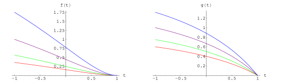
Figure 10: $f(t)=\frac{(t-m_{\pi}^{2})^{2}}{(u-m_{\pi}^{2})^{2}}$ (left panel) and $g(t)=\frac{t-m_{\pi}^{2}}{u-m_{\pi}^{2}}$ (right panel) as the function of $t$ with $S_{1}=3m_{\pi}^{2}$. The bottom (red) curve is for $\theta=\pi/3$, the next (green) curve is for $\theta=\pi/2$ and the second(purple) curve is for $\theta=2\pi/3$ and the top (blue) curve is for $\theta=5\pi/6$. The range of $t$ is $-m_{\pi}^{2}\leq t\leq m_{\pi}^{2}$. The unit of $t$ is $m_{\pi}^{2}$.

Fortunately there is one exception: when the incoming photon is polarized along the direction perpendicular to the scattering plane spanned by $\vec{k}$ and $\vec{r}$, all LO and NLO diagrams with $1/(u-m_{\pi}^{2})$ vanish. Hence the LO, NLO and NNLO pieces of $F_{B}^{1}$ and $F_{B}^{2}$ all vanish in this polarization condition. So, the procedure of extrapolation would be applicable in this particular polarization condition even at the backward angles. Hence one can apply the method of extrapolation to extract $\alpha_{\pi^{\pm}}-\beta_{\pi^{\pm}}$ if the incoming photon is polarized normal to the scattering plane.

VI Discussion and Conclusion

In this section we need address several important issues. The first one is the contribution of nucleon resonances, particularly the contribution of the $\Delta(1232)$. It is well-known that the $\Delta(1232)$ plays an important role in the low-energy phenomenology of the nucleon. It is possible to include its effect systematically in the extended version of HBChPT Delta . Here we only consider the leading order contribution of the $\Delta(1232)$ in ${\cal M}_{H}$. The complete analysis beyond the scope of this article, but the leading order result in ${\cal M}_{H}$ is very instructive. The LO diagrams with the $\Delta(1232)$ are given by: (see Fig. 11)

$${\cal A}_{\Delta}^{a} = \frac{-e^{2}g_{\pi\Delta N}b_{1}}{36M_{N}F_{\pi}}[\tau_{c}-\tau_{3}\delta_{c3}]\frac{1}{\omega_{k}-\Delta}\left\{-(\vec{\epsilon}_{1}\cdot\vec{\epsilon}_{2}^{~{}*})(\vec{\sigma}\cdot\vec{k}~{})+(\vec{\epsilon}_{2}^{~{}*}\cdot\vec{k}~{})(\vec{\sigma}\cdot\vec{\epsilon}_{1})+2i\,\vec{\epsilon}_{2}^{~{}*}\cdot\vec{\epsilon}_{1}\times\vec{k}~{}\right\},$$

$${\cal A}_{\Delta}^{b} = \frac{-e^{2}g_{\pi\Delta N}b_{1}}{36M_{N}F_{\pi}}[\tau_{c}-\tau_{3}\delta_{c3}]\frac{1}{\omega_{q}+\Delta}\left\{-(\vec{\epsilon}_{1}\cdot\vec{\epsilon}_{2}^{~{}*})(\vec{\sigma}\cdot\vec{q}~{})+(\vec{\epsilon}_{1}\cdot\vec{q}~{})(\vec{\sigma}\cdot\vec{\epsilon}_{2}^{~{}*})+2i\vec{\epsilon}_{1}\cdot\vec{\epsilon}_{2}^{~{}*}\times\vec{q}~{}\right\},$$

$${\cal A}_{\Delta}^{c} = \frac{-e^{2}g_{\pi\Delta N}b_{1}}{36M_{N}F_{\pi}}[\tau_{c}-\tau_{3}\delta_{c3}]\frac{1}{\omega_{k}-\omega_{r}-\Delta}\left\{(\vec{\epsilon}_{1}\cdot\vec{\epsilon}_{2}^{~{}*})(\vec{\sigma}\cdot\vec{q}~{})-(\vec{\epsilon}_{1}\cdot\vec{q}~{})(\vec{\sigma}\cdot\vec{\epsilon}_{2}^{~{}*})+2i\,\vec{\epsilon}_{1}\cdot\vec{\epsilon}_{2}^{~{}*}\times\vec{q}~{}\right\},$$

$${\cal A}_{\Delta}^{d} = \frac{-e^{2}g_{\pi\Delta N}b_{1}}{36M_{N}F_{\pi}}[\tau_{c}-\tau_{3}\delta_{c3}]\frac{1}{\omega_{q}+\omega_{r}+\Delta}\left\{(\vec{\epsilon}_{1}\cdot\vec{\epsilon}_{2}^{~{}*})(\vec{\sigma}\cdot\vec{k}~{})-(\vec{\epsilon}_{2}^{~{}*}\cdot\vec{k}~{})(\vec{\sigma}\cdot\vec{\epsilon}_{1})+2i\vec{\epsilon}_{2}^{~{}*}\cdot\vec{\epsilon}_{1}\times\vec{k}~{}\right\},$$

where $\Delta=M_{\Delta}-M_{N}=293MeV$, $g_{\pi\Delta N}$ is the $\pi N\Delta$ coupling constant and $b_{1}$ is the coupling constant of $\gamma N\Delta$ Delta . Large $N_{c}$ QCD gives

$$b_{1}=-\frac{3}{2\sqrt{2}}\kappa_{v},\,\,\,g_{\pi\Delta N}=\frac{3}{2\sqrt{2}}g_{A}.$$ (27)

If $\Delta\gg\omega_{k},\omega_{q},\omega_{r}$, then

$${\cal A}_{\Delta}\simeq\frac{-e^{2}g_{\pi\Delta N}b_{1}}{18M_{N}\Delta F_{\pi}}[\tau_{c}-\delta_{c3}\tau_{3}][(\vec{\epsilon}_{1}\cdot\vec{\epsilon}_{2}^{~{}*})(\vec{\sigma}\cdot\vec{k}-\vec{q}~{})-(\vec{\sigma}\cdot\vec{\epsilon_{1}})(\vec{\epsilon}_{2}^{~{}*}\cdot\vec{k}~{})+(\vec{\sigma}\cdot\vec{\epsilon}_{2}^{~{}*})(\vec{\epsilon}_{1}\cdot\vec{q}~{})].$$ (28)

Comparing with Eq. (16), one finds that it has the same form as Eq. (16). If one assumes that $d_{21}+\frac{d_{22}}{2}$ is saturated by the $\Delta(1232)$ resonance, then one obtains the following estimate:

$$\xi\equiv(4\pi F_{\pi})^{2}\cdot\left(d_{21}+\frac{d_{22}}{2}\right)\simeq-\frac{1}{18}\frac{g_{\pi\Delta N}b_{1}}{M_{N}\Delta}\cdot(4\pi F_{\pi})^{2}\simeq 1.46.$$ (29)

According to the ${\cal O}(p^{4})$ CHPT predictions $\tilde{\alpha}+\tilde{\beta}=0$ and $\tilde{\alpha}-\tilde{\beta}\simeq 1.79$. Including higher order corrections, the ChPT predictions become $\tilde{\alpha}+\tilde{\beta}\simeq 0.12$ and $\tilde{\alpha}-\tilde{\beta}\simeq 1.49$. According to Eq.(18)and Fig. (6-8) the effects due to $\xi$ and the effects due to pion polarizabilities are about the same magnitude. Hence it is necessary to take $\xi$ into consideration when one tries to extract the charged pion polarizabilities from radiative charged pion photoproduction.
There is another important issue to be addressed here. The results of HBChPT for those sub-diagrams such as ${\cal M}_{A}$ and so on are not unique. Because each sub-diagram has at least one off-shell external leg, consequently those amplitudes are changed if the parameterizations of the pion field and the nucleon field are changed. In other words, one can redefine the fields and the results of ${\cal M}_{A}$ to ${\cal M}_{H}$ will be changed. One might worry about the uniqueness of the result. As a matter of fact, there is no ambiguity as long as one uses the same parameterization of the pion and nucleon fields through the whole calculation. Because the physical observables derived from the $S$ matrices with on-shell external legs, are independent of the choice of parameterization of pion and nucleon fields. Note that the explicit forms of the counter terms and the values of the LECs in the chiral Lagrangian are dependent on the choice of the parametrization of the field. Conversely, even if a model is very successful in describing the experimental data of sub-processes such as $\gamma+p\rightarrow\gamma+n+\pi^{+}$, it is not necessarily reliable to use this model to describe the whole process because of the off-shell ambiguity. But there is no such an ambiguity in any effective field theory as long as the physical process is concerned. That is the main advantage of an approach based on an effective field theory.
It is also important to point out that in HBChPT, the convergence of some quantities such as spin polarizabilities, which are extracted from some processes such as spin-dependent Compton scattering off the nucleon, is very poor JKO ; GHM ; KMB . It casts doubt on the convergence of the expansion of the amplitude ${\cal A}$ in Eq.(9). However, it has been shown that the convergence of the differential cross sections for Compton scattering is good MvGovern . The poor convergence of spin polarizabilities is due to the separation of the nucleon pole and non nucleon-pole contribution of the total amplitude. Since here we only concern the total amplitude of radiative charged pion photoproduction, therefore, we should be satisfied without further high-order calculations.
In conclusion, we find that the the main uncertainty in the extraction of pion polarizabilities arises from the effect of two combinations of the low energy constants in the chiral Lagrangian ${\cal L}_{\pi N}^{(3)}$, $d_{20}$ and $d_{21}+\frac{d_{22}}{2}$. Their effects are comparable to the effects of pion polarizabilities on the cross section for radiative charged pion photoproduction. Therefore, a measurement with a large coverage of the scattering angle is required to fit $\xi$, $\eta$ and $\alpha_{\pi^{\pm}}-\beta_{\pi^{\pm}}$ in the backward direction and to fit $\xi$ and $\alpha_{\pi^{\pm}}+\beta_{\pi^{\pm}}$ in the forward direction. We also find the direction of the polarization of the incoming photon plays important role in the extraction. Moreover, the typical extrapolation procedure is severely limited due to diagrams which have pole at $u=m_{\pi}^{2}$ but not at $t=m_{\pi}^{2}$. However such diagrams will vanish when the polarization vector of the incoming photon is perpendicular to the scattering plane. As a result we suggest that the extrapolation is still applicable in this particular situation.

Figure 11: The LO diagrams of radiative pion electroproduction in ${\cal M}_{H}$ in the gauge $\epsilon_{1}\cdot v=\epsilon_{2}\cdot v=0$ with the intermediate $\Delta(1232)$ state.

Appendix A Amplitudes of sub-diagram H

Here we present the amplitudes for the sub-diagrams ${\bf(H)}$. We use the following notation:

$$\frac{1}{i}\int\frac{d^{d}l}{(2\pi)^{d}}\frac{1}{(m_{0}^{2}-l^{2}-i\epsilon)} = \Delta[m_{0}^{2}],$$

$$\frac{1}{i}\int\frac{d^{d}l}{(2\pi)^{d}}\frac{l_{\mu}l_{\nu}}{(m_{0}^{2}-l^{2})^{2}-i\epsilon} = g_{\mu\nu}M_{2}[m_{0}^{2}],$$

$$\frac{1}{i}\int\frac{d^{d}l}{(2\pi)^{d}}\frac{1}{(v\cdot l-A-i\epsilon)(m_{0}^{2}-l^{2}-i\epsilon)} = J_{0}[A,m_{0}^{2}],$$

$$\frac{1}{i}\int\frac{d^{d}l}{(2\pi)^{d}}\frac{l_{\mu}}{(v\cdot l-A-i\epsilon)(m_{0}^{2}-l^{2}-i\epsilon)} = v_{\mu}J_{1}[A,m_{0}^{2}],$$

$$\frac{1}{i}\int\frac{d^{d}l}{(2\pi)^{d}}\frac{l_{\mu}l_{\nu}}{(v\cdot l-A-i\epsilon)(m_{0}^{2}-l^{2}-i\epsilon)} = g_{\mu\nu}J_{2}[A,m_{0}^{2}]+v_{\mu}v_{\nu}J_{3}[A,m_{0}^{2}].$$

Using dimensional regularization one obtains

$$\Delta_{0}[m_{0}^{2}] = 2m_{0}^{2}\left(L+\frac{1}{16\pi^{2}}\ln\frac{m_{0}}{\mu}\right),$$

$$M_{2}[m_{0}^{2}] = \frac{1}{d}\left[\Delta_{0}[m_{0}^{2}]+m_{0}^{2}\cdot\frac{d\Delta_{0}[m_{0}^{2}]}{dm_{0}^{2}}\right],$$

$$J_{0}[A,m_{0}^{2}] = -4AL+\frac{A}{8\pi^{2}}\left(1-2\ln\frac{m_{0}}{\mu}\right)-\frac{1}{4\pi^{2}}\sqrt{m_{0}^{2}-A^{2}}\cdot\cos^{-1}\left(\frac{-A}{m_{0}}\right),$$

$$J_{1}[A,m_{0}^{2}] = A\cdot J_{0}[A,m_{0}^{2}]+\Delta_{0}[m_{0}^{2}],$$

$$J_{2}[A,m_{0}^{2}] = \frac{1}{d-4}\left[(m_{0}^{2}-A^{2})J_{0}[A,m_{0}^{2}]-A\cdot\Delta_{0}[m_{0}^{2}]\right],$$

$$J_{3}[A,m_{0}^{2}] = A\cdot J_{1}[A,m_{0}^{2}]-J_{2}[A,m_{0}^{2}],$$

$$L = \frac{\mu^{d-4}}{16\pi^{2}}\left[\frac{1}{d-4}+\frac{1}{2}\left(\gamma_{E}-1-\ln 4\pi\right)\right],$$

where $\mu$ is the renormalization scale, $\gamma_{E}=0.557215....$ is the Euler number and $d$ is the space-time dimension. Also we define $w=(k-q)^{2}$ and $J^{(m)}_{0}\equiv\frac{\partial^{m}J_{0}[A,m_{0}^{2}]}{\partial(m_{0}^{2})^{m}}$. The results are

$${\cal M}_{H1}=\frac{-\sqrt{2}e^{2}g_{A}^{2}}{2F_{\pi}^{3}}\int^{1}_{0}dy\int^{1-y}_{0}dx$$

$$(\vec{\epsilon_{1}}\cdot\vec{\epsilon}_{2}^{~{}*})(\vec{\sigma}\cdot\vec{k})(x+y)\left[M_{2}^{(1)}[m_{\pi}^{2}+y(y-1)w+xyw]+2\omega_{r}J_{2}^{(2)}[x\omega_{k}+y\omega_{r},m_{\pi}^{2}+y(y-1)w+xyw]\right]$$

$$+ (\vec{\epsilon}_{1}\cdot\vec{\epsilon}_{2}^{~{}*})(\vec{\sigma}\cdot\vec{q})(-y)\left[M_{2}^{(1)}[m_{\pi}^{2}+y(y-1)w+xyw]+2\omega_{r}J_{2}^{(2)}[x\omega_{k}+y\omega_{r},m_{\pi}^{2}+y(y-1)w+xyw]\right]$$

$$+ (\vec{\sigma}\cdot\vec{\epsilon}_{1})(\vec{\epsilon}_{2}^{~{}*}\cdot\vec{k})(x+y-\frac{1}{2})\left[M_{2}^{(1)}[m_{\pi}^{2}+y(y-1)w+xyw]+2\omega_{r}J_{2}^{(2)}[x\omega_{k}+y\omega_{r},m_{\pi}^{2}+y(y-1)w+xyw]\right]$$

$$+ (\vec{\sigma}\cdot\vec{\epsilon}_{2}^{~{}*})(\vec{\epsilon}_{1}\cdot\vec{q})(x+y-1)\left[M_{2}^{(1)}[m_{\pi}^{2}+y(y-1)w+xyw]+2\omega_{r}J_{2}^{(2)}[x\omega_{k}+y\omega_{r},m_{\pi}^{2}+y(y-1)w+xyw]\right]$$

$$+ (\vec{\epsilon_{1}}\cdot\vec{q})(\vec{\epsilon}_{2}^{~{}*}\cdot\vec{k})(\vec{\sigma}\cdot\vec{k})[y(x+y)(x+y-1)]\left[\Delta_{0}^{(2)}[m_{\pi}^{2}+y(y-1)w+xyw]+2\omega_{r}J_{0}^{(2)}[x\omega_{k}+y\omega_{r},m_{\pi}^{2}+y(y-1)w+xyw]\right]$$

$$- (\vec{\epsilon}_{1}\cdot\vec{q})(\vec{\epsilon}_{2}^{~{}*}\cdot\vec{k})(\vec{\sigma}\cdot\vec{q})y^{2}(x+y-1)\left[\Delta_{0}^{(2)}[m_{\pi}^{2}+y(y-1)w+xyw]+2\omega_{r}J_{0}^{(2)}[x\omega_{k}+y\omega_{r},m_{\pi}^{2}+y(y-1)w+xyw]\right]$$

$${\cal M}_{H2}=\frac{-\sqrt{2}e^{2}g_{A}^{2}}{2F_{\pi}^{3}}\int^{1}_{0}dy\int^{1-y}_{0}dx$$

$$(\vec{\epsilon}_{1}\cdot\vec{\epsilon}_{2}^{~{}*})(\vec{\sigma}\cdot\vec{q})(x+y)\left[M_{2}^{(1)}[m_{\pi}^{2}+y(y-1)w+xyw]-2\omega_{r}J_{2}^{(2)}[x\omega_{q}-y\omega_{r},m_{\pi}^{2}+y(y-1)w+xyw]\right]$$

$$+ (\vec{\epsilon}_{1}\cdot\vec{\epsilon}_{2}^{~{}*})(\vec{\sigma}\cdot\vec{k})(-y)\left[M_{2}^{(1)}[m_{\pi}^{2}+y(y-1)w+xyw]-2\omega_{r}J_{2}^{(2)}[x\omega_{q}-y\omega_{r},m_{\pi}^{2}+y(y-1)w+xyw]\right]$$

$$+ (\vec{\sigma}\cdot\vec{\epsilon}_{2}^{~{}*})(\vec{\epsilon}_{1}\cdot\vec{q})(x+y-\frac{1}{2})\left[M_{2}^{(1)}[m_{\pi}^{2}+y(y-1)w+xyw]-2\omega_{r}J_{2}^{(2)}[x\omega_{q}-y\omega_{r},m_{\pi}^{2}+y(y-1)w+xyw]\right]$$

$$+ (\vec{\sigma}\cdot\vec{\epsilon}_{1})(\vec{\epsilon}_{2}^{~{}*}\cdot\vec{k})(x+y-1)\left[M_{2}^{(1)}[m_{\pi}^{2}+y(y-1)w+xyw]-2\omega_{r}J_{2}^{(2)}[x\omega_{q}-y\omega_{r},m_{\pi}^{2}+y(y-1)w+xyw]\right]$$

$$+ (\vec{\epsilon}_{2}^{~{}*}\cdot\vec{k})(\vec{\epsilon}_{1}\cdot\vec{q})(\vec{\sigma}\cdot\vec{q})[y(x+y)(x+y-1)]\left[\Delta_{0}^{(2)}[m_{\pi}^{2}+y(y-1)w+xyw]-2\omega_{r}J_{0}^{(2)}[x\omega_{q}-y\omega_{r},m_{\pi}^{2}+y(y-1)w+xyw]\right]$$

$$- (\vec{\epsilon}_{2}^{~{}*}\cdot\vec{k})(\vec{\epsilon}_{1}\cdot\vec{q})(\vec{\sigma}\cdot\vec{k})y^{2}(x+y-1)\left[\Delta_{0}^{(2)}[m_{\pi}^{2}+y(y-1)w+xyw]-2\omega_{r}J_{0}^{(2)}[x\omega_{q}-y\omega_{r},m_{\pi}^{2}+y(y-1)w+xyw]\right]$$

$${\cal M}_{H3} = \frac{\sqrt{2}e^{2}g_{A}^{2}}{4F_{\pi}^{3}}(\vec{\sigma}\cdot\vec{k}-\vec{q})(\vec{\epsilon}_{1}\cdot\vec{\epsilon}_{2}^{~{}*})\int^{1}_{0}dxx\cdot\{\Delta_{0}^{(1)}[m_{\pi}^{2}+x(x-1)w]+2\omega_{r}J_{0}^{(1)}[x\omega_{r},m_{\pi}^{2}+x(x-1)w]\}.$$

$${\cal M}_{H4} = -\frac{\sqrt{2}e^{2}g_{A}^{2}}{4F_{\pi}^{3}}(\vec{\sigma}\cdot\vec{k}-\vec{q})(\vec{\epsilon}_{1}\cdot\vec{\epsilon}_{2}^{~{}*})\int^{1}_{0}dx(1-x)\cdot\{\Delta_{0}^{(1)}[m_{\pi}^{2}+x(x-1)w]+2\omega_{r}J_{0}^{(1)}[(x-1)\omega_{r},m_{\pi}^{2}+x(x-1)w]\}.$$

$${\cal M}_{H5}={\cal M}_{H6}=0.$$ (36)

$${\cal M}_{H7} = -\frac{\sqrt{2}e^{2}g_{A}^{2}}{F_{\pi}^{3}}(\vec{\sigma}\cdot 3\vec{k}-3\vec{q}-2\vec{r})\{(\vec{\epsilon}_{1}\cdot\vec{\epsilon}_{2}^{~{}*})\int^{1}_{0}dy\int^{1-x}_{0}dy(-1)\cdot M_{2}^{(1)}[m_{\pi}^{2}+y(y-1)w+xyw]$$ (37)

$$+ (\vec{\epsilon}_{1}\cdot\vec{q})(\vec{\epsilon}_{2}^{~{}*}\cdot\vec{k})\int^{1}_{0}dy\int^{1-x}_{0}dy~{}y(1-x-y)\Delta_{0}^{(2)}[m_{\pi}^{2}+y(y-1)w+xyw]\}.$$

$${\cal M}_{H8} = \frac{\sqrt{2}e^{2}g_{A}^{2}}{2F_{\pi}^{3}}(\vec{\sigma}\cdot 3\vec{k}-3\vec{q}-2\vec{r})(\vec{\epsilon}_{1}\cdot\vec{\epsilon}_{2}^{~{}*})\int^{1}_{0}dx(-1)\cdot\{\Delta^{(1)}_{0}[m_{\pi}^{2}+x(x-1)w]\}.$$ (38)

$${\cal M}_{H9}=\frac{\sqrt{2}e^{2}}{F_{\pi}}(d_{21}+\frac{d_{22}}{2})[(\vec{\epsilon_{1}}\cdot\vec{\epsilon}_{2}^{~{}*})(\vec{\sigma}\cdot\vec{k}-\vec{q}~{})-(\vec{\sigma}\cdot\vec{\epsilon}_{1})(\vec{\epsilon}_{2}^{*}\cdot\vec{k}~{})+(\vec{\sigma}\cdot\vec{\epsilon}_{2}^{~{}*})(\vec{\epsilon_{1}}\cdot\vec{q})]$$ (39)

Here we do not explicitly display the results of cross diagrams which can be obtained by exchanging $\vec{k}\longleftrightarrow-\vec{q},\,\,\vec{\epsilon}_{1}\longleftrightarrow\vec{\epsilon}_{2}^{~{}*}.$

References

• (1) J. Bijenens and F. Cornet, Nucl. Phys. B 296, 557 (1988); J. F. Donoghue, B. R. Holstein, Phys. Rev. D 40, 2378 (1989); B. R. Holstein, Comm. Nucl. Part. Phys. A 19, 221 (1990).
• (2) J. Gasser and H. Leutwyler, Annals Phys. 158, 142 (1984).
• (3) E. Frle$\breve{z}$ et al., Phys. Rev. Lett, 93 181804 (2004).
• (4) S. Bellucci, J. Gasser and M. E. Sainio, Nucl. Phys. B 423 80 (1994).
• (5) U. Bürgi, Nucl. Phys. 479, 392 (1996).
• (6) W. Detmold, B. C. Tiburzi and A. Walker-Loud, talk given at 26th International Symposium on Lattice Field Theory (Lattice 2008), Williamsburg, Virginia, 14-20 Jul 2008, e-print. arXiv:0809.0721.
• (7) Yu. M. Antipov et al., Phys. Lett. B 121, 445 (1983); Z. Phys. C 26, 495 (1985).
• (8) T. Aibergenov et al., Proc. of the Lebedev Phys. Inst. 186, 169 (1988).
• (9) J. Boyer et al., Phys. Rev. D 42, 1350 (1990).
• (10) D. Babusci, S. Bellucci, G. Giordano, G. Matone, A. M. Sandorfi, M. A. Moinester, Phys. Lett. B 277, 158 (1992).
• (11) J. Ahrens et al., Eur. Phys. J. A 23, 113 (2005).
• (12) J. Gasser, M. A. Ivanov and M. E. Sainio, Nucl. Phys. B 745, 84 (2006).
• (13) V. Bernard, N. Kaiser and Ulf-G. Meissner, Int. J. Mod. Phys E 4, 193 (1995).
• (14) L. Fil’kov , Sov. J. Nucl. Phys. 41, 636 (1985).
• (15) D. Drechsel and L. Fil’kov, Z. Phys. A 349, 177 (1994).
• (16) G. Chew et al., Phys. Rev. 106, 1345 (1957).
• (17) C.-W. Kao, in preparation.
• (18) N. Fettes, Ulf-G. Meissner, Nucl. Phys. A676, 311 (2000).
• (19) C. Unkmeir, A. Ocherachvili, T. Fuchs, M. A. Moinester, S. Scherer, Phys. Rev. C 65, 015206 (2001).
• (20) C. Unkmeir, S. Scherer, A. I. L’vov and D. Drechsel, Phys. Rev. D 61, 034002 (1999).
• (21) H. W. Fearing, T. R. Hemmert, R. Lewis and C. Unkmeir, Nucl. Phys. A 684, 377 (2001); Phys. Rev. C62, 054006 (2000).
• (22) V. Bernard, N. Kaiser, J. Kambor and Ulf-G. Meissner, Nucl. Phys. B 388, 315( 1992).
• (23) J. Wess and B. Zumino, Phys. Lett. B37, 95 (1971); E. Witten, Nucl. Phys. B 223, 422 (1983).
• (24) J. S. Bell and R. Jackiw, Nuovo Cimento 60A, 47 (1969); S. Adler, Phys. Rev. 177, 2426 (1969).
• (25) Y. Kim, F. Myhrer and K. Kubodera, Prog. Theor. Phys.  112, 289 (2004).
• (26) N. Fettes,U. Meissner, and S. Steininger, Ann. Phys. 283, 273(2000), Erratum-ibid. 288, 249 (2001).
• (27) T. R. Hemmert, B. R. Holstein and J. Kambor, J. Phys. G24, 1831 (1998).
• (28) X. Ji, C.-W Kao and J. Osborne, Phys. Rev D 61, 074003 (2000).
• (29) G. C. Gellas, T. R. Hemmert and U. -G. Meissner, Phys. Rev. Lett. 85, 14(2000).
• (30) K. B. V. Kummar, J. A. McGovern and M. C. Birse, Phys. Lett. B 479, 167(2000).
• (31) J.  A. McGovern, Phys.Rev.C 63 064608 (2001), Erratum-ibid.C 66, 039902 (2002).
• (32) C.-W. Kao, Int. Mod. Phys. A 21, 2027(2006).