Composite Vector Mesons and the Little Higgs Mechanism

Abstract

I review a technique to embed vector mesons in the chiral Lagrangian of QCD, and apply it to more general coset spaces, relevant for Little Higgs models. The implementation of heavy spin-1 fields in Little Higgs models allows for a better control over previously non calculable, ultra-violate sensitive quantities, such as the Higgs couplings. A relevant application is the study of vacuum alignment in the $SU(6)/Sp(6)$ models.

Physics Department, Sloane Laboratory, Yale University
New Haven CT 06520, U.S.
E-mail: maurizio.piai@yale.edu

In Little Higgs (LH) models, the Higgs fields are pseudo-Nambu-Goldstone bosons (PNGS) of an approximate global symmetry. This is an effective field theory, providing a description valid up to the cut-off scale $\Lambda\sim 4\pi f$, where $f$ is the symmetry-breaking scale. The symmetry structure of the models is such that the Higgs mass can be radiatively generated only by loop diagrams involving more than one of the symmetry-breaking couplings, thus suppressing it in respect to its natural size.

Some relevant quantities are quadratically sensitive to the cut-off of the theory. In [?], it has been shown that calculability can be improved by including in the spectrum of the effective theory heavy spin-1 fields, to be thought of as heavy resonances of the underlying (strong dynamics) UV completion. The mechanism proposed is based on the idea of hidden symmetry [?], and its use in the QCD chiral Lagrangian. A crucial role is played by the vector limit [?], as a point of enhanced symmetry of the models, and by locality in the theory-space language [?,?].

1 Vector Mesons and the QCD Chiral Lagrangian.

At low energies, 2-flavor QCD is well described by an effective Lagrangian containing the PNGB’s of the broken phase (identified with the physical pions), describing the fluctuations along the broken generators in the coset $SU(2)_{L}\times SU(2)_{R}/SU(2)_{V}$. An effective Lagrangian contains in general also explicit symmetry breaking terms, such as gauge interactions ($U(1)_{\rm em}\subset SU(2)_{V}$), mass terms (quark masses), and possible Wess-Zumino terms [?]. I focus here on gauge interactions, neglecting other symmetry breaking terms. The symmetry structure of the Lagrangian can be represented by a 2-site and 1-link diagram in the theory-space language, in which the $D=4$ Lagrangian describes a $D=5$ theory, with a discrete fifth dimension. Locality means allowing only nearest-neighbor interactions in the fifth dimension.

To introduce in the spectrum the $\rho$ mesons of QCD, one rewrites the theory as a 3-site 2-link model, with an additional gauged $SU(2)$, so that the coset-space structure becomes $SU(2)_{L}\times SU(2)_{\rho}\times SU(2)_{R}/SU(2)_{V}$. The Lagrangian contains

$${\cal L}\,=\,\frac{f^{2}}{4}\,\left(\mbox{Tr}\,|D^{\mu}\Sigma_{L}|^{2}+\mbox{Tr}\,|D^{\mu}\Sigma_{R}|^{2}+\,\frac{\kappa}{2}\,\mbox{Tr}\,|D^{\mu}(\Sigma_{L}\Sigma_{R})|^{2}\right)\,+\cdots,$$ (1)

plus the Yang-Mills terms for the $U(1)$ and $SU(2)_{\rho}$ gauge fields. The gauge bosons acquire mass via spontaneous symmetry breaking: half of the $\pi_{i}$ fields contained in $\Sigma_{L,R}\equiv\exp(i\pi_{L,R}/f)$ become, in unitary gauge, the longitudinal components of the massive $\rho$ fields. The spectrum of the model contains then the physical pions, with a decay constant $f_{\pi}=\sqrt{\frac{1+\kappa}{2}}f$, the massless photon with coupling $e$, and three $\rho$ mesons with masses proportional to the gauge coupling $g_{\rho}$. The electromagnetic $U(1)_{\rm em}$ is generated by a linear combination of the generators of the gauged $U(1)\subset SU(2)_{L}\times SU(2)_{R}$ and $SU(2)_{\rho}$, with mixing angle $\cos^{2}\theta\approx\Big{(}1-\frac{e^{2}}{g_{\rho}^{2}}\Big{)}$.

One can use this Lagrangian to compute the Coleman-Weinberg (CW) 1-loop potential [?], from which one can read the splitting between neutral- and charged-pion masses in terms of the cut-off scale $\Lambda$ and of the mass of $\rho$’s [?]:

$$\delta m^{2}_{\pi^{\pm}}\simeq\frac{3e^{2}}{16\pi^{2}(1+\kappa)}\Big{(}\frac{\kappa\Lambda^{2}}{\cos^{2}\theta}+m^{2}_{\rho^{0}}\log\frac{\Lambda^{2}}{m^{2}_{\rho^{0}}}+\cdots\Big{)}.$$ (2)

The procedure can be generalized, including more sites and hence more spin-1 resonances.

Consider the limit $\kappa\rightarrow 0$. The Lagrangian becomes local in the theory space language. As a consequence (see Eq. (2)), the quadratic divergence disappears, in favor of a milder logarithmic divergence. In the local limit, the CW potential is less UV-sensitive, and observable quantities can be better understood in terms of low-energy degrees of freedom. Further, $\kappa\rightarrow 0$ represents a point of enhanced symmetry: the chiral symmetry is restored to a global $SU(2)^{2}$ connecting the physical pions and the longitudinal components of the $\rho$’s. This is the vector limit introduced first in [?]. Ordinary QCD is probably not too close to the vector limit (one can estimate $\kappa\sim 1/3$). In a general effective theory, locality and vector limit are not controlled by the same parameter, and have to be considered as distinct properties.

2 Vacuum Alignment in $SU(6)/Sp(6)$

In LH models based on the general coset $G/H$, heavy spin-1 states can be implemented in analogy to the QCD case. This allows to discuss physically relevant quantities, such as the mass and couplings of the Higgs fields, the scale of unitarity violation [?] and vacuum alignment. I focus here on the last issue, in the interesting example of $SU(6)/Sp(6)$ [?].

The $SU(6)$ global symmetry is broken by an antisymmetric condensate to its $Sp(6)$ subgroup. Two $SU(2)_{1,2}$ groups are gauged (I neglect the abelian $U(1)$’s here), and the spontaneous breaking leaves only the diagonal $SU(2)_{L}$ unbroken. Of the PNGB’s, three are eaten in the generation of the mass of the $W^{\prime}$ gauge bosons, the others arrange in two Higgs doublets, one complex singlet $\eta$ and possible axion fields. Several variations of the original model have been discussed, in connection with precision electroweak physics [?], or in order to describe flavor physics [?].

A simple analysis suggests that this choice of the vacuum is unstable: vacuum alignment seems to favor the unbroken $Sp(6)$ to contain the two $SU(2)$’s [?]. This can be seen from the fact that the complex singlet field acquires a negative, quadratically divergent mass term in the 1-loop CW potential. But the quadratic divergence implies that this is a UV-dominated, not calculable quantity.

Consider instead the case in which one introduces in the spectrum the first three spin-1 modes, namely two copies $\rho$ and $\rho^{\prime}$ of techni-rho’s and one copy of techni-$a_{1}$’s, with $m_{\rho}<m_{a_{1}}<m_{\rho^{\prime}}$. The construction is described in Fig. 1.

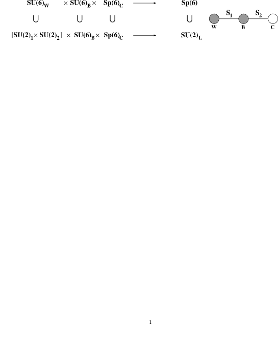
Figure 1: Symmetry structure and diagrammatic representation of the $SU(6)/Sp(6)$ model with inclusion of $\rho$, $a_{1}$ and $\rho^{\prime}$ states. See text for details.

The global symmetry is enlarged to a 3-site 2-link model, in which $SU(6)_{B}\times Sp(6)_{C}$ is gauged, together with the $SU(2)^{2}$ subgroup of $SU(6)_{W}$. The breaking to $Sp(6)$ leaves only an $SU(2)_{L}$ combination unbroken. The lowest-order terms in the Lagrangian (Yang-Mills kinetic terms are understood) are

$${\cal L} = f^{2}\Big{(}\mbox{Tr}\,|DS_{1}|^{2}+c^{2}\mbox{Tr}\,|DS_{2}|^{2}$$ (3)

$$+ \kappa_{1}\mbox{Tr}\,|DS_{1}S_{2}|^{2}+\frac{\kappa_{2}}{4}\mbox{Tr}\,|DS_{2}\Sigma_{0}S_{2}^{T}|^{2}+\frac{\kappa^{\prime}}{4}\mbox{Tr}\,|DS_{1}S_{2}\Sigma_{0}S_{2}^{T}S_{1}^{T}|^{2}\Big{)}\,,$$

where $S_{j}=e^{i\,\pi_{j}/f}$. The dimensionless constants $c^{2}$, $\kappa_{1}$, $\kappa_{2}$, $\kappa^{\prime}$, as well as the gauge couplings $g_{1}$, $g_{2}$, $g_{B}$, $g_{C}$ in the covariant derivatives, are determined by the (unknown) underlying dynamics. In unitary gauge, all the components of $\pi_{i}$ in $Sp(6)$ disappear to form longitudinal components of the $\rho$ and $\rho^{\prime}$ fields. One linear combination of the PNGB’s in the coset $SU(6)/Sp(6)$ is eaten to give mass to the $a_{1}$ fields. Of the other linear combination, three components give mass to the heavy $W^{\prime}$ bosons, while the others are the light pseudo-scalar states to be identified with the scalar sector of the theory.

For simplicity, one can set $c^{2}=1$. The couplings $\kappa_{1}$ and $\kappa^{\prime}$ are non-local in the theory space description. Setting them to zero gives a finite 1-loop CW potential for the $\eta$ field, which reads:

$$V(\eta)\,=\,V_{1}\,f^{4}\,\cos\left(\frac{|\eta|}{F_{\eta}}\right)\,,$$ (4)

where the decay constant $F_{\eta}$ depends on $\kappa_{2}$ and $f$, and where constant terms and higher order terms in the Fourier expansion have been neglected. $V_{1}$ can be computed exactly. The vector limit requires also $\kappa_{2}=0$. How far from the vector limit must the theory be, in order for the (finite) coefficient of the mass term for $\eta$ to turn positive, and the vacuum to be stable? The answer is depicted in Fig. 2.

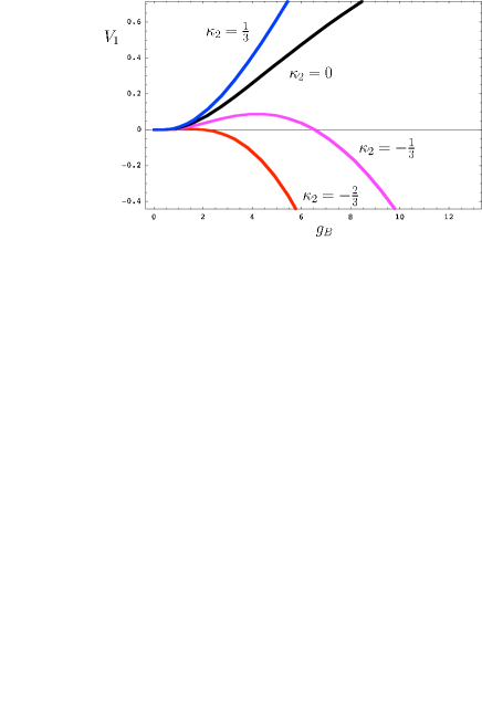
Figure 2: The coefficient $V_{1}$ in the CW 1-loop potential for the field $\eta$ in Eq. (4) as a function of $g_{B}$ for different values of $\kappa_{2}$. All curves are computed for $\kappa^{\prime}=\kappa_{1}=0$, $c^{2}=1$, $g_{1}=0.65$, $g_{2}=3.3$, $g_{C}=5.2$.

The $\rho$ and $\rho^{\prime}$ contributions to $V_{1}$ are positive, while $a_{1}$ contributes negatively. For appropriate choices of the parameters, mixing effects become important, and the $\rho$’s contribute less than the heavier $a_{1}$’s, so that the vacuum may be stable. To be more specific, for vanishing or positive values of $\kappa_{2}$, $V_{1}$ is a positive definite quantity and the vacuum unstable. For negative values of $\kappa_{2}$, and for large values of $g_{B}$ (a region of parameter space where the theory is close to the strong coupling regime, and hence perturbative results have to be interpreted cautiously), $V_{1}$ turns negative, thus showing on a computable example that the naif expectation of vacuum alignment can, in principle, be modified without invoking the underlying dynamics.

3 Acknowledgements

I thank the organizers for partial support, and A. Pierce and J. Wacker for the collaboration this work is based upon. Research supported by the grant DE-FG02-92ER-4074.

References

- [1] M. Piai, A. Pierce and J. Wacker, hep-ph/0405242.
- [2] M. Bando et al., Phys. Rev. Lett. 54, 1215 (1985); M. Bando et al., Phys. Rept. 164, 217 (1988); M. Harada and K. Yamawaki, Phys. Rept. 381, 1 (2003).
- [3] H. Georgi, Nucl. Phys. B 331, 311 (1990).
- [4] N. Arkani-Hamed et al., Phys. Rev. Lett. 86, 4757 (2001); C. T. Hill et al., Phys. Rev. D 64, 105005 (2001).
- [5] D. T. Son and M. A. Stephanov, Phys. Rev. D 69, 065020 (2004);
- [6] J. Wess and B. Zumino, Phys. Lett. B 37, 95 (1971); E. Witten, Nucl. Phys. B 223, 422 (1983). See also M. Fabbrichesi et al., Phys. Rev. D 66, 105028 (2002).
- [7] S. R. Coleman and E. Weinberg, Phys. Rev. D 7, 1888 (1973).
- [8] M. Harada et al. Phys. Lett. B 568, 103 (2003).
- [9] See also M. Harada, F. Sannino and J. Schechter, Phys. Rev. D 69, 034005 (2004).
- [10] I. Low, W. Skiba and D. Smith, Phys. Rev. D 66, 072001 (2002);
- [11] E. g. T. Gregoire, D. R. Smith and J. G. Wacker, Phys. Rev. D 69, 115008 (2004).
- [12] F. Bazzocchi et al., Phys. Rev. D 68, 096007 (2003); ibid. 69, 036002 (2004).
- [13] M. E. Peskin, Nucl. Phys. B 175, 197 (1980); J. Preskill, ibid. 177, 21 (1981).