Symmetry Nonrestoration at High Temperature in Little Higgs Models

A detailed study of the high temperature dynamics of the scalar sector of Little Higgs scenarios, proposed to stabilize the electroweak scale, shows that the electroweak gauge symmetry remains broken even at temperatures much larger than the electroweak scale. Although we give explicit results for a particular modification of the Littlest Higgs model, we expect that the main features are generic. As a spin-off, we introduce a novel way of dealing with scalar fluctuations in nonlinear sigma models, which might be of interest for phenomenological applications.

September 2004

IFT-UAM/CSIC-04-44

CI-UAN/04-07FT

hep-ph/0409070

1 Introduction

Little Higgs (LH) models [1, 2, 3, 4] provide a new scenario for electroweak symmetry breaking which stabilizes the electroweak scale. It is well known that symmetries in the Standard Model (SM) Lagrangian force gauge bosons and fermions to be massless. The main feature of LH models is the inclusion of additional global symmetries which force the Higgs boson mass to be zero. The incorporation of explicit violations of these symmetries in a precise way explains why the ratio of the Higgs mass to the cutoff of the theory, $m_{H}^{2}/\Lambda^{2}$, is small: the Little Higgs boson is a naturally light pseudo-Goldstone boson [2].

Below the cutoff scale $\Lambda\sim 10$ TeV, there are additional particles (with masses of order $f\sim 1$ TeV) which cancel the quadratically divergent contributions to the Higgs boson mass from SM particles (or at least the most dangerous ones). Beneath the TeV scale the effective degrees of freedom are those of the Standard Model. The initial implementation of this idea was based on a SU(5)/SO(5) nonlinear sigma model which contained a gauged $[SU(2)\times U(1)]^{2}$ subgroup. However, this model is in conflict with low-energy precision electroweak measurements and from direct searches for a $Z^{\prime}$ boson [5, 6, 7, 8, 9], both problems being related to the additional $U(1)$ gauge group. Although this problem is not of direct concern for our purposes, we focus in this paper on a Little Higgs model which is a simple variation of the so-called Littlest one, having only a gauged $SU(2)\times SU(2)\times U(1)$ group [10]. The performance of the model with respect to electroweak fits is improved while the smallness of the $g^{\prime}$ coupling tames the remnant quadratic divergence in the Higgs boson mass associated to the $U(1)_{Y}$ gauge group.

In this paper we study the finite temperature behaviour of Little Higgs models. The main motivation is related to the peculiar way in which such models cancel the quadratically divergent corrections to the Higgs boson mass. As is well known, in the early Universe the Higgs scalar field gets an effective thermal mass (squared) $m_{eff}^{2}\sim T^{2}$ from interactions with the ambient hot plasma. It is this positive $m_{eff}^{2}$ which is responsible for symmetry restoration at high temperature [12]. This effective mass can be computed diagrammatically using well established finite temperature techniques; the self-energy diagrams which are quadratically divergent at $T=0$ are precisely the ones that give a contribution to the Higgs thermal mass. The correspondence is very simple [13]: a one-loop bosonic self-energy diagram that gives $\delta m_{h}^{2}=\kappa\Lambda^{2}/(16\pi^{2})$, where $\Lambda$ is an UV cutoff, produces $\delta m_{eff}^{2}=\kappa T^{2}/12$ at finite temperature. For a fermionic one-loop self-energy diagram, if the zero $T$ result is $\delta m_{h}^{2}=-\kappa\Lambda^{2}/(16\pi^{2})$, the finite $T$ contribution of the same diagram will be $\delta m_{eff}^{2}=\kappa T^{2}/24$. For instance, in the Standard Model one gets the well known quadratically divergent correction to the Higgs mass

$$\delta m_{h}^{2}={3\Lambda^{2}\over 16\pi^{2}}\left[2\lambda+{1\over 2}g^{2}+{1\over 4}(g^{2}+{g^{\prime}}^{2})-2h_{t}^{2}\right]\ ,$$ (1)

where $\lambda$ is the Higgs quartic coupling (normalized so as to have $m_{h}^{2}=2\lambda v^{2}$ with $v=246$ GeV), $g$ is the $SU(2)$ gauge coupling, $g^{\prime}$ the $U(1)_{Y}$ coupling and $h_{t}$ the top Yukawa coupling. The result (1) translates, at $T\neq 0$, into

$$\delta m_{eff}^{2}={T^{2}\over 4}\left[2\lambda+{1\over 2}g^{2}+{1\over 4}(g^{2}+{g^{\prime}}^{2})+h_{t}^{2}\right]\ .$$ (2)

In the MSSM, although the sum of quadratically divergent corrections to $m_{h}^{2}$ cancels between bosonic and fermionic degrees of freedom, the corresponding corrections at $T\neq 0$ do not and one gets symmetry restoration also in that case.

The defining property of Little Higgs models is that quadratically divergent corrections to $m_{h}^{2}$ cancel sector by sector in the model, between particles of the same statistics. At $T\neq 0$ this leads one to expect that $\delta m_{eff}^{2}$ will also be zero in this type of models. Notice though that this will only happen for sufficiently large temperatures, such that the heavy partners of the SM particles are thermally produced and populate the hot plasma. At low temperatures we expect the heavy particles with mass $\sim f$ to be Boltzmann decoupled, and we find the same SM $T^{2}$ dependence on the Higgs mass, with the electroweak symmetry being restored as usual. (That is, the electroweak phase transition will take place as in the SM, at $T\sim 100$ GeV.) As the temperature approaches $f\sim 1$ TeV the new particles introduced in Little Higgs models will be in thermal equilibrium in the plasma, the thermal Higgs mass will drop to zero and the electroweak symmetry will be broken again. Although these expectations will prove to be correct, they concern the behaviour of the Higgs potential, $V(h)$, for small values of the Higgs field $h$. In order to study what happens to the minimum of the Higgs potential at $T\simeq f\sim 1$ TeV, we will need to study larger values of $h$.

Without knowing the UV theory that supersedes the Little Higgs model beyond $\Lambda\simeq 4\pi f$ we cannot study the behaviour of our theory at $T\geq\Lambda/\pi\sim 4f$ (at such temperatures the free-energy contribution from particles with mass $\sim\Lambda$ is no longer negligible). With this limitation in mind, we would like to explore in this paper the behaviour of the Higgs potential of Little Higgs models at finite temperature. We will confirm the expected behaviour described in the previous paragraph and discover some peculiar features in the temperature evolution of $V(h)$. We present detailed results for the model of ref. [10] but expect that the main features we find are generic as they are based on the defining properties of Little Higgs models.

In section 2 we present the model and our notation. Section 3 describes in detail the structure of the zero temperature effective potential at one-loop order, paying particular attention to the treatment of the contributions from scalar fluctuations. Section 4 then goes on to compute the finite temperature effective potential and describes some interesting features of its temperature evolution. In particular, we discover that the electroweak gauge symmetry remains broken even if the system is heated up to temperatures larger than the electroweak scale. In section 5 we present some conclusions. Appendix A contains explicit expressions for the mass matrices of the different species of particles in the model, calculated to all orders in the Higgs background, which are necessary to compute the one-loop effective potential. Appendix B deals with the behaviour of the potential along the direction of the triplet field contained in the model.

2 The Little Higgs Model

The model is based on the $SU(5)/SO(5)$ nonlinear sigma model of [2] (the Littlest Higgs), modified according to [10]. The spontaneous breaking of $SU(5)$ down to $SO(5)$ is produced by the vacuum expectation value (vev) of a $5\times 5$ symmetric matrix $\Phi$ [which transforms under $SU(5)$ as $\Phi\rightarrow U\Phi U^{T}$] for instance when $\langle\Phi\rangle=I_{5}$ (we denote by $I_{n}$ the $n\times n$ identity matrix). This breaking of the global $SU(5)$ symmetry produces 14 Goldstone bosons among which lives the scalar Higgs field. Instead of working on the background $\langle\Phi\rangle=I_{5}$ we follow [2] and, making a basis change, we choose $\langle\Phi\rangle=\Sigma_{0}$ where

$$\Sigma_{0}=\left(\begin{array}[]{ccc}0&0&I_{2}\\ 0&1&0\\ I_{2}&0&0\end{array}\right)\ .$$ (3)

Calling $U_{0}$ the $SU(5)$ matrix that performs this change of basis, we have $\Sigma_{0}=U_{0}U_{0}^{T}$ while all the group generators change as $t_{a}=U_{0}t_{a}^{(0)}U_{0}^{\dagger}$ [$t_{a}^{(0)}$ are the generators in the original basis]. The unbroken $SO(5)$ generators satisfied the obvious relation $T_{a}^{(0)}+T_{a}^{(0)T}=0$ and multiplying on the left by $U_{0}$ and on the right by $U_{0}^{T}$ we arrive at the condition

$$T_{a}\Sigma_{0}+\Sigma_{0}T_{a}^{T}=0\ ,$$ (4)

for the generators in the new basis (a condition which is immediate to obtain alternatively just by requiring invariance of $\Sigma_{0}$). In the original basis the broken generators obviously satisfy $X_{a}^{(0)}=X_{a}^{(0)T}$. Multiplying again by $U_{0}$ and $U_{0}^{T}$ one gets in the transformed basis

$$X_{a}\Sigma_{0}=\Sigma_{0}X_{a}^{T}\ .$$ (5)

The Goldstone bosons can be parametrized through the nonlinear sigma model field

$$\Sigma=e^{i\Pi/f}\Sigma_{0}e^{i\Pi^{T}/f}=e^{2i\Pi/f}\Sigma_{0},$$ (6)

where $\Pi=\sum_{a}\Pi^{a}X^{a}$. The model assumes a gauged $SU(2)_{1}\times SU(2)_{2}\times U(1)_{Y}$ subgroup of $SU(5)$ with generators

$$Q_{1}^{a}=\left(\begin{array}[]{cc}\sigma^{a}/2&0_{2\times 3}\\ 0_{3\times 2}&0_{3\times 3}\end{array}\right)\ ,\hskip 14.22636ptQ_{2}^{a}=\left(\begin{array}[]{cc}0_{3\times 3}&0_{3\times 2}\\ 0_{2\times 3}&-\sigma^{a^{*}}/2\end{array}\right)\ ,$$ (7)

(where $\sigma^{a}$ are the Pauli matrices) and $Y={\mathrm{d}iag}(1,1,0,-1,-1)/2$. The vacuum expectation value in eq. (3) additionally breaks $SU(2)_{1}\times SU(2)_{2}$ down to the SM $SU(2)$ group.

The hermitian matrix $\Pi$ in eq. (6) contains the Goldstone and (pseudo)-Goldstone bosons:

$$\Pi=\left(\begin{array}[]{ccc}\xi&\frac{H^{\dagger}}{\sqrt{2}}&\phi^{\dagger}\\ \frac{H}{\sqrt{2}}&0&\frac{H^{*}}{\sqrt{2}}\\ \phi&\frac{H^{T}}{\sqrt{2}}&\xi^{T}\end{array}\right)+{1\over\sqrt{20}}\zeta^{0}{\mathrm{d}iag}(1,1,-4,1,1)\ ,$$ (8)

where $H=(h^{0},h^{+})$ is the Higgs doublet; $\phi$ is a complex $SU(2)$ triplet given by the symmetric $2\times 2$ matrix:

$$\phi=\left[\begin{array}[]{cc}\phi^{0}&{1\over\sqrt{2}}\phi^{+}\\ {1\over\sqrt{2}}\phi^{+}&\phi^{++}\end{array}\right]\ ,$$ (9)

the field $\zeta^{0}$ is a singlet and finally, $\xi$ is the real triplet of Goldstone bosons associated to $SU(2)_{1}\times SU(2)_{2}\rightarrow SU(2)$ breaking:

$$\xi={1\over 2}\sigma^{a}\xi^{a}=\left[\begin{array}[]{cc}{1\over 2}\xi^{0}&{1\over\sqrt{2}}\xi^{+}\\ {1\over\sqrt{2}}\xi^{-}&-{1\over 2}\xi^{0}\end{array}\right]\ .$$ (10)

The kinetic part of the Lagrangian is

$${\cal L}_{k}=\frac{f^{2}}{8}{\mathrm{T}r}[(D_{\mu}\Sigma)(D^{\mu}\Sigma)^{\dagger}]$$ (11)

where

$$D_{\mu}\Sigma=\partial_{\mu}\Sigma-i\sum_{j=1}^{2}g_{j}W_{j}^{a}(Q_{j}^{a}\Sigma+\Sigma Q_{j}^{aT})-ig^{\prime}B_{Y}(Y\Sigma+\Sigma Y^{T}).$$ (12)

In this model additional fermions are introduced as a vector-like coloured pair $\tilde{t},\tilde{t}^{c}$ to cancel the quadratic divergence from top loops (we neglect the other Yukawa couplings). The relevant part of the Lagrangian containing the top Yukawa coupling is given by

$${\cal L}_{f}={1\over 2}\lambda_{1}f\epsilon_{ijk}\epsilon_{xy}\chi_{i}\Sigma_{jx}\Sigma_{ky}u^{\prime c}_{3}+\lambda_{2}f\tilde{t}\tilde{t}^{c}+h.c.,$$ (13)

where $\chi_{i}=(b,t,\tilde{t})$, indices $i,j,k$ run from 1 to 3 and $x,y$ from 4 to 5, and $\epsilon$ is the completely antisymmetric tensor.

As explained in [2] considering gauge and fermion loops, one sees that the Lagrangian should also include gauge invariant terms of the form,

$$-{\cal L}_{s}=V = 2cf^{4}g_{i}^{2}\sum_{a}{\mathrm{T}r}[(Q_{i}^{a}\Sigma)(Q_{i}^{a}\Sigma)^{*}]+2cf^{4}{g^{\prime}}^{2}{\mathrm{T}r}[(Y\Sigma)(Y\Sigma)^{*}]$$ (14)

$$+ 4c^{\prime}f^{4}\lambda_{1}^{2}\epsilon^{wx}\epsilon_{yz}\Sigma_{iw}\Sigma_{jx}\Sigma^{iy*}\Sigma^{jz*}\ ,$$

with $c$ and $c^{\prime}$ assumed to be constants of ${\cal O}(1)$.

This Lagrangian produces a mass of order $f$ for the gauge bosons ($W^{\prime}$) associated to the broken (axial) $SU(2)$, for a vector-like combination of $\tilde{t}$ and $u_{3}^{\prime}$ and for the complex scalar $\phi$. The singlet $\zeta^{0}$ is a pure Goldstone [associated to the breaking of the $U(1)$ symmetry left ungauged] that will play no significant role in the discussion (it can be given a small mass to avoid phenomenological problems by adding explicit breaking terms). Finally, the Higgs boson gets a small tree level mass of order ${g^{\prime}}^{2}$ and a quartic coupling (not suppressed by $g^{\prime}$).

3 Effective Potential ($T$$=$$\mathrm{𝟎}$)

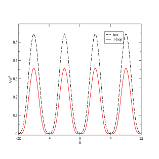
Figure 1: Periodic structure of the Little Higgs effective potential for $T=0$.

From the Lagrangian (14) we can extract the tree-level effective potential for the real scalar field $h\equiv\sqrt{2}{\mathrm{R}e}(H)$. In most previous papers an expansion in $h$ is performed. Here we avoid doing this, except to illustrate a few aspects, and keep the full dependence on $h$. The tree-level potential is a function of

$$\langle\Sigma\rangle=\exp\left[2i\langle\Pi\rangle/f\right]\Sigma_{0}=\left[I_{5}+i\sqrt{2}\frac{\langle\Pi\rangle}{h}\sin 2\alpha-4\frac{\langle\Pi\rangle^{2}}{h^{2}}\sin^{2}\alpha\right]\Sigma_{0}\ ,$$ (15)

where $\langle\Pi\rangle$ is only nonzero through $h$ and $\alpha\equiv h/(\sqrt{2}f)$. This is a periodic function and as a result the potential

$$V(h)={\mathrm{C}onstant}+f^{4}\left[2c{g^{\prime}}^{2}s_{\alpha}^{2}+{1\over 2}\lambda_{+}s_{\alpha}^{4}\right]\ ,$$ (16)

[where $\lambda_{\pm}\equiv c(g_{1}^{2}\pm g_{2}^{2})\pm 16c^{\prime}\lambda_{1}^{2}$] is invariant under $h\rightarrow h+n\pi f$. The minimum at the origin $h=0$ is replicated at $\pm n\pi f$ (see figure 1) with barriers of height $(2c{g^{\prime}}^{2}+\lambda_{+}/2)f^{4}$ separating these minima. In each of them, in spite of appearances (the fact that $h\neq 0$) the electroweak symmetry is unbroken. In fact one can show that the mass spectrum is the same in all these vacua, in particular SM gauge bosons are massless. In other words, the order parameter for electroweak symmetry breaking is $M_{W}$ rather than $\langle h\rangle$.

Regarding the local properties of these minima, an expansion in powers of $h$ around $h=0$ gives:

$$V(h)={\mathrm{C}onstant}+c{g^{\prime}}^{2}f^{2}h^{2}+{1\over 24}(3\lambda_{+}-4c{g^{\prime}}^{2})h^{4}+...$$ (17)

As expected, the only mass term for $h$ is due to the $U(1)_{Y}$ gauge coupling $g^{\prime}$. This offers an immediate possibility for electroweak symmetry breaking if one chooses $c<0$. In that case the minimum is at

$$\langle s_{\alpha}^{2}\rangle={-2c{g^{\prime}}^{2}\over\lambda_{+}}\ ,$$ (18)

or

$$\langle h^{2}\rangle\simeq{-12c{g^{\prime}}^{2}f^{2}\over(3\lambda_{+}-4c{g^{\prime}}^{2})}\ .$$ (19)

However, this tree-level breaking is problematic. The expansion of the potential to fourth order in $h$ and $t\equiv\sqrt{2}{\mathrm{R}e}(-i\phi)$ is:

$$V(h,t) = {\mathrm{C}onstant}+c{g^{\prime}}^{2}f^{2}h^{2}+{1\over 24}(3\lambda_{+}-4c{g^{\prime}}^{2})h^{4}+{1\over\sqrt{2}}\lambda_{-}fh^{2}t$$ (20)

$$+ (\lambda_{+}+4c{g^{\prime}}^{2})f^{2}t^{2}-{1\over 6}(4\lambda_{+}+17c{g^{\prime}}^{2})t^{2}h^{2}-{2\over 3}(\lambda_{+}+4c{g^{\prime}}^{2})t^{4}+...$$

In the presence of the coupling $\lambda_{-}$, a vev for $h$ induces a tadpole for $t$ so that the previous minimum gets slightly displaced. From (20) we get

$$\langle t\rangle\simeq{-\lambda_{-}f\over 2\sqrt{2}(\lambda_{+}+4c{g^{\prime}}^{2})}{\langle h^{2}\rangle\over f^{2}}\ ,$$ (21)

but one cannot obtain $|\lambda_{-}|\ll\lambda_{+}+4c{g^{\prime}}^{2}$ and as a result $\langle t\rangle$ turns out to be too large.

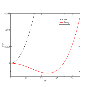
Figure 2: Close-up of fig. 1 to reveal the electroweak minimum.

Therefore the breaking has to be triggered by one-loop radiative corrections. In order to compute the one-loop potential, both at $T=0$ and at finite $T$, we need the mass spectrum in an arbitrary Higgs background $h$. This is easy to compute and one finds that the masses inherit the periodicity of $\langle\Sigma\rangle$ (we give the details in Appendix A). Then the one-loop potential is also a periodic function of $h$, as shown by figure 1, where it can be compared with the tree level one. In particular, the height of the barriers between minima is somewhat reduced. More importantly, the electroweak symmetry is now broken: the appearance of symmetry breaking minima is clearer in the close-up shown in figure 2. Analytically, this is understood as the result of the negative contribution from the heavy top to the Higgs mass. To order $h^{2}$ the $T=0$ one-loop potential reads

$$\delta_{1}V = {h^{2}\over 64\pi^{2}}\left[-12\lambda_{t}^{2}M_{T}^{2}\left(\log{\Lambda^{2}\over M_{T}^{2}}+1\right)+{9\over 2}g^{2}M_{W^{\prime}}^{2}\left(\log{\Lambda^{2}\over M_{W^{\prime}}^{2}}+{1\over 3}\right)\right.$$ (22)

$$\;\;\;\;\;\;\;\;\;\;\;+6\left(\lambda_{+}+5c{g^{\prime}}^{2}-{\lambda_{-}^{2}\over\lambda_{+}+3c{g^{\prime}}^{2}}\right)M^{2}_{1}\left(\log{\Lambda^{2}\over M^{2}_{1}}+1\right)$$

$$\;\;\;\;\;\;\;\;\;\;\;\left.+6\left(-\lambda_{+}+{5\over 3}c{g^{\prime}}^{2}+{\lambda_{-}^{2}\over\lambda_{+}+3c{g^{\prime}}^{2}}\right)M^{2}_{2}\left(\log{\Lambda^{2}\over M^{2}_{2}}+1\right)\right]+...,$$

where

$$M_{T}^{2} \equiv (\lambda_{1}^{2}+\lambda_{2}^{2})f^{2}\ ,$$ (23)

$$M_{W^{\prime}}^{2} \equiv {1\over 4}G_{+}^{2}f^{2}\ ,$$ (24)

$$M^{2}_{1} \equiv 2(\lambda_{+}+4c{g^{\prime}}^{2})f^{2}\ ,$$ (25)

$$M^{2}_{2} \equiv 2c{g^{\prime}}^{2}f^{2}\ .$$ (26)

We have chosen the following values for the parameters of the model: $\lambda_{1}=\lambda_{2}=1$, $g_{1}=g_{2}=\sqrt{2}g$, $\lambda_{+}=0.85$ and $\lambda_{-}=-0.0077$, so that $\langle h\rangle=246$ GeV for $f=1$ TeV. These parameters also give adequate values for the masses of the non SM particles in the model.

Before proceeding, it is convenient to say a word about our way of computing the masses of scalar fluctuations (i.e. the degrees of freedom in $\Sigma$ itself). In principle we could simply shift $h^{0}\rightarrow h^{0}+h/\sqrt{2}$ in $\Sigma$ to compute $h$-dependent scalar masses. To do this properly one should take into account that in general, after this shifting, the scalar kinetic terms from (11) are not canonical. Therefore one should rescale the fields to get the kinetic terms back to canonical form and this rescaling affects the ${\cal O}(h^{2})$ contributions to scalar masses. Instead of following this standard procedure we find it convenient to use an alternative method which simplifies the calculations and has appealing features when one is concerned about the global structure of the potential, see below.

The idea is to treat the new background with $\langle H\rangle=h/\sqrt{2}$ as a basis change (recall the discussion of the change from $\langle\Phi\rangle=I_{5}$ to $\langle\Phi\rangle=\Sigma_{0}$ in section 2). The $SU(5)$ transformation is now $U_{h}\equiv\exp(i\langle\Pi\rangle/f)$ with $\Sigma_{h}\equiv\langle\Sigma\rangle=U_{h}\Sigma_{0}U_{h}^{T}$. To parametrize the scalar fluctuations around this background we again use the exponentials of broken generators, but taking into account the effect of the change of basis, which acts on generators as $X_{a}\rightarrow U_{h}X_{a}U_{h}^{\dagger}$. That is, instead of using $\exp(i\Pi/f)$ we use $U_{h}\exp(i\Pi/f)U_{h}^{\dagger}$, and write for $\Sigma$:

$$\Sigma=(U_{h}e^{i\Pi/f}U_{h}^{\dagger})(U_{h}\Sigma_{0}U_{h}^{T})(U_{h}^{*}e^{i\Pi^{T}/f}U_{h}^{T})=e^{i\langle\Pi\rangle/f}e^{2i\Pi/f}e^{i\langle\Pi\rangle/f}\Sigma_{0}\ .$$ (27)

Alternatively, defining $\Pi_{N}=\pi_{a,N}X^{a,N}$ with $X_{a,N}=\exp(i\langle\Pi\rangle/f)X_{a}\exp(-i\langle\Pi\rangle^{T}/f)$ we have

$$\Sigma=e^{i\Pi_{N}/f}\Sigma_{h}e^{-i\Pi^{T}_{N}/f}=e^{2i\Pi_{N}/f}\Sigma_{h}\ .$$ (28)

[This parametrization allows the second equality of eq. (28) to hold as the condition $X_{a,N}\Sigma_{h}=\Sigma_{h}X_{a,N}^{T}$ is still valid.] The prescription in eq. (27) [or (28)] is to be compared with the standard procedure

$$\Sigma=e^{2i(\Pi+\langle\Pi\rangle)/f}\Sigma_{0}\ .$$ (29)

Some comments are in order. First, it is easy to check that with the prescription of eq. (27) scalar fluctuations are automatically canonical. Second, we are free to choose this parametrization of scalar fluctuations: a general theorem [15] guarantees that this different parametrization does not change the physics. Finally, using eq. (27) has another advantage when looking at global properties of the scalar potential. As mentioned above, the mass spectrum is the same in all the periodic degenerate minima of the potential. For the scalar sector this is trivial to show with our parametrization and a bit more cumbersome using the conventional parametrization of eq. (29) which, as explained, requires field redefinitions in order to recover canonical kinetic terms. Some of these field redefinitions are in fact singular (because some kinetic terms go to zero in these minima). Although the singularities cancel out when computing scalar masses (because some masses also go to zero in these minima) they can make some of the scalar couplings blow up. This can be interpreted as a failure of the parametrization (29) to cover the whole parameter space with a single coordinate patch. In this sense the parametrization (27) is to be preferred when discussing global properties of the scalar potential.

4 Effective Potential ($T$$\neq$$\mathrm{𝟎}$) and discussion

We calculate the finite temperature effective potential at one loop in order to study the dynamics of the scalar fields at finite temperature including the interactions with the thermal bath. To do this, we include the contributions from all particles that receive a correction to their mass from the vacuum expectation value of the nonlinear sigma model field $\langle\Sigma\rangle\equiv\Sigma_{h}$, just as we did for the one-loop potential at $T=0$. The one-loop thermal integrals for the contributions of bosonic and fermionic particles are standard, see e.g. [16]. For certain regions of $h$ some scalars might have negative masses squared, $m^{2}(h)<0$. For these we simply take the real part of the corresponding thermal integral.

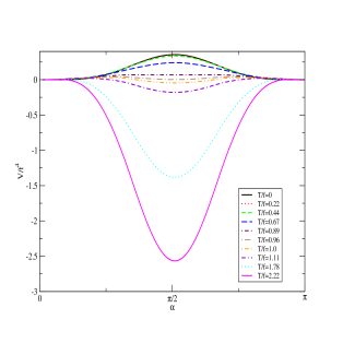
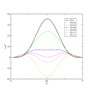
Figure 3: Evolution of the global structure of Higgs effective potential with temperature. The lower plot is a detail of the upper one, for a narrower range of temperatures around the critical temperature $T_{1}$.

Figure 3 shows the behaviour of the global structure of the potential for increasing values of the temperature. We see that the barrier between two minima decreases when $T$ is increased, eventually turning into a local minimum (where the electroweak symmetry is broken) that becomes the global minimum if $T$ is even higher. We can define a critical temperature $T_{1}$ at which this local minimum is degenerate with the minima at $h=0$. Numerically we obtain $T_{1}\simeq 0.96f$ for our particular choice of parameters ($T_{1}\sim f$ will be generic). An analysis of the thermal behaviour of models with pseudo-Goldstone bosons was done in [18], in a different context. We find that some of the generic features discussed in those papers resemble the behaviour we encounter for Little Higgs models.

In order to understand analytically the particular behaviour of the potential shown in figure 3 it is enough to consider the case of $T\stackrel{{\scriptstyle>}}{{{}_{\sim}}}f$. At such high $T$ (still below $\Lambda$) an expansion in powers of $m/T$ gives a good approximation to the potential. Writing also the one-loop $T=0$ part, one obtains in general

$$\delta_{1}V \simeq {T^{2}\over 24}\left({\mathrm{T}r}M_{B}^{2}+{1\over 2}{\mathrm{T}r}M_{F}^{2}\right)-{T\over 12\pi}{\mathrm{T}r}M_{B}^{3}$$ (30)

$$+ {1\over 64\pi^{2}}\left[{\mathrm{T}r}M_{B}^{4}\left(\log{c_{B}T^{2}\over\Lambda^{2}}+\kappa_{B}\right)-{\mathrm{T}r}M_{F}^{4}\left(\log{c_{F}T^{2}\over\Lambda^{2}}+\kappa_{F}\right)\right]\ ,$$

where $B=\{S,V\}$ labels bosonic degrees of freedom (scalar and vector bosons) and $F$ fermionic ones. The constants $\kappa_{B,F}$ come from the one-loop $T=0$ potential and are simply $\kappa_{S}=\kappa_{F}=-3/2$ and $\kappa_{V}=-5/6$ while $c_{B,F}$ come instead from the finite temperature part and are $\log c_{B}\simeq 5.41$ and $\log c_{F}\simeq 2.64$. Keeping only the dominant $T^{2}$ term we get for our model (see appendix A):

$$\delta_{T}V=-{1\over 24}f^{2}T^{2}\left\{\left[12\lambda_{+}+\lambda_{1}^{2}(64c^{\prime}+6)-{3\over 8}(g_{1}^{2}+g_{2}^{2})\right]s_{\alpha}^{4}+{g^{\prime}}^{2}\left[48c-{3\over 2}\right]s_{\alpha}^{2}\ \right\}\ .$$ (31)

First we see that expanding around $h=0$, the thermal mass is proportional to $g^{\prime}$, as expected on general grounds. For the range of temperatures we are considering, this thermal effect is not strong enough to produce a minimum in $h=0$, the one-loop $T=0$ corrections dominate and indeed the potential at $h=0$ has a maximum. Next we examine larger values of $h$. In eq. (31) the gauge contribution is subdominant, and the scalar and fermionic terms provide a deep minimum for the potential at the intermediate point $\alpha=\pi/2$. This is precisely the high $T$ behaviour that we find in figure 3.

The results indicating symmetry nonrestoration of the gauge electroweak symmetry directly lead us to pose the question of what could be the associated cosmology. As we have said already, we are restricted by our analysis to temperatures beneath $\Lambda/\pi\simeq 4f$. Suppose now that we follow the behaviour of the system starting from low temperatures and heating up the thermal bath. As one can infer from the lower plot of Fig. 3, the electroweak gauge symmetry is restored at some temperature $T_{\rm ew}$ of the order of the electroweak scale. This means that $h=0$ (modulo $\pi f$) becomes the ground state of the system. This is completely analogous to what happens in the SM. However, a further increase of the temperature results in a decrease of the height of the barrier between the periodic minima at $h=0,\pi f,...$. For even larger values of the temperature beyond $T_{1}\sim f$, the maximum at $h=\pi f/2$ (modulo $\pi f$) turns into the global minimum and the barrier among the new equivalent vacua increases with temperature.

The cosmology of the Little Higgs model will therefore depend strongly on the maximum temperature that the Universe has attained after a period of inflation [19], which is necessary to explain the homogeneity and the isotropy of our observed Universe. Suppose that such a temperature is smaller than $T_{1}$ and that the minima at $h=0,\pi f,...$ are always the ground state until the electroweak phase transition. If so, the situation is completely analogous to the SM. Suppose, however, that the highest temperature after inflation is indeed larger than $T_{1}$. Under these circumstances, the Universe is characterized by a high temperature phase during which the electroweak symmetry is broken. This period will last till the temperature drops somewhat below $T_{1}$ at which point there will be a phase transition to the symmetric phase (followed later on by the usual SM electroweak phase transition back to the broken phase). This prediction is completely different from what is obtained in the SM. It would be very interesting to analyze the role played by this non-standard phase of broken symmetry in the evolution of the early Universe, e.g. on the possible baryon asymmetry production [20].

In view of the small thermal mass that comes from (31) (which is even zero in most Little Higgs models), one might wonder if two-loop $T\neq 0$ effects can then become important. In fact, at $T=0$, two-loop quadratically divergent corrections to the Higgs mass parameter go as $\delta m^{2}\sim\Lambda^{2}/(16\pi^{2})^{2}\sim f^{2}/(16\pi^{2})$, the same order as one-loop non-divergent contributions. (We did not include them because the one-loop contributions will in principle dominate due to logarithmic enhancement). At $T\neq 0$ one would correspondingly expect corrections of order $\delta m_{eff}^{2}\sim T^{2}/(16\pi^{2})$, which may be important precisely when the one loop thermal mass is suppressed (or absent). In fact, as the $T=0$ Higgs mass squared is itself of order $f^{2}/(16\pi^{2})$, a two-loop thermal mass of that order can be relevant when $T\stackrel{{\scriptstyle>}}{{{}_{\sim}}}f$. A complete two-loop calculation of the finite $T$ effective potential is beyond the scope of this paper, but it is of interest and we plan to undertake it in a future analysis. At this point we simply make two remarks. The first is that, for values of $h$ away from the origin, the one-loop $T^{2}$ contribution to the potential [eq. (31)] is negative and not suppressed. Therefore, the potential in that region will not change much after including two-loop corrections, which will be sub-dominant there. This gives us confidence on the inverse symmetry breaking behaviour we have found. The second remark is that we see no reason to expect that the two-loop contributions to the Higgs thermal mass will be positive. If they are, the details of the transition around $T_{1}$ will change (but not the existence of the transition itself) while if they are negative, our conclusions would be even stronger.

Let us close this section by a couple of comments. First, a complete study of the scalar potential should also include the temperature evolution of the triplet vev. For that purpose the spectrum in a more general background with nonzero $h$ and $t$ is needed. This complicates significantly the analysis, especially if one insists on keeping the $h$ and $t$ dependence to all orders (the potential is also periodic along the $t$ direction). We nevertheless performed such analysis and some of our results are presented in appendix B. Schematically, the potential has an egg-crate structure with different barrier heights for each direction. Although the potential at finite temperature along the $t$ direction can behave quite differently, depending on the choice of parameters, from what we described for the $h$ direction we find it interesting at present to focus on the Higgs direction alone.

Secondly, the previous analysis has assumed that $f$ is a constant, independent of temperature. However, we know that $f$ is in fact the vev of $\Sigma$ (along a particular direction), producing the breaking $SU(5)\rightarrow SO(5)$. As such it is a dynamical variable and it is expected that at sufficiently high $T$ one will get $f\rightarrow 0$, corresponding to a critical temperature $T_{*}$ for the $SU(5)\rightarrow SO(5)$ transition. As we do not know what is the physics beyond the cutoff scale $\Lambda$, where the dynamics of the system is superseded by the UV completion of the theory, we do not know the potential that produced the vev $f$ in the first place. Therefore, it is difficult to be precise about $T_{*}$. However we can make an estimate of the temperature behaviour of $f$ (in the spirit of [17] for the more complicated case of the chiral condensate in QCD). We can just approximate the zero temperature potential for $f$ by a Mexican hat potential

$$V(f)=\kappa^{2}(f^{2}-\langle f\rangle^{2})^{2}\ ,$$ (32)

where $\kappa$ is some unknown constant and $\langle f\rangle$ is assumed to be $\sim 1$ TeV (it corresponds to the $f$ used in the rest of the paper). We then add to the potential (32) the finite temperature corrections coming from all the particles that have an $f$-dependent mass. These are listed in eqs. (24)-(26). The value of $\kappa$ in eq. (32) is now crucial to the change of $f$ with increasing $T$. We argue that a natural choice is $\kappa\sim 2\pi$, because fluctuations around the minimum of the potential (32) along the $f$ direction have mass $2\kappa\langle f\rangle$ and we are assuming that the only scalar fields below the cutoff scale $\Lambda=4\pi\langle f\rangle$ are those contained in $\Pi$. Therefore we should demand $2\kappa\langle f\rangle\stackrel{{\scriptstyle>}}{{{}_{\sim}}}\Lambda$ which indeed translates into $\kappa\stackrel{{\scriptstyle>}}{{{}_{\sim}}}2\pi$. Choosing then that value of $\kappa$ for the numerical evaluation of the effective potential for $f$, we find that $f$ changes very little with $T$. For the extreme value $T=4\langle f\rangle$ we obtain $f(T)\simeq 0.9f$, just a $10\%$ decrease.

5 Conclusions

We have shown, on very general grounds, that the behaviour of Little Higgs models at finite temperature is considerably richer than in the Standard Model. In particular we have studied the effective potential at finite temperature which, as the Higgs $h$ in these models is a pseudo-Goldstone boson, is a periodic function of $h$.

Although the electroweak phase transition is expected to occur just like in the Standard Model, at higher temperatures, when the new states introduced in Little Higgs models at a scale $f\sim 1$ TeV are thermally produced in the plasma, the history of the early Universe changes dramatically. At some temperature $T_{1}\sim f$ a new minimum where the electroweak symmetry is broken becomes the global minimum of the potential and the gauge electroweak symmetry becomes more and more broken as the temperature continues to increase. Being a perturbative statement, it would be interesting to see if such a behaviour persists when non-perturbative corrections are accounted for, or what is the fate of this broken minimum in the context of the UV completion of the theory. At any rate, this rich structure at high temperatures might have cosmological implications which are worth studying.

As a spin-off, we have introduced a new parametrization of scalar fluctuations around displaced vacua in nonlinear sigma models which has very appealing features and might be of interest for phenomenological studies.

A. Spectrum of the Little Higgs model

In this appendix we present the mass matrices in a Higgs background for the Little Higgs model [10] studied in this paper. These masses are needed in the calculation of the one-loop Higgs potential, both at zero and finite temperature. We keep the exact dependence on the Higgs background $\langle h^{0}\rangle=h/\sqrt{2}$ so that we can study the global structure of the potential. We also present the mass eigenvalues in an expansion up to $h^{2}$. The scalar sector contains a complex $SU(2)$ triplet, a real triplet, the Higgs doublet and a singlet, a total of 14 degrees of freedom that are distributed in one doubly charged scalar, three charged fields and 6 neutral and real fields (4 CP odd and 2 CP even). The gauge boson sector contains a heavy $W^{\prime}$ and a heavy $Z^{\prime}$ besides the SM gauge bosons. The fermion sector of relevance for our calculation contains a heavy top in addition to the SM top quark. We follow the notation introduced in section 2. We remind the reader here that $\lambda_{+}\equiv c\,G_{+}^{2}+16c^{\prime}\lambda_{1}^{2}$ and $\lambda_{-}\equiv c\,G_{-}^{2}-16c^{\prime}\lambda_{1}^{2}$, with $G_{+}^{2}\equiv g_{1}^{2}+g_{2}^{2}$, $G_{-}^{2}\equiv g_{1}^{2}-g_{2}^{2}$. We also use $\alpha\equiv h/(\sqrt{2}f)$, where $h$ is normalized as a real field. (At $T=0$ one has $\langle h\rangle=246$ GeV.) The mass matrices presented below correspond to canonically normalized fields (see section 3 for a discussion on this point for the scalar sector). The mass eigenvalues of all scalar fields are periodic under $\alpha\rightarrow\alpha+\pi$.

Doubly charged scalar

The field $\phi^{++}$ has a mass

$$M_{\phi^{++}}^{2}=2f^{2}(\lambda_{+}+4c{g^{\prime}}^{2}-16c^{\prime}\lambda_{1}^{2}s^{4}_{\alpha})=2(\lambda_{+}+4c{g^{\prime}}^{2})f^{2}+{\cal O}(h^{4}/f^{2})\ .$$ (A.1)

At order $h^{2}$ this state does not contribute to the trace of the mass squared operator.

Charged scalars

In the basis $\{\xi^{+},\phi^{+},h^{+}\}$, the mass matrix $M_{+}^{2}$ for the charged scalars $\varphi_{i}^{+}$ is

$$M^{2}_{+} = f^{2}\left[\begin{array}[]{ccc}-2\lambda_{+}c_{\alpha}(2+c_{\alpha})s^{4}_{\alpha/2}&{1\over 2}\lambda_{+}c_{\alpha}^{2}s^{2}_{\alpha}&-{i\over\sqrt{2}}\lambda_{-}s_{2\alpha}s^{2}_{\alpha/2}\\ &&\\ {1\over 2}\lambda_{+}c_{\alpha}^{2}s^{2}_{\alpha}&2\lambda_{+}c_{\alpha}(2-c_{\alpha})c^{4}_{\alpha/2}&-{i\over\sqrt{2}}\lambda_{-}s_{2\alpha}c^{2}_{\alpha/2}\\ &&\\ {i\over\sqrt{2}}\lambda_{-}s_{2\alpha}s^{2}_{\alpha/2}&{i\over\sqrt{2}}\lambda_{-}s_{2\alpha}c^{2}_{\alpha/2}&\lambda_{+}s^{2}_{\alpha}c^{2}_{\alpha}\end{array}\right]$$ (A.7)

$$+ c{g^{\prime}}^{2}f^{2}\left[\begin{array}[]{ccc}2(1-3c_{\alpha})s^{2}_{\alpha/2}&s^{2}_{\alpha}&0\\ s^{2}_{\alpha}&2(1+3c_{\alpha})c^{2}_{\alpha/2}&0\\ 0&0&2c^{2}_{\alpha}\end{array}\right]\ .$$ (A.11)

For the trace we obtain

$$2{\mathrm{T}r}M^{2}_{+}=4\lambda_{+}f^{2}(1-s^{4}_{\alpha})+4c{g^{\prime}}^{2}f^{2}(5-4s^{2}_{\alpha})\ ,$$ (A.12)

and an expansion in powers of $h$ gives

$$2{\mathrm{T}r}M^{2}_{+}={\mathrm{C}onstant}-8c{g^{\prime}}^{2}h^{2}+{\cal O}(h^{4}/f^{2})\ ,$$ (A.13)

with the only contribution to order $h^{2}$ being that of the $U(1)_{Y}$ sector. A similar expansion for the mass eigenvalues gives

$$m^{2}_{\varphi_{1}^{+}} = -{1\over 2}c{g^{\prime}}^{2}h^{2}+...$$ (A.14)

$$m^{2}_{\varphi_{2}^{+}} = 2(\lambda_{+}+4c{g^{\prime}}^{2})f^{2}-{1\over 2}\left[\lambda_{+}+5c{g^{\prime}}^{2}-{\lambda_{-}^{2}\over\lambda_{+}+3c{g^{\prime}}^{2}}\right]h^{2}+...$$ (A.15)

$$m^{2}_{\varphi_{3}^{+}} = 2c{g^{\prime}}^{2}f^{2}+{1\over 2}\left[\lambda_{+}-2c{g^{\prime}}^{2}-{\lambda_{-}^{2}\over\lambda_{+}+3c{g^{\prime}}^{2}}\right]h^{2}+...$$ (A.16)

For $h=0$, $\varphi_{1}^{+}=\xi^{+}$ is the charged Goldstone boson associated to the gauge symmetry breaking $SU(2)_{1}\times SU(2)_{2}\rightarrow SU(2)_{SM}$ and we get $m^{2}_{\varphi_{1}^{+}}=0$.

Neutral scalars

For the neutral scalar fields $\varphi_{i}^{0}$ we use the basis $\{\zeta^{0},\xi^{0},\phi^{0r},\phi^{0i},h^{0r},h^{0i}\}$, where we have decomposed the complex fields $\phi^{0}$ and $h^{0}$ as $h^{0}=(h^{0r}+ih^{0i})/\sqrt{2}$ and $\phi^{0}=i(\phi^{0r}+i\phi^{0i})/\sqrt{2}$. The mass matrix for neutral scalar fields, $M_{0}^{2}$, breaks up in two blocks: one for the pseudoscalars $\{\zeta^{0},\xi^{0},\phi^{0i},h^{0i}\}$ and the other for the scalars $\{\phi^{0r},h^{0r}\}$. The $4\times 4$ block is

$$M^{2}_{4\times 4} = -{1\over 4}f^{2}\left[\begin{array}[]{cccc}5\lambda_{+}s_{\alpha}^{4}&\sqrt{5}\lambda_{+}s_{\alpha}^{4}&\sqrt{10}\lambda_{+}(2-s_{\alpha}^{2})s^{2}_{\alpha}&0\\ \sqrt{5}\lambda_{+}s_{\alpha}^{4}&\lambda_{+}s_{\alpha}^{4}&\sqrt{2}\lambda_{+}(2-s_{\alpha}^{2})s^{2}_{\alpha}&0\\ \sqrt{10}\lambda_{+}(2-s_{\alpha}^{2})s^{2}_{\alpha}&\sqrt{2}\lambda_{+}(2-s_{\alpha}^{2})s^{2}_{\alpha}&-2\lambda_{+}(4c_{\alpha}^{2}-s^{4}_{\alpha})&4\lambda_{-}c_{\alpha}s_{2\alpha}\\ 0&0&4\lambda_{-}c_{\alpha}s_{2\alpha}&-\lambda_{+}s^{2}_{2\alpha}\end{array}\right]$$ (A.21)

$$- c{g^{\prime}}^{2}f^{2}\left[\begin{array}[]{cccc}5s_{\alpha}^{2}&\sqrt{5}s_{\alpha}^{2}&\sqrt{10}s^{2}_{\alpha}&0\\ \sqrt{5}s_{\alpha}^{2}&s_{\alpha}^{2}&\sqrt{2}s^{2}_{\alpha}&0\\ \sqrt{10}s^{2}_{\alpha}&\sqrt{2}s^{2}_{\alpha}&-2(4-5s^{2}_{\alpha})&0\\ 0&0&0&-2c^{2}_{\alpha}\end{array}\right]\ ,$$ (A.26)

which has a zero eigenvalue, corresponding to the eigenvector $(1,-\sqrt{5},0,0)/\sqrt{6}$ [the neutral Goldstone boson associated to the breaking of an ungauged $U(1)$].

The $2\times 2$ block is:

$$M_{2\times 2}^{2}=f^{2}\left[\begin{array}[]{cc}\lambda_{+}(2c_{\alpha}^{2}-s_{\alpha}^{4})&\lambda_{-}(3s_{\alpha}^{2}-2)s_{\alpha}\\ \lambda_{-}(3s_{\alpha}^{2}-2)s_{\alpha}&\lambda_{+}(3-4s_{\alpha}^{2})s_{\alpha}^{2}\end{array}\right]+2c{g^{\prime}}^{2}f^{2}\left[\begin{array}[]{cc}4-5s_{\alpha}^{2}&0\\ 0&c_{2\alpha}\end{array}\right]\ .$$ (A.27)

From these matrices we obtain

$${\mathrm{T}r}M^{2}=4\lambda_{+}f^{2}(1-2s^{4}_{\alpha})+4c{g^{\prime}}^{2}f^{2}(5-8s^{2}_{\alpha})\ .$$ (A.28)

An expansion in powers of $h$ gives

$${\mathrm{T}r}M^{2}={\mathrm{C}onstant}-16c{g^{\prime}}^{2}h^{2}+{\cal O}(h^{4}/f^{2})\ ,$$ (A.29)

with the only contribution of order $h^{2}$ being that of the $U(1)_{Y}$ sector. The expansion of the mass eigenvalues gives, for the $4\times 4$ block:

$$m^{2}_{\varphi_{1}^{0}} = 0$$ (A.30)

$$m^{2}_{\varphi_{2}^{0}} = -3c{g^{\prime}}^{2}h^{2}+...$$ (A.31)

$$m^{2}_{\varphi_{3}^{0}} = 2(\lambda_{+}+4c{g^{\prime}}^{2})f^{2}-\left[\lambda_{+}+5c{g^{\prime}}^{2}-{\lambda_{-}^{2}\over\lambda_{+}+3c{g^{\prime}}^{2}}\right]h^{2}+...$$ (A.32)

$$m^{2}_{\varphi_{4}^{0}} = 2c{g^{\prime}}^{2}f^{2}+{1\over 2}\left[\lambda_{+}-2c{g^{\prime}}^{2}-{2\lambda_{-}^{2}\over\lambda_{+}+3c{g^{\prime}}^{2}}\right]h^{2}+...$$ (A.33)

while for the $2\times 2$ block we get

$$m^{2}_{\varphi_{5}^{0}} = 2(\lambda_{+}+4c{g^{\prime}}^{2})f^{2}-\left[\lambda_{+}+5c{g^{\prime}}^{2}-{\lambda_{-}^{2}\over\lambda_{+}+3c{g^{\prime}}^{2}}\right]h^{2}+...$$ (A.34)

$$m^{2}_{\varphi_{6}^{0}} = 2c{g^{\prime}}^{2}f^{2}+{1\over 2}\left[3\lambda_{+}-4c{g^{\prime}}^{2}-{2\lambda_{-}^{2}\over\lambda_{+}+3c{g^{\prime}}^{2}}\right]h^{2}+...$$ (A.35)

For $h=0$ we have two zero mass eigenvalues: the Goldstones $\xi^{0}$ and $\zeta^{0}$.

Gauge Bosons

The mass matrix for the charged gauge bosons ($W^{\pm},{W^{\prime}}^{\pm}$) in the interaction basis is given by

$$M_{W}^{2}={f^{2}\over 4}\left[\begin{array}[]{cc}g_{1}^{2}&-g_{1}g_{2}c^{2}_{\alpha}\\ -g_{1}g_{2}c^{2}_{\alpha}&g_{2}^{2}\end{array}\right]\ ,$$ (A.36)

which has periodic mass eigenvalues.

There are three neutral gauge bosons: $Z^{0}$, ${Z^{\prime}}^{0}$ and the photon. Their $3\times 3$ mass matrix in the interaction basis is

$$M_{Z,A}^{2}={f^{2}\over 8}\left[\begin{array}[]{ccc}g_{1}^{2}(2+s^{4}_{\alpha})&-g_{1}g_{2}(1+c^{4}_{\alpha})&2g_{1}g^{\prime}s^{2}_{\alpha}\\ -g_{1}g_{2}(1+c^{4}_{\alpha})&g_{2}^{2}(2+s^{4}_{\alpha})&2g_{2}g^{\prime}s^{2}_{\alpha}\\ 2g_{1}g^{\prime}s^{2}_{\alpha}&2g_{2}g^{\prime}s^{2}_{\alpha}&4{g^{\prime}}^{2}s^{2}_{\alpha}\end{array}\right]\ ,$$ (A.37)

again with periodic eigenvalues. It can be easily checked that $M_{Z,A}^{2}$ annihilates the vector $(1/g_{1},1/g_{2},-1/g^{\prime})$, which corresponds to the photon. For the trace of $M^{2}$ we get

$${\mathrm{T}r}M_{V}^{2}=2{\mathrm{T}r}M_{W}^{2}+{\mathrm{T}r}M_{Z,A}^{2}={1\over 8}G_{+}^{2}f^{2}(6+s_{\alpha}^{4})+{1\over 2}{g^{\prime}}^{2}f^{2}s_{\alpha}^{2}\ ,$$ (A.38)

and expanding in powers of $h$,

$${\mathrm{T}r}M_{V}^{2}={\mathrm{C}onstant}+{1\over 4}{g^{\prime}}^{2}h^{2}+{\cal O}(h^{4}/f^{2})\ .$$ (A.39)

The expansion of the mass eigenvalues is

$$m^{2}_{W^{\pm}} = {1\over 4}g^{2}h^{2}+...$$ (A.40)

$$m^{2}_{{W^{\prime}}^{\pm}} = {1\over 4}G_{+}^{2}f^{2}-{1\over 4}g^{2}h^{2}...$$ (A.41)

$$m^{2}_{Z^{0}} = {1\over 4}(g^{2}+{g^{\prime}}^{2})h^{2}+...$$ (A.42)

$$m^{2}_{{Z^{\prime}}^{0}} = {1\over 4}G_{+}^{2}f^{2}-{1\over 4}g^{2}h^{2}...$$ (A.43)

where we have used $g^{2}\equiv g_{1}^{2}g_{2}^{2}/(g_{1}^{2}+g_{2}^{2})$.

Fermions

For the top quark and its heavy partner we have

$$M_{f}M_{f}^{\dagger}=f^{2}\left(\begin{array}[]{cc}\lambda_{2}^{2}&\lambda_{1}\lambda_{2}c^{2}_{\alpha}\\ \lambda_{1}\lambda_{2}c^{2}_{\alpha}&\lambda_{1}^{2}(1-s^{4}_{\alpha})\end{array}\right)\ ,$$ (A.44)

which has periodic eigenvalues. The fermionic trace is

$${\mathrm{T}r}(M_{f}M_{f}^{\dagger})=f^{2}\left[\lambda_{2}^{2}+\lambda_{1}^{2}(1-s_{\alpha}^{4})\right]\ ,$$ (A.45)

which does not contribute to order $h^{2}$. The expansion of the two mass eigenvalues can be written as

$$m^{2}_{t} = {1\over 2}\lambda_{t}^{2}h^{2}+...$$ (A.46)

$$m^{2}_{T} = (\lambda_{1}^{2}+\lambda_{2}^{2})f^{2}-{1\over 2}\lambda_{t}^{2}h^{2}...$$ (A.47)

where the top Yukawa is given by $\lambda_{t}^{2}\equiv 2\lambda_{1}^{2}\lambda_{2}^{2}/(\lambda_{1}^{2}+\lambda_{2}^{2})$.

B. The triplet direction

As mentioned in the main text, in this model a nonzero vacuum expectation value of $\langle h^{0}\rangle=h/\sqrt{2}$ will induce a vev for the triplet field $\langle\phi_{0}^{r}\rangle=t/\sqrt{2}$. The tree-level potential to all orders in $h$ and $t$ is given by,

$$V_{0} = \frac{\lambda_{+}f^{4}}{(t^{2}+h^{2})^{2}}\left[3(t^{2}+h^{2})^{2}+\frac{1}{2}t^{2}(t^{2}+h^{2})s^{2}_{2\beta}+\frac{1}{2}h^{4}s^{4}_{\beta}\right]$$ (B.1)

$$- \frac{\lambda_{-}f^{4}}{(t^{2}+h^{2})^{2}}th^{2}(t^{2}+h^{2})^{1/2}s^{2}_{\beta}s_{2\beta}+\frac{2cf^{4}g^{\prime 2}}{(t^{2}+h^{2})}\left[t^{2}s^{2}_{2\beta}+h^{2}s^{2}_{\beta}\right]\ ,$$

where $\beta=(t^{2}+h^{2})^{1/2}/(\sqrt{2}f)$. We see that the potential is periodic along the $t$-direction as well.

A complete analysis of the one-loop corrections to the potential (B.1), both at $T=0$ and $T\neq 0$ requires the calculation of the mass matrices of all particles in the presence of the background fields $h,t$, which is not an easy task, although we did perform it. The generic expressions one obtains for these mass matrices are too long and complicated to be given here.

In this paper we limit ourselves to give an example of the kind of dynamics one might obtain along the triplet direction. The interest of this is not limited by the fact that the phenomenological complications associated to the presence of a triplet vacuum expectation value can be neatly solved by imposing a $T$-parity on the model [11]. As we will explain next, even if one does not have a tadpole for $t$ the triplet direction might play a role in the thermal evolution of the Universe.

The argument that leads one to expect a peculiar behaviour of the effective potential at finite temperature along the Higgs doublet direction (namely the fact that quadratically divergent corrections to the Higgs mass vanish) does not hold for the triplet direction. Explicitly, an expansion of the $t$-dependent masses for the gauge bosons along the triplet direction gives

$$m^{2}_{W^{\pm}} = {1\over 2}g^{2}t^{2}+...$$ (B.2)

$$m^{2}_{{W^{\prime}}^{\pm}} = {1\over 4}G_{+}^{2}f^{2}-{1\over 2}g^{2}t^{2}...$$ (B.3)

$$m^{2}_{Z^{0}} = (g^{2}+{g^{\prime}}^{2})t^{2}+...$$ (B.4)

$$m^{2}_{{Z^{\prime}}^{0}} = {1\over 4}G_{+}^{2}f^{2}+{1\over 4}{G_{-}^{4}\over G_{+}^{2}}t^{2}...$$ (B.5)

so that the trace is

$$3{\mathrm{T}r}M_{V}^{2}={\mathrm{C}onstant}+{3\over 4}(G_{+}^{2}+4{g^{\prime}}^{2})t^{2}+...$$ (B.6)

For fermions one gets

$$12{\mathrm{T}r}M_{F}^{2}={\mathrm{C}onstant}-24\lambda_{1}^{2}t^{2}+...,$$ (B.7)

while for scalars

$${\mathrm{T}r}M_{S}^{2}={\mathrm{C}onstant}-{4\over 5}(318c{g^{\prime}}^{2}+1488c^{\prime}\lambda_{1}^{2}+49\lambda_{+})t^{2}+...$$ (B.8)

These results determine that the thermal potential along the triplet direction has a $T^{2}$ contribution

$$\delta V(T) = -{1\over 2}\kappa_{t}^{2}t^{2}T^{2}$$ (B.9)

$$= {1\over 48}\left[{3\over 2}(G_{+}^{2}+4{g^{\prime}}^{2})-{8\over 5}(318c{g^{\prime}}^{2}+1488c^{\prime}\lambda_{1}^{2}+49\lambda_{+})-24\lambda_{1}^{2}\right]t^{2}T^{2}\ .$$

The negative contributions to the traces in (B.7) and (B.8) dominate in the potential (B.9), making $\kappa_{t}^{2}>0$. This unusual behaviour implies that for temperatures above a critical value

$$T_{t}^{c}=M_{t}/\kappa_{t}\ ,$$ (B.10)

where $M_{t}^{2}=2(\lambda_{+}+4c{g^{\prime}}^{2})f^{2}$ is the triplet mass squared, the electroweak symmetry gets broken along the triplet direction. That is, even if a $T$-parity forbids a tadpole $h^{2}t$ in the potential, and even if the mass of the triplet is large (of order $f$), thermal corrections will trigger electroweak symmetry breaking along the triplet direction, for some $T_{t}^{c}\sim f$. Of course one can increase the value of $T_{t}^{c}$ by appropriately choosing the parameters of the model and in this spirit we have not discussed this transition in the main text, and have focused instead in the Higgs direction. Nevertheless, this makes the possible structure of phase transitions in these models even richer.

References

- [1] N. Arkani-Hamed, A. G. Cohen and H. Georgi, Phys. Lett. B 513 (2001) 232 [hep-ph/0105239]; N. Arkani-Hamed, A. G. Cohen, T. Gregoire and J. G. Wacker, JHEP 0208 (2002) 020 [hep-ph/0202089]; N. Arkani-Hamed, A. G. Cohen, E. Katz, A. E. Nelson, T. Gregoire and J. G. Wacker, JHEP 0208 (2002) 021 [hep-ph/0206020].
- [2] N. Arkani-Hamed, A. G. Cohen, E. Katz and A. E. Nelson, JHEP 0207 (2002) 034 [hep-ph/0206021].
- [3] M. Schmaltz, Nucl. Phys. Proc. Suppl. 117 (2003) 40 [hep-ph/0210415]; D. E. Kaplan and M. Schmaltz, JHEP 0310 (2003) 039 [hep-ph/0302049].
- [4] J. G. Wacker, [hep-ph/0208235].
- [5] T. Han, H. E. Logan, B. McElrath and L. T. Wang, Phys. Rev. D 67 (2003) 095004 [hep-ph/0301040].
- [6] C. Csaki, J. Hubisz, G. D. Kribs, P. Meade and J. Terning, Phys. Rev. D 67 (2003) 115002 [hep-ph/0211124]; Phys. Rev. D 68 (2003) 035009 [hep-ph/0303236].
- [7] J. L. Hewett, F. J. Petriello and T. G. Rizzo, JHEP 0310 (2003) 062 [hep-ph/0211218].
- [8] G. Burdman, M. Perelstein and A. Pierce, Phys. Rev. Lett. 90, 241802 (2003) [Erratum-ibid. 92, 049903 (2004)] [hep-ph/0212228].
- [9] M. C. Chen and S. Dawson, Phys. Rev. D 70 (2004) 015003 [hep-ph/0311032].
- [10] M. Perelstein, M. E. Peskin and A. Pierce, Phys. Rev. D 69, 075002 (2004) [hep-ph/0310039].
- [11] H. C. Cheng and I. Low, [hep-ph/0405243]; JHEP 0309 (2003) 051 [hep-ph/0308199].
- [12] D. A. Kirzhnits, JETP Lett. 15 (1972) 529 [Pisma Zh. Eksp. Teor. Fiz. 15 (1972) 745]; D. A. Kirzhnits and A. D. Linde, Phys. Lett. B 42 (1972) 471.
- [13] D. Comelli and J. R. Espinosa, Phys. Rev. D 55, 6253 (1997) [hep-ph/9606438].
- [14] J. Orloff, Phys. Lett. B 403 (1997) 309 [hep-ph/9611398].
- [15] S. Kamefuchi, L. O’Raifeartaigh and A. Salam, Nucl. Phys. 28, 529 (1961).
- [16] G. W. Anderson and L. J. Hall, Phys. Rev. D 45 (1992) 2685.
- [17] C. Wetterich, Phys. Rev. D 66, 056003 (2002) [hep-ph/0102044].
- [18] A. K. Gupta, C. T. Hill, R. Holman and E. W. Kolb, Phys. Rev. D 45, 441 (1992); R. Holman and A. Singh, Phys. Rev. D 47 (1993) 421.
- [19] D. H. Lyth and A. Riotto, Phys. Rept. 314, 1 (1999) [hep-ph/9807278].
- [20] A. Riotto and M. Trodden, Ann. Rev. Nucl. Part. Sci. 49, 35 (1999) [hep-ph/9901362].