Chiral Meson Physics at Two Loops

Abstract

An overview of Chiral Perturbation Theory calculations in the mesonic sector at the two Loop level is given. Discussed in some detail are the partially quenched case relevant for lattice QCD, the general fitting procedures and $\pi\pi$,$\pi K$ scattering as well as the determination of $V_{us}$ and $K_{\ell 3}$ decays.

2 Introduction

In this meeting we have talked mainly about nuclei and baryons but I will concentrate on mesons. The reason is that the lightest mesons are the simplest bound states present in Quantum Chromo Dynamics (QCD). They have the minimal number of constituents and are the lightest state so should be spatially the simplest. Their properties are to a large extent determined by Chiral Symmetry which enforces vanishing masses in the limit of zero current quark masses, the chiral limit, as well as vanishing interactions in the zero momentum and chiral limit. It is the combination of these two properties that allows us to produce a well defined low energy theory, Chiral Perturbation Theory (ChPT), as a consistent approximation to QCD. In the remainder I review ChPT at two loops.

2.1 (Effective) Field Theory, ChPT and lattice QCD

The underlying idea is really the essence of (most of) physics. Use the right degrees of freedom. When there is a gap in the spectrum with a consequent separation of scales, we can build the theory containing only the lighter degrees of freedom and include the effects of the neglected high mass/energy states perturbatively by building the most general (local) Lagrangian with the low mass degrees of freedom. This leads in general to an infinite number of parameters so no predictivity is left. But when these terms can be ordered in importance by some principle, usually referred to as power counting, we have a finite number of parameters at any given order and thus an effective theory.

We need to use field theory since it is the only known way to locally combine quantum mechanics and special relativity. A Taylor expansion cannot be used because in the chiral limit the continuum of states gives it zero convergence radius. As important is the fact that off-shell effects are fully under control. The freedom allowed by this is fully described by extra free parameters. In addition it is systematic, all effects at a given order in the expansion are included and errors can be estimated. Drawbacks are of course the large number of free parameters, but do not forget the fact that while a model can have few parameters there is a large freedom in the space of possible models hidden behind it, and as always the expansion itself might also not converge.

For ChPT the included degrees of freedom are the Goldstone Bosons from spontaneous breakdown of chiral symmetry, identified with the pseudoscalar octet, $\pi^{\pm,0}$, $K^{\pm}$,$K^{0}$, $\overline{K^{0}}$ and $\eta$. The powercounting principle is dimensional counting, counting powers of generic momenta $p$, and the expected breakdown scale is the mass of the neglected resonances, on the order of $M_{\rho}$.

Chiral symmetry is the interchange of $u,d,s$ quarks which in the limit $m_{q}\to 0$ can be done independently for the left and right chirality since the QCD Lagrangian,

$${\cal L}_{QCD}=\sum_{q=u,d,s}\left[i\bar{q}_{L}D\hskip-5.59721pt/\,q_{L}+i\bar{q}_{R}D\hskip-5.59721pt/\,q_{R}-m_{q}\left(\bar{q}_{R}q_{L}+\bar{q}_{L}q_{R}\right)\right]\,,$$ (1)

does not couple left and right in the chiral limit. The symmetry group is $SU(3)_{L}\times SU(3)_{R}$ and is spontaneously broken to the diagonal subgroup by $\langle\bar{q}q\rangle=\langle\bar{q}_{L}q_{R}+\bar{q}_{R}q_{L}\rangle\neq 0$. The 8 broken generators correspond to the pseudoscalart octet. ChPT in its present form was introduced by Weinberg, Gasser and Leutwyler Weinberg ; GL1 ; GL2 and introductory lectures can be found in ChPTlectures .

In the case of lattice QCD we need to extend this. One distinguishes between valence and sea quarks and they can be treated independently. A simple example of how a meson loop contains quark loops is shown in Fig. 1. In general it is much easier to get to light valence quarks than to light sea quarks.

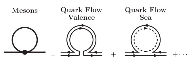
Figure 1: An example of a meson (thick line) loop diagram (left) with the quark diagrams (right), there are gluons all over in the right diagrams. The Valence (arrow line) and Sea (dash arrow line) quarks can be treated independently in lattice QCD.

A more extended discussion can be found in BG ; Sharpe . The version of ChPT with sea and valence quarks separately is called Partially Quenched ChPT (PQChPT).

3 Two Loop: General

The Lagrangians needed at the first three orders, $p^{2}$, $p^{4}$ and $p^{6}$, are known and the number of parameters and their notation are shown in Tab. 1.

	2 flavor		3 flavor		3+3 PQChPT
$p^{2}$	$F,B$	2	$F_{0},B_{0}$	2	$F_{0},B_{0}$	2
$p^{4}$	$l_{i}^{r},h_{i}^{r}$	7+3	$L_{i}^{r},H_{i}^{r}$	10+2	$\hat{L}_{i}^{r},\hat{H}_{i}^{r}$	11+2
$p^{6}$	$c_{i}^{r}$	53+4	$C_{i}^{r}$	90+4	$K_{i}^{r}$	112+3

Table 1: The number of free parameters and their names for the first three orders in mesonic ChPT. The numbers refer to the number of low energy constants and unmeasurable (high energy) constants.

The parameters at order $p^{2}$ go back very long time. The classification and infinities at $p^{4}$ can be found in GL1 ; GL2 and at $p^{6}$ in BCE1 ; BCE2 . The knowledge of the infinities provides a very useful check on explicit calculations.

The replica method allows to obtain PQChPT from the $n_{F}$ flavor case of BCE1 ; BCE2 . Important is that the 3 flavor case is a limit of the 3+3 PQChPT one. Determining the parameters in PQChPT allows to obtain those of 3 flavor ChPT via the Cayley-Hamilton relations of BCE1 .

4 Two Loop: 2 Flavours

In this case most calculations have already been performed.
$\bullet$ $\gamma\gamma\to\pi^{0}\pi^{0}$ BGS . $\bullet$ $\gamma\gamma\to\pi^{+}\pi^{-}$, $F_{\pi}$, $m_{\pi}$ Burgi . $\bullet$ $\pi\pi$-scattering, $F_{\pi}$, $m_{\pi}$ BCEGS . $\bullet$ $F_{V\pi}(t)$, $F_{S\pi}$ BCT . $\bullet$ $\pi\to\ell\nu\gamma$ BT1 . Here there is in general a rather good convergence and it turns out that for many threshold quantities the values of the $c^{i}_{r}$ are not numerically important. These calculations are now often combined with dispersive methods for very precise theoretical predictions. An example is the full description of $\pi\pi$ scattering CGL .

5 Two Loop: PQChPT

This subject is only beginning. The charged pion mass for the case of all valence masses equal and all 3 sea quark masses equal is published BDL and the result for the decay constant in this case will be published soon. Planned future work includes all the necessary mass combinations as well as the two sea quark case.

In the actual calculations heavy use is made of the symbolic manipulation program FORM FORM . The major problem is simply the sheer size of the expressions involved in the more general mass case due to the appearance in PQChPT of many partial fractions of differences of quark masses. An example of results is shown in Fig. 2.

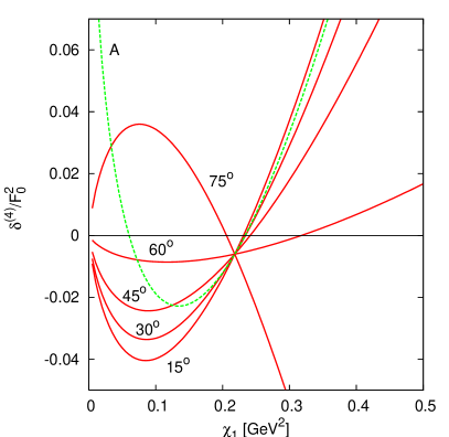
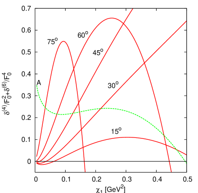
Figure 2: First results from PQChPT at two-loop level BDL . Shown is the relative correction to the lowest order mass squared at order $p^{4}$ (left) and $p^{4}+p^{6}$ (right). The valence quark mass is given as $\chi_{1}=2B_{0}m_{qV}$ and the sea quark mass as $\chi_{4}=2B_{0}m_{qS}$ with $\chi_{4}=\chi_{1}\,\tan\theta$ (curves labeled with angle $\theta$) or $\chi_{4}=0.125$ GeV² (A). $\chi_{i}$ corresponds to the lowest order meson mass squared. The boundary for ChPT is reached for some mass squared around 0.3 GeV²

6 Two Loop: 3 Flavor Overview and $\pi\pi$, $\pi K$ scattering

Many calculations have been performed here. A (to my knowledge) complete list is given below, where the quantities which are determined from this calculation are shown in brackets. The symbol $\Pi_{IJM}$ means a two-point Green function of currents $I$ and $J$ with the quantum numbers of meson $M$.
$\bullet$ $\Pi_{VV\pi}$, $\Pi_{VV\eta}$ GK1 ; ABT1 $\bullet$ $\Pi_{VVK}$ ABT1 ; DK $\bullet$ $\Pi_{AA\pi}$, $\Pi_{AA\eta}$, $F_{\pi,\eta}$, $m_{\pi,\eta}$, ABT1 ; GK2 $\bullet$ $\Pi_{SS}$ Moussallam ($L_{4}^{r},L_{6}^{r}$) $\bullet$ $\Pi_{VVK}$, $\Pi_{AAK}$, $F_{K}$, $m_{K}$ ABT1 $\bullet$ $K_{\ell 4}$ ABT2 ($L_{1}^{r},L_{2}^{r},L_{3}^{r}$) $\bullet$ $F_{\pi,K,\eta}$, $m_{\pi,K,\eta}$ $(m_{u}\neq m_{d})$ ABT3 ($L_{5,7,8}^{r},m_{u}/m_{d}$) $\bullet$ $F_{V\pi}$, $F_{VK^{+}}$, $F_{VK^{0}}$ PS ; BT2 ($L_{9}^{r}$) $\bullet$ $K_{\ell 3}$ PS ; BT3 ($V_{us}$) $\bullet$ $F_{S\pi}$, $F_{SK}$ BD ($L_{4}^{r},L_{6}^{r}$) $\bullet$ $K,\pi\to\ell\nu\gamma$ GHW ($L_{10}^{r}$) $\bullet$ $\pi\pi$ BDT1 $\bullet$ $\pi K$ BDT2
We now perform a general fit to experiment and check how well the whole system works and determine as many parameters as possible. First we need to identify a series of basic inputs to determine most of the parameters. The procedure is described in detail in ABT2 ; ABT3 . The actual inputs used are

• $K_{\ell 4}$: $F(0)$, $G(0)$, $\lambda$ from the E865 BNL experiment Pislak .

• $m^{2}_{\pi^{0}}$, $m^{2}_{\eta}$, $m_{K^{+}}^{2}$, $m_{K^{0}}^{2}$ Electromagnetic corrections including quark mass effectsDashen .

• $F_{\pi^{+}}=92.4$ MeV, $F_{K^{+}}/F_{\pi^{+}}=1.22\pm 0.01$, $2m_{s}/(m_{u}+m_{d})=24$ or $26$.

• $L_{4}^{r},L_{6}^{r}$.

• The $C_{i}^{r}$ as estimated using single resonance approximation.

These fits are performed varying the resonance input used for the $C_{i}^{r}$ by varying the size by an overall factor of two and the scale at which the saturation is applied. The final fitting result with errors is shown for some typical inputs in Tab. 2. The $C_{i}^{r}$ can be determined from experiment in several cases. When the dependence is purely kinematical, e.g. curvature of a form-factor, it works reasonably well BCT ; BT2 . For those with a mixed quark mass-kinematical dependence, e.g. the slope of $f_{+}(t)$ in $K_{\ell 3}$ it works OK BT3 . The remaining ones are difficult to estimate, the question here is what type of scalar to use, we know it is not the sigma BCT ; BD but what else is an open question.

The whole procedure is repeated for a range of input values of $L_{4}^{4},L_{6}^{r}$. Some examples of the fits are given in Tab. 2 where we quote the main fit (labeled fit 10), the same one but at $p^{4}$ order rather than $p^{6}$ as well as two with $L_{4}^{4},L_{6}^{r}\neq 0$. Fit B is one where all scalar form factors behave nicely BD while fit D is the one where the threshold parameters for $\pi\pi$ and $\pi K$ scattering are well fitted as discussed in more detail in BDT2 . Fig. 3 shows the constraints from $\pi\pi$ and $\pi K$ scattering as well as the region of fit D.

	fit 10	same $p^{4}$	fit B	fit D
$10^{3}L_{1}^{r}$	$0.43\pm 0.12$	$0.38$	$0.44$	$0.44$
$10^{3}L_{2}^{r}$	$0.73\pm 0.12$	$1.59$	$0.60$	$0.69$
$10^{3}L_{3}^{r}$	$-2.53\pm 0.37$	$-2.91$	$-2.31$	$-2.33$
$10^{3}L_{4}^{r}$	$\equiv 0$	$\equiv 0$	$\equiv 0.5$	$\equiv 0.2$
$10^{3}L_{5}^{r}$	$0.97\pm 0.11$	$1.46$	$0.82$	$0.88$
$10^{3}L_{6}^{r}$	$\equiv 0$	$\equiv 0$	$\equiv 0.1$	$\equiv 0$
$10^{3}L_{7}^{r}$	$-0.31\pm 0.14$	$-0.49$	$-0.26$	$-0.28$
$10^{3}L_{8}^{r}$	$0.60\pm 0.18$	$1.00$	$0.50$	$0.54$
$2B_{0}\hat{m}/m_{\pi}^{2}$	0.736	0.991	1.129	0.958
$m_{\pi}^{2}$: $p^{4},p^{6}$	0.006,0.258	0.009,$\equiv 0$	$-$0.138,0.009	$-$0.091,0.133
$m_{K}^{2}$: $p^{4},p^{6}$	0.007,0.306	0.075,$\equiv 0$	$-$0.149,0.094	$-$0.096,0.201
$m_{\eta}^{2}$: $p^{4},p^{6}$	$-$0.052,0.318	0.013,$\equiv 0$	$-$0.197,0.073	$-$0.151,0.197
$m_{u}/m_{d}$	0.45$\pm$0.05	0.52	0.52	0.50
$F_{0}$ [MeV]	87.7	81.1	70.4	80.4
$\frac{F_{K}}{F_{\pi}}$: $p^{4},p^{6}$	0.169,0.051	0.22,$\equiv 0$	0.153,0.067	0.159,0.061

Table 2: The results of the fits for several input values of $L_{4}^{r},L_{6}^{r}$, see text.

7 Two Loop: $K_{\ell 3}$ and $V_{us}$

The CKM matrix element $V_{us}$ is a fundamental parameter we like to determine as precisely as possible. In addition, the relation $|V_{ud}|^{2}+|V_{us}|^{2}=1$ is broken at about the two sigma level by the experimental values quoted in the PDG 2002PDG2002 . It is thus important to update both theory and experiment. The theory LR has been updated in several ways. The photonic corrections have been properly calculated in the modern ChPT language Cirigliano and the form factors $f_{+}(t)$, $f_{-}(t)$ are known to $p^{6}$ in ChPT PS ; BT3 .

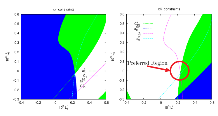
Figure 3: The constraints on $L_{4}^{r},L_{6}^{r}$ from $\pi\pi$ (left) and $\pi K$ (right) scattering BDT1 ; BDT2 .

The experiments have been mainly analyzed by assuming a linear parameterization of the form-factor. This is not sufficient as was pointed out in BT3 . The value of $|f_{+}(0)V_{us}|$ changes by 0.9% (0.6%), data from CPLEAR (PSE246 ), when a linear fit is used as compared with a quadratic one where the curvature is determined from ChPT BT3 . The newer experiments KTeV ; ISTRA have now detected the curvature and find values in agreement with the ChPT prediction of BT3 . The measured branching ratio in both the neutral and charged channel has also increased, KTeV ; BNL ; KLOE . Both combined lead to an increase in the value of $|f_{+}(0)V_{us}|$ and using the value of $f_{+}(0)$ from LR the unitarity problem is resolved.

The remaining problem is to accurately predict the value of $f_{+}(0)$. In LR one-loop ChPT and a quark model estimate of the higher orders were used. The $p^{6}$ calculation gives loop corrections of about one % to the one loop result PS ; BT3 . The full analysis including updated values of all the inputs is in BT3 but a more important point was made in BT3 as well. The $p^{6}$ low energy constants that appear in the value of $f_{+}(0)$ can be determined experimentally from the scalar form factor $f_{0}(t)$ since BT3

$$f_{0}(t) = 1-\frac{8}{F_{\pi}^{4}}{\left(C_{12}^{r}+C_{34}^{r}\right)}\left(m_{K}^{2}-m_{\pi}^{2}\right)^{2}+8\frac{t}{F_{\pi}^{4}}{\left(2C_{12}^{r}+C_{34}^{r}\right)}\left(m_{K}^{2}+m_{\pi}^{2}\right)$$ (2)

$$+\frac{t}{m_{K}^{2}-m_{\pi}^{2}}\left(F_{K}/F_{\pi}-1\right)-\frac{8}{F_{\pi}^{4}}t^{2}{C_{12}^{r}}+\overline{\Delta}(t)+\Delta(0)\,.$$

In this equation everything is known except the values of $C_{12}^{r}$ and $C_{34}^{r}$, and correlations between $F_{K}/F_{\pi}$ and $V_{us}$knecht . Since $f_{+}(0)=f_{0}(0)$ a measurement of the slope and curvature of the scalar form factor allows to determine $f_{+}(0)$. Dispersion theory allows to relate some of these quantities as well. A first analysis JOP leads to an estimate that essentially cancels the pure loop contribution yielding a very small total $p^{6}$ correction.

8 Conclusions

The two flavor case in ChPT at two loops is an almost finished subject. The three flavor case is in progress. Many calculations have been done and things seem to work but convergence is sometimes slow. $L_{4}^{r},L_{6}^{r}$ are nonzero but reasonable for large $N_{c}$ expectations. An example of clean predictions even with the many $p^{6}$ constants is the case of $K_{\ell 3}$ decays and the determination of $V_{us}$. The partially quenched case, relevant for lattice calculations, is just at its beginnings at two loop order.

References

- (1) S. Weinberg, Physica A96, 327 (1979).
- (2) J. Gasser and H. Leutwyler, Annals Phys. 158, 142 (1984).
- (3) J. Gasser and H. Leutwyler, Nucl. Phys. B 250, 465 (1985).
- (4) S. Scherer, hep-ph/0210398; G. Ecker, hep-ph/0011026; A. Pich, hep-ph/9806303.
- (5) C. W. Bernard and M. F. L. Golterman, Phys. Rev. D 46, 853 (1992) [hep-lat/9204007].
- (6) S. R. Sharpe and N. Shoresh, Phys. Rev. D 62, 094503 (2000) [hep-lat/0006017].
- (7) J. Bijnens, G. Colangelo and G. Ecker, JHEP 9902, 020 (1999) [hep-ph/9902437].
- (8) J. Bijnens, G. Colangelo and G. Ecker, Annals Phys. 280, 100 (2000) [hep-ph/9907333].
- (9) S. Bellucci, J. Gasser and M. E. Sainio, Nucl. Phys. B 423, 80 (1994) [hep-ph/9401206].
- (10) U. Bürgi, Phys. Lett. B 377, 147 (1996) [hep-ph/9602421], Nucl. Phys. B 479, 392 (1996) [hep-ph/9602429].
- (11) J. Bijnens et al., Phys. Lett. B 374, 210 (1996) [hep-ph/9511397], Nucl. Phys. B 508, 263 (1997) [Erratum-ibid. B 517, 639 (1998)] [hep-ph/9707291].
- (12) J. Bijnens, G. Colangelo and P. Talavera, JHEP 9805, 014 (1998) [hep-ph/9805389].
- (13) J. Bijnens and P. Talavera, Nucl. Phys. B 489, 387 (1997) [hep-ph/9610269].
- (14) G. Colangelo, J. Gasser and H. Leutwyler, Nucl. Phys. B 603, 125 (2001) [hep-ph/0103088].
- (15) J. Bijnens, N. Danielsson and T. A. Lähde, hep-lat/0406017.
- (16) J. A. Vermaseren, math-ph/0010025.
- (17) E. Golowich and J. Kambor, Nucl. Phys. B 447, 373 (1995) [hep-ph/9501318].
- (18) G. Amorós, J. Bijnens and P. Talavera, Nucl. Phys. B 568, 319 (2000) [hep-ph/9907264].
- (19) S. Dürr and J. Kambor, Phys. Rev. D 61, 114025 (2000) [hep-ph/9907539].
- (20) E. Golowich and J. Kambor, Phys. Rev. D 58, 036004 (1998) [hep-ph/9710214].
- (21) B. Moussallam, JHEP 0008, 005 (2000) [hep-ph/0005245].
- (22) G. Amorós, J. Bijnens and P. Talavera, Phys. Lett. B 480, 71 (2000) [hep-ph/9912398], Nucl. Phys. B 585, 293 (2000) [Erratum-ibid. B 598, 665 (2001)] [hep-ph/0003258].
- (23) G. Amorós, J. Bijnens and P. Talavera, Nucl. Phys. B 602, 87 (2001) [hep-ph/0101127].
- (24) P. Post and K. Schilcher, Eur. Phys. J. C 25, 427 (2002) [hep-ph/0112352].
- (25) J. Bijnens and P. Talavera, JHEP 0203, 046 (2002) [hep-ph/0203049].
- (26) J. Bijnens and P. Talavera, Nucl. Phys. B 669, 341 (2003) [hep-ph/0303103].
- (27) J. Bijnens and P. Dhonte, JHEP 0310, 061 (2003) [hep-ph/0307044].
- (28) C. Q. Geng, I. L. Ho and T. H. Wu, Nucl. Phys. B 684, 281 (2004) [hep-ph/0306165].
- (29) J. Bijnens, P. Dhonte and P. Talavera, JHEP 0401, 050 (2004) [hep-ph/0401039].
- (30) J. Bijnens, P. Dhonte and P. Talavera, JHEP 0405, 036 (2004) [hep-ph/0404150].
- (31) S. Pislak et al., Phys. Rev. D 67, 072004 (2003) [hep-ex/0301040].
- (32) J. Bijnens and J. Prades, Nucl. Phys. B 490, 239 (1997) [hep-ph/9610360].
- (33) K. Hagiwara et al. [Particle Data Group Collaboration], Phys. Rev. D 66 (2002) 010001.
- (34) H. Leutwyler and M. Roos, Z. Phys. C 25, 91 (1984).
- (35) V. Cirigliano et al., Eur. Phys. J. C 23, 121 (2002) [hep-ph/0110153].
- (36) A. Apostolakis et al. [CPLEAR Collaboration], Phys. Lett. B 473, 186 (2000).
- (37) A. S. Levchenko et al. [KEK-PS E246 Collaboration], Yad. Fiz. 65, 2294 (2002) [hep-ex/0111048].
- (38) T. Alexopoulos et al. [KTeV Collaboration], hep-ex/0406001, hep-ex/0406003.
- (39) O. P. Yushchenko et al., Phys. Lett. B 589, 111 (2004) [hep-ex/0404030].
- (40) A. Sher et al., Phys. Rev. Lett. 91, 261802 (2003) [hep-ex/0305042].
- (41) P. Franzini, hep-ex/0408150.
- (42) N. H. Fuchs, M. Knecht and J. Stern, Phys. Rev. D 62, 033003 (2000) [hep-ph/0001188].
- (43) M. Jamin, J. A. Oller and A. Pich, JHEP 0402, 047 (2004) [hep-ph/0401080].