Probing the gauge bosons $Z^{\prime}$ and $B^{\prime}$ from the littlest Higgs model in the high-energy linear $e^{+}e^{-}$ colliders

Abstract

The littlest Higgs (LH) model predicts the existence of the new gauge bosons $Z^{\prime}$ and $B^{\prime}$. We calculate the contributions of these new particles to the processes $e^{+}e^{-}\rightarrow\overline{f}f$ with $f=\tau,\mu,b,$ or $c$ and study the possibility of detecting these new particles via these processes in the future high-energy linear $e^{+}e^{-}$ collider (LC) experiments with $\sqrt{s}=500GeV$ and $\pounds_{int}=340fb^{-1}$. We find that, with reasonable values of the parameter preferred by the electroweak precision data, the possible signals of these new particles might be detected. The $Z^{\prime}$ mass $M_{Z^{\prime}}$ can be explored up to $2.8TeV$ via the process $e^{+}e^{-}\rightarrow\overline{b}b\$ for $0.3\leq c\leq 0.5$ and the $B^{\prime}$ mass $M_{B^{\prime}}$ can be explored up to $1.26TeV$ via the process $e^{+}e^{-}\rightarrow\overline{l}l\$ for $0.64\leq c^{\prime}\leq 0.73$.

PACS number: 12.60.Cn, 13.66De, 14.70.Pw

I. Introduction

The hadron colliders, such as the Tevatron and the future LHC, are expected to directly probe possible new physics beyond the standard model(SM) up to a scale of a few $TeV$, while a high-energy linear $e^{+}e^{-}$ collider (LC) is required to complement the probe of the new particles with detailed measurement[1]. Some kinds of new physics predict the existence of new particles that will be manifested as a rather spectacular resonance in the LC experiments if the achievable center-of-mass(c.m.) energy $\sqrt{s}$ is sufficient. Even if their masses exceed the c.m. energy $\sqrt{s}$, the LC experiments also retain an indirect sensitivity through a precision study of their virtual corrections to electroweak observables. Thus, a future LC, such as the Giga $Z$ option of the LC, will offer an excellent opportunity to study new physics with uniquely high precision.

Little Higgs models[2, 3, 4] were recently proposed as a kind of models of electroweak symmetry breaking(EWSB), which can be regarded as one of the important candidates of the new physics beyond the SM. Little Higgs models employ an extended set of global gauge symmetries in order to avoid the one-loop quadratic divergences and thus provide a new approach to solve the hierarchy between the $TeV$ scale of possible new physics and the electroweak scale, $v=246GeV=(\sqrt{2}G_{F})^{-\frac{1}{2}}$. In these models, at least two interactions are needed to explicitly break all of the global symmetries, which forbid quadratic divergences in Higgs mass at one-loop level. EWSB is triggered by the Colemean-Weinberg Potential, which is generated by integrating out the heavy degrees of freedom. In this kind of models, the Higgs boson is a pseudo-Goldstone boson of a global symmetry which is spontaneously broken at some high scale $f$ by an vacuum expectation value($vev$) and thus is naturally light. A general feature of this kind of models is that the cancellation of the quadratic divergences is realized between particles of the same statistics.

Little Higgs models are weakly interaction models, which contain extra gauge bosons, new scalars and fermions, apart from the SM particles. These new particles might produce characteristic signatures at the present and future collider experiments[5, 6, 7, 8, 9, 10]. Since the extra gauge bosons can mix with the SM gauge bosons $W$ and $Z$, the masses of the SM gauge bosons $W$ and $Z$ and their couplings to the SM particles are modified from those in the SM at the order of $v^{2}/f^{2}$. Thus, the precision measurement data can give severe constraints on this kind of models[5, 11, 12, 13, 14, 15, 16, 17].

In general, the new gauge bosons are heavier than the current experimental limits on direct searches. However, these new particles may have effects at low energy by contributing to higher dimension operators in the SM after integrating them out, which might generate observable signals in the present or future experiments. For example, Ref.[17] has shown that $Z^{{}^{\prime}}$ exchange and $B^{{}^{\prime}}$ exchange can give correction effects on the four-fermion interactions in the context of the little Higgs models. In this paper, we will discuss the possibility of detecting the new neutral gauge bosons $Z^{{}^{\prime}}$ and $B^{{}^{\prime}}$ in the future LC experiments with the c.m. energy $\sqrt{s}=500GeV$ and the integrating luminosity $\pounds_{int}=340fb^{-1}$ and both beams polarized[1] via considering their contributions to the processes $e^{+}e^{-}\rightarrow\overline{f}f$ with $f=\tau,\mu,b$ and $c$ in the context of the littlest Higgs(LH) model[2]. We find that these new gauge bosons can indeed produce significant contributions to these processes in wide range of the parameter space [$0\leq c\leq 0.5,0.62\leq c^{\prime}\leq 0.73$] preferred by the electroweak precision data. The new gauge bosons $Z^{{}^{\prime}}$ and $B^{{}^{\prime}}$ might be observable in the future LC experiments.

The LH model has all essential features of the little Higgs models. So, in the rest of this paper, we give our results in detail in the framework of the LH model, although many alternatives have been proposed[3, 4]. Section II contains a short summary of the masses and the relevant couplings of the new gauge bosons $Z^{{}^{\prime}}$ and $B^{{}^{\prime}}$ to ordinary particles. The total decay widths of these new gauge bosons are also estimated. Section III is devoted to the calculation and analysis the relative corrections of the new gauge bosons $Z^{{}^{\prime}}$ and $B^{{}^{\prime}}$ to the cross sections of the processes $e^{+}e^{-}\rightarrow\overline{f}f$ with $f=\tau,\ \mu,\ b$ and $c$. In Section IV, we proceed to a comparison of the discovery potential of each process in the future LC experiment with $\sqrt{s}=500GeV$ and $\pounds_{int}=340fb^{-1}$. Our conclusions and discussions are given in Section V.

II. The masses and the relevant couplings of the gauge bosons $Z^{{}^{\prime}}$ and $B^{{}^{\prime}}$

As the simplest realization of the little Higgs idea, the LH model $[2]$ consists of a non-linear $\sigma$ model with a global $SU(5)$ symmetry which is broken down to $SO(5)$ by a vacuum condensate $f$ $\sim\Lambda_{s}/4\pi\sim TeV$, which results in fourteen massless Goldstone bosons. Four of these massless Goldstone bosons are eaten by the SM gauge bosons, so that the locally gauged symmetry $SU(2)_{1}\times U(1)_{1}\times SU(2)_{2}\times U(1)_{2}$ is broken down to its diagonal subgroup $SU(2)\times U(1)$, identified as the $SM$ electroweak gauge group. The remaining ten Goldstone bosons transform under the $SM$ gauge group as a doublet H and a triplet $\Phi$. This breaking scenario also gives rise to the new gauge bosons, such as $Z^{{}^{\prime}}$ and $B^{{}^{\prime}}$. The masses of the neutral gauge bosons $Z^{{}^{\prime}}$ and $B^{{}^{\prime}}$ can be written at the order of $v^{2}/f^{2}$[5]:

$$M_{Z^{\prime}}^{2} = M_{Z}^{2}C_{W}^{2}[\frac{f^{2}}{s^{2}c^{2}v^{2}}-1-\frac{5S_{W}^{3}}{2C_{W}}\frac{sc(c^{2}s^{\prime 2}+s^{2}c^{\prime 2})}{s^{\prime}c^{\prime}(5C_{W}^{2}s^{\prime 2}c^{\prime 2}-S_{W}^{2}s^{2}c^{2})}],$$ (1)

$$M_{B^{\prime}}^{2} = M_{Z}^{2}S_{W}^{2}[\frac{f^{2}}{5s^{\prime 2}c^{\prime 2}v^{2}}-1+\frac{5C_{W}^{3}}{8S_{W}}\frac{s^{\prime}c^{\prime}(c^{2}s^{\prime 2}+s^{2}c^{\prime 2})}{sc(5C_{W}^{2}s^{\prime 2}c^{\prime 2}-S_{W}^{2}s^{2}c^{2})}],$$ (2)

where $M_{Z}$ is the $Z$ mass predicted by the SM and $f$ is the scale parameter. Using the mixing parameters $c(s=\sqrt{1-c^{2}})$ and $c^{\prime}(s^{\prime}=\sqrt{1-c^{\prime 2}})$, we can represent the SM gauge coupling constants as $g=g_{1}s=g_{2}c$ and $g^{\prime}=g^{\prime}_{1}s^{\prime}=g^{\prime}_{2}c^{\prime}$. $S_{W}=\sin\theta_{W}$, $\theta_{W}$ is the Weinberg angle. From Eq.(1) and Eq.(2) we can see that the values of $M_{Z^{\prime}}$ and $M_{B^{\prime}}$ are mainly dependent on the value of the scale parameters $(f,c)$, and $(f,c^{\prime})$, respectively. In general, the gauge boson $B^{\prime}$ is substantially lighter than the gauge boson $Z^{\prime}$. Considering the constraints of the electroweak precision data on the free parameters $f,\ c,$ and $c^{\prime}$ in the LH model, the value of the ratio $M_{B^{\prime}}^{2}/M_{Z^{\prime}}^{2}$ can be further reduced[8].

In the LH model, the couplings of the neutral gauge bosons $Z$, $Z^{{}^{\prime}}$ and $B^{{}^{\prime}}$ to fermions can be written as:

$$e[(g_{L}^{f}+\delta g_{L}^{f})\overline{f_{L}}\gamma^{\mu}f_{L}+(g_{R}^{f}+\delta g_{R}^{f})\overline{f_{R}}\gamma^{\mu}f_{R}]Z_{\mu}$$

$$+e[g_{L}^{Zf}\overline{f_{L}}\gamma^{\mu}f_{L}+g_{R}^{Zf}\overline{f_{R}}\gamma^{\mu}f_{R}]Z^{\prime}_{\mu}+e[g_{L}^{Bf}\overline{f_{L}}\gamma^{\mu}f_{L}+g_{R}^{Bf}\overline{f_{R}}\gamma^{\mu}f_{R}]B^{\prime}_{\mu}$$ (3)

with

$$g_{L}^{f}=\frac{1}{S_{W}C_{W}}(I_{3}^{f}-Q_{f}S_{W}^{2}),\hskip 14.22636ptg_{R}^{f}=\frac{1}{S_{W}C_{W}}(-Q_{f}S_{W}^{2}).$$ (4)

Where $I_{3}^{f}$ is the third component of fermion isospin and $Q_{f}$ is the electric charge of fermion $f$ in units of the position charge $e$. The $\delta g_{L}^{f}$ and $\delta g_{R}^{f}$ represent the correction terms of the tree-level $Z\overline{f}f$ couplings $g_{L}^{f}$ and  $g_{R}^{f}$, which come from the mixing between the gauge boson $Z^{\prime}$ and the SM gauge boson $Z$. The general forms of these terms have been given in Ref.[5]. The relevant forms, which are related the processes $e^{+}e^{-}\rightarrow$ $\overline{f}f$($f=l$, $b$ and $c$) can be written as:

$$g_{R}^{Zf} = 0,\hskip 28.45274ptg_{L}^{Zu}=-g_{L}^{Zd}=-g_{L}^{Zl}=\frac{1}{S_{W}}\frac{c}{2s},$$ (5)

$$g_{L}^{Bl} = \frac{1}{C_{W}}\frac{1}{2s^{\prime}c^{\prime}}(c^{\prime 2}-\frac{2}{5}),\hskip 28.45274ptg_{R}^{Bl}=\frac{1}{C_{W}}\frac{1}{s^{\prime}c^{\prime}}(c^{\prime 2}-\frac{2}{5}),$$ (6)

$$g_{L}^{Bb} = -\frac{1}{C_{W}}\frac{1}{6s^{\prime}c^{\prime}}(c^{\prime 2}-\frac{2}{5}),\hskip 28.45274ptg_{R}^{Bb}=\frac{1}{C_{W}}\frac{1}{3s^{\prime}c^{\prime}}(c^{\prime 2}-\frac{2}{5}),$$ (7)

$$g_{L}^{Bc} = -\frac{1}{C_{W}}\frac{1}{6s^{\prime}c^{\prime}}(c^{\prime 2}-\frac{2}{5}),\hskip 28.45274ptg_{R}^{Bc}=-\frac{1}{C_{W}}\frac{2}{3s^{\prime}c^{\prime}}(c^{\prime 2}-\frac{2}{5}),$$ (8)

where $l=\tau,\mu$ or $e$. The couplings of the gauge boson $B^{\prime}$ to fermions are quite model dependent, which depend on the choice of the fermion $U(1)$ charges under the two $U(1)$ groups[5, 13]. The $U(1)$ charges of the SM fermions are constrained by requiring that the Yukawa couplings are gauge invariant and maintaining the usual SM hypercharge assignment. Combing the gauge invariance of the Yukawa couplings with the $U(1)$ anomaly-free can fix all of the $U(1)$ charge values. The couplings of the $B^{\prime}$ with fermions given by Eqs.(6)–(8) come from this kind of choice. Certainly, this is only one example of all possible $U(1)$ charge assignments. In other little Higgs models, several alternatives for the $U(1)$ charge choice exist[3, 4, 13].

In the LH model, the custodial $SU(2)$ global symmetry is explicitly broken, which can generate large contributions to the electroweak observables. If one assumes that the SM fermions are charged only under $U(1)_{1}$, then global fits to the electroweak precision data produce rather severe constraints on the parameter space of the LH model[11, 12]. However, if the SM fermions are charged under $U(1)_{1}\times U(1)_{2}$, the constraints become relaxed. The scale parameter $f=1\sim 2TeV$ is allowed for the mixing parameters $c$ and $c^{\prime}$ in the ranges of $0\sim 0.5$ and $0.62\sim 0.73$, respectively[13, 14]. On the other hand, the neutral gauge boson $B^{\prime}$ is typically light and should produce significantly contributions to observables. Thus, it can be seen as the first signal of the LH model. The production and the possible signals of the $B^{\prime}$ at the hadron colliders(Tevatron or LHC) have been studied in Refs[5, 11, 14]. It has been shown that the gauge boson $B^{\prime}$ is excluded for a mass lower than $500GeV$ by the direct search at the Tevatron. However, Ref.[8] has shown that a large portion of the parameter space consistent with the electroweak precision data can accommodate the Tevatron direct searches to new gauge bosons decaying into dileptons. The light $B^{\prime}$ is not excluded by the direct searches for the neutral gauge boson at the Tevatron. So, we will take the $M_{Z^{\prime}}$, $M_{B^{\prime}}$ and the mixing parameters $c,c^{\prime}$ as free parameters in our discussions, which are assumed in the ranges of $1TeV\sim 3TeV$, $400GeV\sim 1000GeV$, $0.1\sim 0.5$ and $0.62\sim 0.73$, respectively.

Figure 1: The total decay width $\Gamma_{Z^{\prime}}$ as a function of the $Z^{\prime}$ mass $M_{Z^{\prime}}$ for $c=0.1$(solid                 line), $c=0.3$(dashed line) and $c=0.5$(dotted line).

At the leading order, the two-body decay channels of the neutral gauge boson $V(Z^{\prime}$ or $B^{\prime})$ mainly contain $V\rightarrow\overline{f}f$, where $f$ is any of the SM quarks or leptons, and $V\rightarrow Zh$. If we ignore the fermion masses, the generic partial decay width for $V$ to fermion pair can be written as [5, 7]:

$$\Gamma(V\rightarrow\overline{f}f)=\frac{C}{24\pi}[(g_{L}^{Vff})^{2}+(g_{R}^{Vff})^{2}]M_{V},$$ (9)

where $C$ is the fermion color factor and $C=1$(3) for leptons(quarks). For the gauge boson $Z^{\prime}$, the total decay width can be approximately written as:

$$\Gamma_{Z^{\prime}} = 6\Gamma(Z^{\prime}\rightarrow\overline{q}q)+6\Gamma(Z^{\prime}\rightarrow\overline{l}l)+\Gamma(Z^{\prime}\rightarrow Zh)+\Gamma(Z^{\prime}\rightarrow W^{+}W^{-})$$ (10)

$$\approx \frac{\alpha_{e}M_{Z^{\prime}}}{96S_{W}^{2}}[\frac{96c^{2}}{s^{2}}+\frac{(c^{2}-s^{2})^{2}}{s^{2}c^{2}}].$$

In general, the $B^{\prime}$ mass $M_{B^{\prime}}$ is not too large and can be allowed to be in the range of a few hundred $GeV$. So, for the decay channels $B^{\prime}\rightarrow\overline{t}t$ and $B^{\prime}\rightarrow Zh$, we can not neglect the final state masses. The total decay width of the gauge boson $B^{\prime}$ can be written as:

$$\Gamma_{B^{\prime}} = 3\Gamma(B^{\prime}\rightarrow\overline{l}l)+3\Gamma(B^{\prime}\rightarrow\overline{\nu}\nu)+3\Gamma(B^{\prime}\rightarrow\overline{d}d)$$ (11)

$$+2\Gamma(B^{\prime}\rightarrow\overline{u}u)+\Gamma(B^{\prime}\rightarrow\overline{t}t)+\Gamma(B^{\prime}\rightarrow Zh)$$

$$\approx \frac{\alpha_{e}M_{B^{\prime}}}{4C_{W}^{2}}\{{\frac{85(c^{\prime 2}-\frac{2}{5})^{2}}{18s^{\prime 2}c^{\prime 2}}+\frac{\sqrt{1-4r_{t}}}{s^{\prime 2}c^{\prime 2}}\{[\frac{5}{6}(\frac{2}{5}-c^{\prime 2})-\frac{1}{5}x_{L}]^{2}}(1+2r_{t})$$

$$+[\frac{1}{2}(\frac{2}{5}-c^{\prime 2})-\frac{1}{5}x_{L}]^{2}(1-4r_{t})\}+\frac{(c^{\prime 2}-s^{\prime 2})^{2}}{24c^{\prime 2}s^{\prime 2}}\lambda^{\frac{1}{2}}[(1+r_{Z}-r_{h})^{2}+8r_{Z}]\},$$

where $r_{i}=m_{i}^{2}/M_{B^{\prime}}^{2}$ and $\lambda=1+r_{Z}^{2}+r_{h}^{2}+2r_{Z}+2r_{h}+2r_{Z}r_{h}$. The mixing parameter between the SM top quark $t$ and the vector-like quark $T$ is defined as $x_{L}=\lambda_{1}^{2}/(\lambda_{1}^{2}+\lambda_{2}^{2})$, in which $\lambda_{1}$ and $\lambda_{2}$ are the coupling parameters. In above equation, we have neglected the decay width $\Gamma(B^{\prime}\rightarrow W^{+}W^{-})$, which is suppressed by a factor of $\nu^{4}/f^{4}$.

From above equations, we can see that the total decay width $\Gamma_{Z^{\prime}}$ is mainly dependent on the free parameters $M_{Z^{\prime}}$ and $c$, while the total decay width $\Gamma_{B^{\prime}}$ is sensitive to the free parameters $M_{B^{\prime}}$ and $c^{\prime}$. For $c^{\prime}=\sqrt{2/5}$, the gauge boson $B^{\prime}$ mainly decays to $Zh$ and $t\overline{t}$, and the decay modes $l\overline{l}$ and $q\overline{q}(q\neq t)$ are prohibited being its couplings with the light fermions vanish. In Fig.1 and Fig.2, we plot $\Gamma_{Z^{\prime}}$ and $\Gamma_{B^{\prime}}$ as functions of $M_{Z^{\prime}}$ and $M_{B^{\prime}}$ for three values of $c$ and $c^{\prime}$, respectively. In Fig.2 we have taken $\lambda_{1}\approx\lambda_{2}$. From these figures, we can see that $\Gamma_{Z^{\prime}}$ is in tens and up to hundred $GeV$, while $\Gamma_{B^{\prime}}<1GeV$ in the parameter space preferred by the electroweak precision data.

In the following sections, we will use the above formulae to calculate the corrections of the neutral gauge bosons $Z^{\prime}$ and $B^{\prime}$ to the cross sections of the processes $e^{+}e^{-}\rightarrow\overline{f}f$ in the parameter space[ $0\leq c\leq 0.5$ and $0.62\leq c^{\prime}\leq 0.73$], which is consistent with the precision electroweak constraints. Then we will study the realistic observability of the gauge bosons $Z^{\prime}$ and $B^{\prime}$ in the future LC experiments.

Figure 2: The total decay width $\Gamma_{B^{\prime}}$ as a function of the $B^{\prime}$ mass $M_{B^{\prime}}$ for $c^{\prime}=0.65$(solid                 line), $c^{\prime}=0.68$(dashed line) and $c^{\prime}=0.71$(dotted line).

III. The contributions of $Z^{\prime}$ and $B^{\prime}$ to the processes $e^{+}e^{-}\rightarrow\overline{f}f$

Neglecting fermion mass $m_{f}$($f=\tau,\ \mu,\ b$ or $c$) with respect to the c.m. energy $\sqrt{s}$, the helicity cross sections $\sigma_{\alpha\beta}(\overline{f}f)$ of the processes $e^{+}e^{-}\rightarrow\overline{f}f$ can be given in Born approximation [18, 19]:

$$\sigma_{\alpha\beta}(\overline{f}f)=N_{c}A|M_{\alpha\beta}(\overline{f}f)|^{2},$$ (12)

where $\alpha$, $\beta=L,\ R$; $N_{c}=3(1+\frac{\alpha_{s}}{\pi})$ for quarks and $N_{c}=1$ for leptons. $A=\sigma(e^{+}e^{-}\rightarrow r^{*}\rightarrow\overline{f}f)=(4\pi\alpha_{e}^{2})/(3s)$. In the LH model, the helicity amplitude $M_{\alpha\beta}(\overline{f}f)$ can be written as:

$$M_{\alpha\beta}(\overline{f}f)=Q_{e}Q_{f}+(g_{\alpha}^{e}+\delta g_{\alpha}^{e})(g_{\beta}^{f}+\delta g_{\beta}^{f})\chi_{Z}+g_{\alpha}^{Ze}g_{\beta}^{Zf}\chi_{Z^{\prime}}+g_{\alpha}^{Be}g_{\beta}^{Bf}\chi_{B^{\prime}}$$ (13)

with

$$\chi_{i}=\frac{s}{s-M_{i}^{2}+iM_{i}\Gamma_{i}},$$ (14)

where $\chi_{i}$ represent the propagators of the gauge bosons $Z,\ Z^{\prime}$, and $B^{\prime}$, in which $\Gamma_{i}$ represents the corresponding total decay width. From above equation, we can see that the contributions of the LH model to the processes $e^{+}e^{-}\rightarrow\overline{f}f$ mainly come from three sources: (1) the modification to the relation between the SM free parameters, (2) the correction terms to the tree-level $Z\overline{f}f$ couplings, (3) $Z^{\prime}$ exchange and $B^{\prime}$ exchange.

The contributions of the neutral gauge bosons $Z^{\prime}$ and $B^{\prime}$ to the helicity cross sections $\sigma_{\alpha\beta}(\overline{f}f)$ can be written as:

$$\Delta\sigma_{\alpha\beta}(\overline{f}f) = \sigma_{\alpha\beta}^{ZB}(\overline{f}f)-\sigma_{\alpha\beta}^{SM}(\overline{f}f)$$ (15)

$$\approx 2N_{c}A[M_{\alpha\beta}^{SM}(\overline{f}f)g_{\alpha}^{Ze}g_{\beta}^{Zf}\chi_{Z^{\prime}}+M_{\alpha\beta}^{SM}(\overline{f}f)g_{\alpha}^{Be}g_{\beta}^{Bf}\chi_{B^{\prime}}].$$

In above equation, we have neglected the terms which are proportional to $(g_{\alpha}^{Bf})^{2}$ and $(g_{\alpha}^{Zf})^{2}$. This is because the contributions of these terms to the helicity cross sections are suppressed by the factor $\nu^{4}/f^{4}$. The first and second terms of the right-side of this equation represent the contributions of $Z^{\prime}$ exchange and $B^{\prime}$ exchange, respectively.

The cross sections $\sigma(\overline{f}f)$, which can be directly detected at the LC experiments, can be written as:

$$\sigma(\overline{f}f)=\frac{1}{4}[\sigma_{LL}(\overline{f}f)+\sigma_{LR}(\overline{f}f)+\sigma_{RL}(\overline{f}f)+\sigma_{RR}(\overline{f}f)].$$ (16)

To discuss the contributions of $Z^{\prime}$ exchange and $B^{\prime}$ exchange to the processes $e^{+}e^{-}\rightarrow\overline{f}f$, we define the relative correction parameters:

$$R_{1}(\overline{f}f)=\frac{\Delta\sigma_{1}(\overline{f}f)}{\sigma^{SM}(\overline{f}f)},\hskip 28.45274ptR_{2}(\overline{f}f)=\frac{\Delta\sigma_{2}(\overline{f}f)}{\sigma^{SM}(\overline{f}f)},$$ (17)

where $\Delta\sigma_{1}(\overline{f}f)$ and $\Delta\sigma_{2}(\overline{f}f)$ represent the contributions of $Z^{\prime}$ exchange and $B^{\prime}$ exchange, respectively. From above discussions, we can see that $R_{1}$ is mainly dependent on the free parameters $M_{Z^{\prime}}$ and $c$, $R_{2}$ is mainly dependent on the free parameters $M_{B^{\prime}}$ and $c^{\prime}$.

To see the contributions of the neutral gauge boson $Z^{\prime}$ to the processes $e^{+}e^{-}\rightarrow\overline{f}f$, we plot the relative correction parameters $R_{1}(\overline{l}l)(l=\mu$ or $\tau)$, $R_{1}(\overline{b}b)$, and $R_{1}(\overline{c}c)$ as functions of the $Z^{\prime}$ mass $M_{Z^{\prime}}$ for three values of the mixing parameter $c$ in Fig.3, Fig.4, and Fig.5, respectively. From these figures, we can see that $Z^{\prime}$ exchange generates negative contributions to all of these processes. The gauge boson $Z^{\prime}$ can decrease the production cross sections of the processes $e^{+}e^{-}\rightarrow\overline{f}f$. The contributions of $Z^{\prime}$ exchange to these processes increase as $M_{Z^{\prime}}$ decreasing and $c$ increasing. In all of the parameter space of the LH model, the contributions of $Z^{\prime}$ to the process $e^{+}e^{-}\rightarrow\overline{b}b$ are larger than those for the processes $e^{+}e^{-}\rightarrow\overline{l}l$ or $e^{+}e^{-}\rightarrow\overline{c}c$. For example, for $M_{Z^{\prime}}=1TeV$ and $c=0.5$, the absolute values of the relative correction parameter $R_{1}$ are $18.2\%$, $11.8\%$, $7.5\%$ for the processes $e^{+}e^{-}\rightarrow\overline{b}b$, $\overline{c}c$, and $\overline{l}l$, respectively. For $M_{Z^{\prime}}\geq 1.7TeV$ and $c\leq 0.5$, which satisfy the electroweak precision constraints[13,14], the absolute value of $R_{1}(\overline{f}f)$ are smaller than $5\%$, which is very difficult to be detected in the future LC experiments. However, if we assume $M_{Z^{\prime}}\leq 1.5TeV$ and $c>0.5$, the signal of the gauge boson $Z^{\prime}$ can be easy detected.

Figure 3: The relative correction parameter $R_{1}$ for the process $e^{+}e^{-}\rightarrow\overline{l}l$ as function                 of $M_{Z^{\prime}}$ for $c=0.1$(solid line), $c=0.3$(dashed line) and $c=0.5$(dotted line).

Figure 4: Same as Fig.3 but for the process $e^{+}e^{-}\rightarrow\overline{b}b$.

Figure 5: Same as Fig.3 but for the process $e^{+}e^{-}\rightarrow\overline{c}c$.

The relative correction parameters $R_{2}(\overline{f}f)$ with $f=l,\ b,\ c$ are plotted as functions of the $B^{\prime}$ mass $M_{B^{\prime}}$ for three values of the mixing parameter $c^{\prime}$ in Fig.6–8. Comparing these figures with Fig.3–5, we find that the contributions of gauge boson $B^{\prime}$ exchange to these processes are larger than those of gauge boson $Z^{\prime}$ exchange in wide range of the parameter space. This is mainly because the heavy photon $B^{\prime}$ is lighter than the gauge boson $Z^{\prime}$ in most of the parameter space of the LH model. However, the corrections of $B^{\prime}$ exchange to these processes may be positive or negative, which are dependent on the value of the $B^{\prime}$ mass $M_{B^{\prime}}$. The peak of the relative correction resonance emerges when the $B^{\prime}$ mass $M_{B^{\prime}}$ is approximately equal to $480GeV$ or $520GeV$ for the c. m. energy $\sqrt{s}=500GeV$.

Figure 6: The relative correction parameter $R_{2}$ for the process $e^{+}e^{-}\rightarrow\overline{l}l$ as function                 of $M_{B^{\prime}}$ for $c^{\prime}=0.65$(solid line), $c^{\prime}=0.68$(dashed line) and $c^{\prime}=0.71$(dotted                 line).

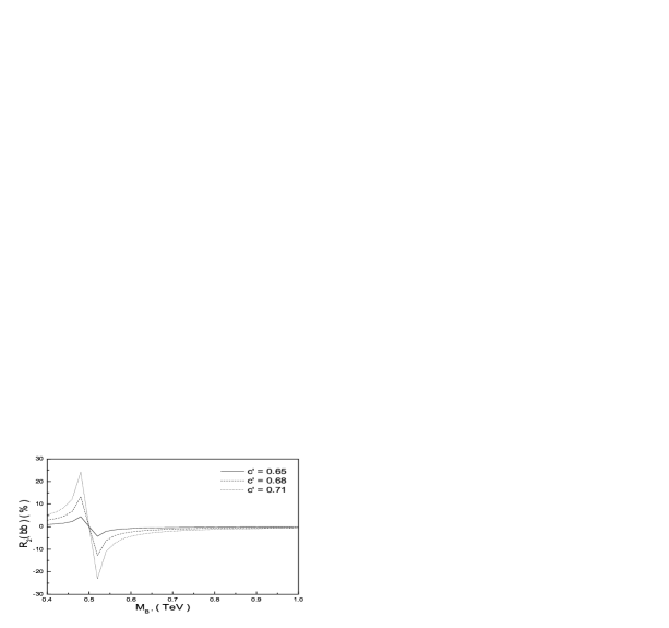
Figure 7: Same as Fig.6 but for the process $e^{+}e^{-}\rightarrow\overline{b}b$.

Figure 8: Same as Fig.6 but for the process $e^{+}e^{-}\rightarrow\overline{c}c$.

From Figs.6–8, we can see that the contributions of the gauge boson $B^{\prime}$ to the processes $e^{+}e^{-}\rightarrow\overline{\tau}\tau(\overline{\mu}\mu)$ are larger than those to the processes $e^{+}e^{-}\rightarrow\overline{b}b(\overline{c}c)$ and the gauge boson $B^{\prime}$ is most sensitive to the processes $e^{+}e^{-}\rightarrow\overline{l}l$. For example, for $M_{B^{\prime}}=600GeV$ and $c^{\prime}=0.71$, the absolute values of $R_{2}(\overline{f}f)$ are $13\%$, $8.7\%$, and $4.3\%$ for $e^{+}e^{-}\rightarrow\overline{l}l$, $e^{+}e^{-}\rightarrow\overline{c}c$, and $e^{+}e^{-}\rightarrow\overline{b}b$, respectively. However, if we take $M_{B^{\prime}}\geq 750GeV$ and $0.62\leq c^{\prime}\leq 0.73$, the absolute value of the relative correction parameter $R_{2}(\overline{l}l)$ is smaller than $5\%$. Thus, with reasonable values of the parameters, we can detect the possible signals of the gauge boson $B^{\prime}$ via the processes $e^{+}e^{-}\rightarrow\overline{f}f$ in the future LC experiments.

From Eqs.(13)-(17), we can see that the relative correction resonance emerges when the $B^{\prime}$ mass $M_{B^{\prime}}$ approaches the c. m. energy $\sqrt{s}=500GeV$ as shown in Figs.(6)-(8). The resonance values of the relative correction parameter $R_{2}(\overline{f}f)$ are strongly dependent on the coupling strength of the gauge boson $B^{\prime}$ with the light fermions. However, one can see from Eqs.(6)-(8) that all gauge couplings of $B^{\prime}$ with light fermions vanish for $c^{\prime}=\sqrt{2/5}\approx 0.63$(A suitable value of the mixing parameter $c^{\prime}$ can make the gauge boson $B^{\prime}$ not give too large contributions to some electroweak observables.). Thus, we can use this feature to determine the values of $M_{B^{\prime}}$ and $c^{\prime}$ in the future LC experiments.

IV. Probing limits of the new gauge bosons $Z^{\prime}$ and $B^{\prime}$

In this section, we discuss the realistic observability limits on the free parameters of the new gauge bosons $Z^{\prime}$ and $B^{\prime}$, such as $M_{Z^{\prime}}$, $M_{B^{\prime}}$, $c$, and $c^{\prime}$, by performing $x^{2}$ analysis, i.e. by comparing the deviations of the measured observables from the SM predictions with the expected experimented uncertainty including the statistical and the systematic one. From our discussions in Sec.III, we can see that the total cross sections $\sigma(\overline{f}f)$ of the processes $e^{+}e^{-}\rightarrow\overline{f}f$ are rather sensitive to the relevant free parameters of $Z^{\prime}$ and $B^{\prime}$. Thus, we will take this observable as an example in this analysis. For the cross section $\sigma(\overline{f}f)$, the $x^{2}$ function is defined as:

$$x^{2}=[\frac{\Delta\sigma(\overline{f}f)}{\delta\sigma(\overline{f}f)}]^{2},$$ (18)

where $\delta\sigma(\overline{f}f)$ is the expected experimental uncertainty about the cross section $\sigma(\overline{f}f)$ including both the statistical and systematic uncertainties at the future LC experiments. The allowed values of the $Z^{\prime}$ and $B^{\prime}$ parameters by observation of the deviation $\Delta\sigma(\overline{f}f)$ can be estimated by imposing $x^{2}>x^{2}_{C.L.}$, where the actual value of $x^{2}_{C.L.}$ specifies the desired ’confidence’ level. In the following estimation, we will take $x^{2}_{C.L.}=3.84$ for $95\%$ C.L. and for one parameter fit.

The square of the expected uncertainty about the cross section $\sigma(\overline{f}f)$ have been given by Ref.[19], which can be written as:

$$[\delta\sigma(\overline{f}f)]^{2}=\frac{[\sigma(\overline{f}f)]^{2}}{{N_{tot}}^{exp}}+[\sigma(\overline{f}f)]^{2}[\frac{p_{e}^{2}p_{\overline{e}}^{2}}{D^{2}}(\varepsilon_{e}^{2}+\varepsilon_{\overline{e}}^{2})+\varepsilon_{\pounds}^{2}],$$ (19)

where $D=1-p_{e}p_{\overline{e}}$, in which $p_{e}$ and $p_{\overline{e}}$ are the degrees of longitudinal electron and positron polarization, respectively. $N_{tot}^{exp}=N_{L,F}+N_{R,F}+N_{L,B}+N_{R,B}$ is the total number events observed in the future LC experiment with polarized beams, which can also be represented as $N_{tot}^{exp}=D\pounds_{int}\varepsilon\sigma(\overline{f}f)$. The parameter $\varepsilon$ is the experimental efficiency for detecting the final state fermions. In the following estimation, we will take the commonly used reference values of these parameters, $\varepsilon=95\%$ for $\overline{\mu}\mu$ or $\overline{\tau}\tau$; $\varepsilon=60\%$ for $\overline{b}b$ and $\varepsilon=35\%$ for $\overline{c}c$, $\varepsilon_{e}=\delta p_{e}/p_{e}=0.5\%$, $\varepsilon_{\overline{e}}=\delta p_{\overline{e}}/p_{\overline{e}}=0.5\%$, and $\varepsilon_{\pounds}=\delta\pounds_{int}/\pounds_{int}=0.5\%$.

From above discussions, we can see that the $x^{2}$ function is mainly dependent of the parameters $(M_{Z^{\prime}}$, $c)$ and $(M_{B^{\prime}}$, $c^{\prime})$ for the gauge bosons $Z^{\prime}$ and $B^{\prime}$, respectively. So, we can use these equations to investigate the limits on the free parameters of the gauge bosons $Z^{\prime}$ and $B^{\prime}$ in the cases of $Z^{\prime}$ discovery and $B^{\prime}$ discovery in the future LC experiments with $\sqrt{s}=500GeV$ and $\pounds_{int}=340fb^{-1}$ [1] and give the discovery upper bounds on $M_{Z^{\prime}}$ and $M_{B^{\prime}}$ for the fixed values of the mixing parameters $c$ and $c^{\prime}$. Our numerical results for the processes $e^{+}e^{-}\rightarrow\overline{f}f$ with $f=l,\ b,$ or $c$ are summarized in Fig.9 and Fig.10, in which we plot the discovery upper bounds on $M_{Z^{\prime}}$ and $M_{B^{\prime}}$ at $95\%$C.L. as function of the mixing parameters $c$ and $c^{\prime}$, respectively. We have assumed $p_{e}=0.8$ and $p_{\overline{e}}=0.6$.

From Fig.9, one can see that the value of the discovery upper bound on the $Z^{\prime}$ mass $M_{Z^{\prime}}$ increases as the mixing parameter $c$ increasing. For $c<0.3$, the allowed maximal value of $M_{Z^{\prime}}$ is approximately smaller than $1TeV$. Considering the constraints of the precision measurement data on the LH model, the mass $M_{Z^{\prime}}$ of the gauge boson $Z^{\prime}$ should be larger than $1TeV$[11,12]. Thus, for $c<0.3$, the gauge boson $Z^{\prime}$ can not be detected via the processes $e^{+}e^{-}\rightarrow\overline{f}f(f=l,\ b,$ or $c$) in the future LC experiment with $\sqrt{s}=500GeV$ and $\pounds_{int}=340fb^{-1}$. However, for the large value of the mixing parameter $c$, it is not this case. For example, for $c=0.5$, the $Z^{\prime}$ mass $M_{Z^{\prime}}$ can be explored up to $1.9TeV$, $2.8TeV$, and $2.2TeV$ via the processes $e^{+}e^{-}\rightarrow\overline{l}l$, $e^{+}e^{-}\rightarrow\overline{b}b$, and $e^{+}e^{-}\rightarrow\overline{c}c$, respectively. From this figure, we can also obtain the conclusion that the $Z^{\prime}$ is most sensitive to the processes $e^{+}e^{-}\rightarrow\overline{b}b$ and its virtual effects are most easy to be observed via this process in the future LC experiments.

Figure 9: The $Z^{\prime}$ mass $M_{Z^{\prime}}$ as a function of the parameter $c$ for $e^{+}e^{-}\rightarrow\overline{l}l$(solid line),                  $e^{+}e^{-}\rightarrow\overline{b}b$(dashed line) and $e^{+}e^{-}\rightarrow\overline{c}c$(dotted line).

In general, as long as the $B^{\prime}$ mass $M_{B^{\prime}}$ is in the range of $0.4TeV\sim 1TeV$, all of the processes $e^{+}e^{-}\rightarrow\overline{f}f$($f=l,\ b$, and $c$) can be used to detecting the possible signals of the neutral gauge boson $B^{\prime}$ in wide range of the parameter space of the LH model. The gauge boson $B^{\prime}$ is most sensitive to the processes $e^{+}e^{-}\rightarrow\overline{l}l$. However, the electroweak precision data give a severe constraint on the LH model and a large portion of the parameter space has been ruled out. In the parameter space, $0.62\leq c^{\prime}\leq 0.73$, allowed by the electroweak precision constraints, the discovery upper bounds of $M_{B^{\prime}}$ are largely reduced. From Fig.10 we can see that, for $c^{\prime}=0.65$, the $B^{\prime}$ mass $M_{B^{\prime}}$ can be explored only up to $525GeV(564GeV)$ via the processes $e^{+}e^{-}\rightarrow\overline{b}b(\overline{c}c$) in the future LC experiment with $\sqrt{s}=500GeV$ and $\pounds_{int}=340fb^{-1}$. But the $B^{\prime}$ mass $M_{B^{\prime}}$ can be explored up to $1.26TeV$ via the processes $e^{+}e^{-}\rightarrow\overline{l}l$ for $c^{\prime}=0.73$. For the mixing parameter $c^{\prime}$ in the range of $0.64\sim 0.73$, the $B^{\prime}$ mass $M_{B^{\prime}}$ can be explored from $507GeV$ to $1.26TeV$ via the processes $e^{+}e^{-}\rightarrow\overline{l}l$ in the future LC experiments. Thus, we expect that, with reasonable values of the free parameters of the LH model, the possible signals of the gauge boson $B^{\prime}$ can be observed in the future LC experiments.

Figure 10: The $B^{\prime}$ mass $M_{B^{\prime}}$ as a function of the parameter $c^{\prime}$ for $e^{+}e^{-}\rightarrow\overline{l}l$(solid line),                  $e^{+}e^{-}\rightarrow\overline{b}b$(dashed line) and $e^{+}e^{-}\rightarrow\overline{c}c$(dotted line).

V. Conclusions and discussions

Little Higgs models have generated much interest as possible alternative to weak scale supersymmetry. The LH model is one of the simplest and phenomenologically viable models, which realizes the little Higgs idea. The LH model predicts the existence of the new gauge bosons $Z^{\prime}$ and $B^{\prime}$. The possible signals of these new particles might be detected in the future high energy experiments.

In this paper, we calculate the corrections of the gauge bosons $Z^{\prime}$ and $B^{\prime}$ to the processes $e^{+}e^{-}\rightarrow\overline{f}f$ with $f=\tau,\ \mu,\ b,$ or $c$ and further discuss the possibility of detecting these new particles via these processes in the future LC experiments with $\sqrt{s}=500GeV$ and $\pounds_{int}=340fb^{-1}$. We find that the gauge boson $Z^{\prime}$ is most sensitive to the process $e^{+}e^{-}\rightarrow\overline{b}b$, while the gauge boson $B^{\prime}$ is most sensitive to the process $e^{+}e^{-}\rightarrow\overline{l}l$. In wide range of the parameter space of the LH model, the possible signals of the gauge bosons $Z^{\prime}$ and $B^{\prime}$ can be detected via the processes $e^{+}e^{-}\rightarrow\overline{f}f$ in the future LC experiments. However, the LH model can produce significant contributions to observables in most of the parameter space. Thus, the electroweak precision data give a severe constraint on the LH model. A wide range of the parameter space has been ruled out and the allowed parameter space is $f=1\sim 2TeV$, $0\leq c\leq 0.5$, and $0.62\leq c^{\prime}\leq 0.73$[5,11,12,13,14]. In the allowed parameter space, the possible signal of the gauge boson $Z^{\prime}$ is very difficult to be detected and it might be possible to detect the gauge boson $Z^{\prime}$ only for $0.4\leq c\leq 0.5$ and $M_{Z^{\prime}}\leq 1.25TeV$. Taking into account the electroweak constraints on the free parameters, the gauge boson $B^{\prime}$ might be observable via all of the processes $e^{+}e^{-}\rightarrow\overline{f}f$ for $M_{B^{\prime}}\leq 750GeV$ and $c^{\prime}\geq 0.65$.

In the parameter space consistent with the electroweak precision constraints, we further discuss the discovery upper bounds on the $Z^{\prime}$ mass $M_{Z^{\prime}}$ and the $B^{\prime}$ mass $M_{B^{\prime}}$ via the processes $e^{+}e^{-}\rightarrow\overline{f}f$ in the future LC experiments with $\sqrt{s}=500GeV$ and $\pounds_{int}=340fb^{-1}$. We find that, for $0.3\leq c\leq 0.5$, the $Z^{\prime}$ mass $M_{Z^{\prime}}$ can be explored up to $2.8TeV$ via the process $e^{+}e^{-}\rightarrow\overline{b}b$. For the mixing parameter $c^{\prime}$ in the range of $0.64\sim 0.73$, the $B^{\prime}$ mass $M_{B^{\prime}}$ can be explored from $507GeV$ to $1.26TeV$ via the processes $e^{+}e^{-}\rightarrow\overline{l}l$.

Certainly, the modification to the relation between the SM free parameters and the correction terms to the tree-level $Z\overline{f}f$ couplings can also produce corrections to the processes $e^{+}e^{-}\rightarrow\overline{f}f$, which might mix with the corrections arising from $Z^{\prime}$ exchange or $B^{\prime}$ exchange. However, our calculation results show that these two kinds of contributions are all smaller than those of $Z^{\prime}$ exchange or $B^{\prime}$ exchange at least by two orders of magnitude in wide range of the parameter space of the LH model. Thus, comparing with the direct contributions of $Z^{\prime}$ and $B^{\prime}$, the contributions from the modification to the relation between the SM free parameters and from the tree-level correction terms can be safely neglected.

In conclusion, in a large portion of the parameter space consistent with the electroweak precision constraints, the new gauge boson $B^{\prime}$ might be detected via the processes $e^{+}e^{-}\rightarrow\overline{f}f$ in the future LC experiments. The gauge boson $Z^{\prime}$ can only be detected in small part of the parameter space. However, observation of such gauge bosons will not prove that they are the new particles predicted by the LH model. It is need to discuss the possible decay channels and possible characteristic signatures, which have been extensively studied in Ref.[20].

Acknowledgments

C. X. Yue would like to thank the ICTP( Trieste, Italy) for hospitable and the stimulating environment when the revised version of the paper was finished. This work was supported in part by the National Natural Science Foundation of China under the grant No.90203005 and No.10475037 and the Natural Science Foundation of the Liaoning Scientific Committee(20032101).

References

[1]
T. Abe et al., [American Linear Collider Working Group], hep-ex/0106057;
J. A. Aguilar-Saavedra et al.
[ECFA/DESY Physics Working Group], hep-ph/0106315; K. Abe et al., [ACFA Linear Collider Working Group], hep-ph/0109166.
[2]
N. Arkani-Hamed, A. G. Cohen, E. Katz, A. E.
Nelson, JHEP 0207(2002)034.
[3]
N. Arkani-Hamed, A. G. Cohen and H. Georgi,
Phys. Lett. B513(2001)232; N. Arkani-Hamed, A. G. Cohen,
T. Gregoire and J. G. Wacker,
JHEP 0208(2002)020; N. Arkani-Hamed, A. G. Cohen,
E. Katz, A. E. Nelson, T. Gregoire and J. G. Wacker, JHEP
0208(2002)021; I. Low, W. Skiba and
D. Smith, Phys. Rev. D66(2002)072001; M.
Schmaltz, Nucl. Phys. Proc. Suppl.117(2003)40; D. E. Kaplan and M. Schmaltz,
JHEP 0310(2003)039.
[4]
J. G. Wacker, hep-ph/0208235; S. Chang and J. G. Wacker,
Phys. Rev. D69(2004)035002;
W. Skiba and J. Terning, Phys. Rev. D68(2003)075001; S.
Chang, JHEP 0312(2003)057; M. Schmaltz, JHEP 0408(2004)056.
[5]
T. Han, H. E. Logan, B. McElrath and L. T. Wang,
Phys. Rev. D67(2003)095004.
[6]
M. Perelstein, M. E. Peskin and A. Pierce, Phys. Rev. D69(2004)075002.
[7]
G. Burdman, M. Perelstein and A. Pierce, Phys. Rev. Lett.90 (2003) 241802.
[8]
S. C. Park and J. Song, Phys. Rev. D69(2004)115010.
[9]
T. Han. H. E. Logan, B. McElrath and L. T. Wang, Phys. Lett. B563(2003)191;
H. E. Logan, Phys. Rev. D70(2004)115003; G. A. Gonzalez-Sprinberg,
R. Martinez,
and J. Alexis Rodriguez, hep-ph/0406178; Gi-Chol Cho and Aya Omote,
Phys. Rev. D70(2004)057701; Jaeyong Lee, JHEP 0412(2004)065.
[11]J. L. Hewett, F. J. Petriello and T. G. Rizzo, JHEP 0310(2003)062.
[12]C. Csaki, J.Hubisz, G. D. Kribs, P. Meade, and J. Terning, Phys. Rev. D67(2003)115002.
[13]C. Csaki, J.Hubisz, G. D. Kribs, P. Meade, and J. Terning, Phys. Rev. D68(2003)035009.
[14]
T. Gregoire, D. R. Smith and J. G. Wacker, Phys. Rev. D69(2004)115008
[15]
R. S. Chivukula, N. Evans and E. H. Simmons, Phys. Rev. D66(2002)035008; S. Chang and Hong-Jian He, Phys. Lett. B586(2004)95; I. Low, JHEP 0410(2004)067.
[16]
Mu-Chun Chen and S. Dawson, Phys. Rev. D70(2004)015003; R. Casalbuoni, A. Deandrea, M. Oertel,
JHEP 0402(2004)032; Chong-Xing Yue and Wei Wang, Nucl. Phys. B683(2004)48.
[17]
W. Kilian and J. Reuter, Phys. Rev. D70(2004)015004.
[18]
A. Djouadi, A. Leike, T. Riemann, D. Schaile, C. Verzegnassi, Z. Phys. C56(1992)289;
S. Godfrey, Phys. Rev. D51(1995)1402; S. Riemann, hep-ph/
9610513;
A. Leike, S. Riemann, Z. Phys. C75(1997)341;
S. Godfrey, J. L. Hewett, L. E. Price, hep-ph/9704291; A.
Leike, Phys. Rept.317(1999)143; R. Casalbuoni, S.
De Curtis, D. Dominici, R. Gatto, S. Riemann,
hep-ph/0001215.
[19]
A. A. Babich, et al., Phys. Lett. B518(2001)128;
A. A. Pankov and N. Paver, Eur. Phys. J. C29(2003)313;
A. V. Tsytrinov and A. A. Pankov, hep-ph/0401020.