Extracting Higgs Boson Couplings from LHC Data

Abstract

We show how LHC Higgs boson production and decay data can be used to extract the gauge and fermion couplings of the Higgs boson. Incomplete input data leads to parameter degeneracies, which can be lifted by imposing theoretical assumptions. We show how successive theoretical assumptions affect the parameter extraction, starting with a general multi-Higgs doublet model and finishing with specific supersymmetric scenarios.

Department of Physics, University of Wisconsin
1150 University Avenue, Madison, Wisconsin 53706 USA
E-mail: logan@physics.wisc.edu

1 Higgs Couplings at the LHC

The LHC will be able to observe a Higgs boson in a variety of production and decay channels, especially in the intermediate mass range 114 GeV $<m_{H}<200$ GeV. The event rates in these production and decay channels are determined by the Higgs couplings; thus, measurements of the rates in multiple channels allow various combinations of Higgs couplings to be determined. These measurements can be combined to form an error ellipse in the parameter space of Higgs couplings to each Standard Model (SM) species.

Unfortunately, not all possible Higgs decays can be directly observed at the LHC; for example, decays to gluon pairs or light quark jets are buried under enormous backgrounds. Likewise, no way is known to measure any of the Higgs production cross sections independent of decay mode. Because of this, there are large correlations among the individual couplings: the error ellipse is elongated along various directions in the parameter space. Projecting the error ellipse onto each coupling axis then gives quite poor measurements of the individual couplings.

In order to lift the correlations, additional theoretical assumptions are needed. An earlier study [?] assumed no unexpected Higgs decay channels and fixed the ratio of Higgs couplings to $b$ and $\tau$ to its SM value, allowing $H\to\tau\tau$ data to fix the poorly-measured $H\to b\bar{b}$ coupling. These assumptions allowed the Higgs total width to be extracted from the observed decay modes, then used to solve for the individual couplings. These assumptions were quite restrictive; in particular, the ratio of $b$ and $\tau$ couplings can differ from its SM value in the MSSM. A later study [?] removed the $b/\tau$ assumption by including in the fit a channel with $H\to b\bar{b}$.

In this talk, based on [?], we take a different strategy. We assume only that the Higgs couplings to $WW$ and $ZZ$ are bounded from above by their SM values. This is a mild assumption: it is true in a general multi-Higgs-doublet model, with or without additional singlets. In particular, it is true in the MSSM.

The theoretical constraint works as follows. First, the mere observation of Higgs production puts a lower bound on the production couplings, which in turn puts a lower bound on the Higgs total width. This is model-independent and does not depend on any theory input. Second, Higgs production in weak boson fusion (WBF) with decays to $WW$ or $ZZ$ measures $\Gamma^{2}_{V}/\Gamma_{\rm tot}$. Combined with the theoretically imposed upper bound on $\Gamma_{V}$, this gives an upper bound on the Higgs total width $\Gamma_{\rm tot}$. The interplay between these two constraints on $\Gamma_{\rm tot}$ provides constraints on the remaining Higgs couplings.

As a second approach, one can perform $\chi^{2}$ fits of the Higgs production and decay rates to a particular model. Imposing a particular model selects out a subspace of the coupling parameter space, effectively taking a slice through the error ellipse and resulting in tighter constraints from the same LHC data. We show fits within a particular MSSM scenario as an example.

2 Inputs and Fitting Procedure

The Higgs production and decay channels used in our fits are shown in Table 1 (for details see [?,?]).

Table 1: Channels included in the fit (marked with an X). Production modes are gluon fusion (GF, which dominates inclusive Higgs production), weak boson fusion (WBF), $WH$ and $ZH$ associated production, and $t\bar{t}H$ associated production.

Production	Decay
	$ZZ^{(*)}$	$WW^{(*)}$	$\gamma\gamma$	$\tau\tau$	$b\bar{b}$
GF	X	X	X
WBF	X	X	X	X
$WH$		X	X
$ZH$			X
$t\bar{t}H$		X	X		X

These give us access to the Higgs couplings to gluon pairs, $W$ and $Z$ pairs, photon pairs, taus, $b$ quarks, and top quarks. We take into account a large number of systematic uncertainties, including the luminosity normalization, detection efficiencies, and theoretical uncertainties on production cross sections; see [?] for details. We perform fits within three LHC luminosity scenarios: 1) low luminosity, 30 fb^-1; 2) high luminosity, 300 fb^-1; and 3) a mixed scenario with 300 fb^-1, of which only 100 fb^-1 are usable for WBF channels. In all cases, we combine the statistics from the two detectors, effectively doubling the delivered machine luminosity.

All channels listed in Table 1 have been studied at low luminosity, and all channels except WBF have been studied at high luminosity. The WBF channels could suffer from high luminosity running because underlying events could degrade the efficiency of their forward jet tag and minijet veto. The mixed luminosity scenario is included to allow for such a degradation. For the mixed and high luminosity scenarios, we scale up the signal and background event numbers for WBF channels from the low luminosity studies.

3 Results of the Fits

We begin with the general fit valid in a multi-Higgs-doublet model, with or without additional singlets. First, we assume $g^{2}_{W,Z}<1.05(g^{2}_{W,Z})_{\rm SM}$. The extra 5% margin allows for theoretical uncertainties in the translation between couplings-squared and partial widths and also allows for small admixtures of exotic Higgs states, such as SU(2) triplets. Second, we allow for the possibility of additional particles running in the loops for $H\to\gamma\gamma$ and $gg\to H$, fitted by a positive or negative new partial width. Finally, we allow for additional unobservable decays, such as to light hadrons, fitted with a partial width for unobservable decays.

The results of the fit are shown in Fig. 1. In the mixed scenario the precision on the $W$ and $Z$ couplings-squared can reach 10% at $m_{H}>160$ GeV and about 25% at lower $m_{H}$. The precision on the top and $\tau$ couplings-squared is around 30% and that of the bottom coupling-squared reaches a minimum of 40%.

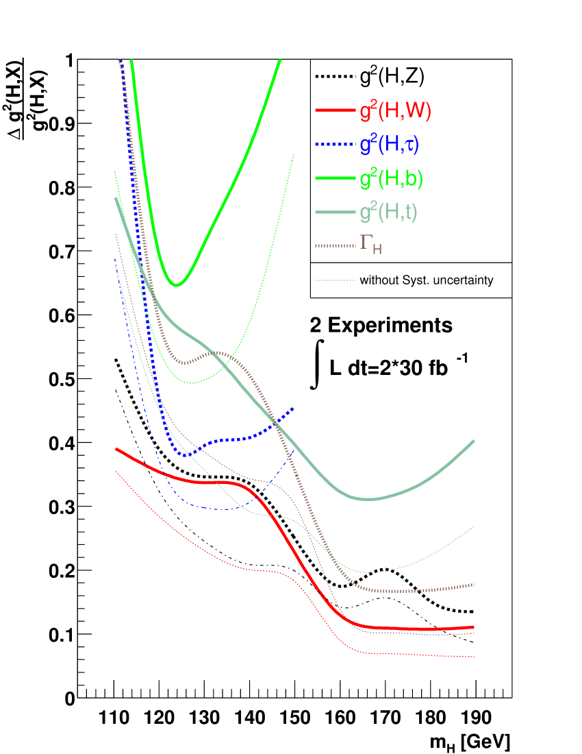
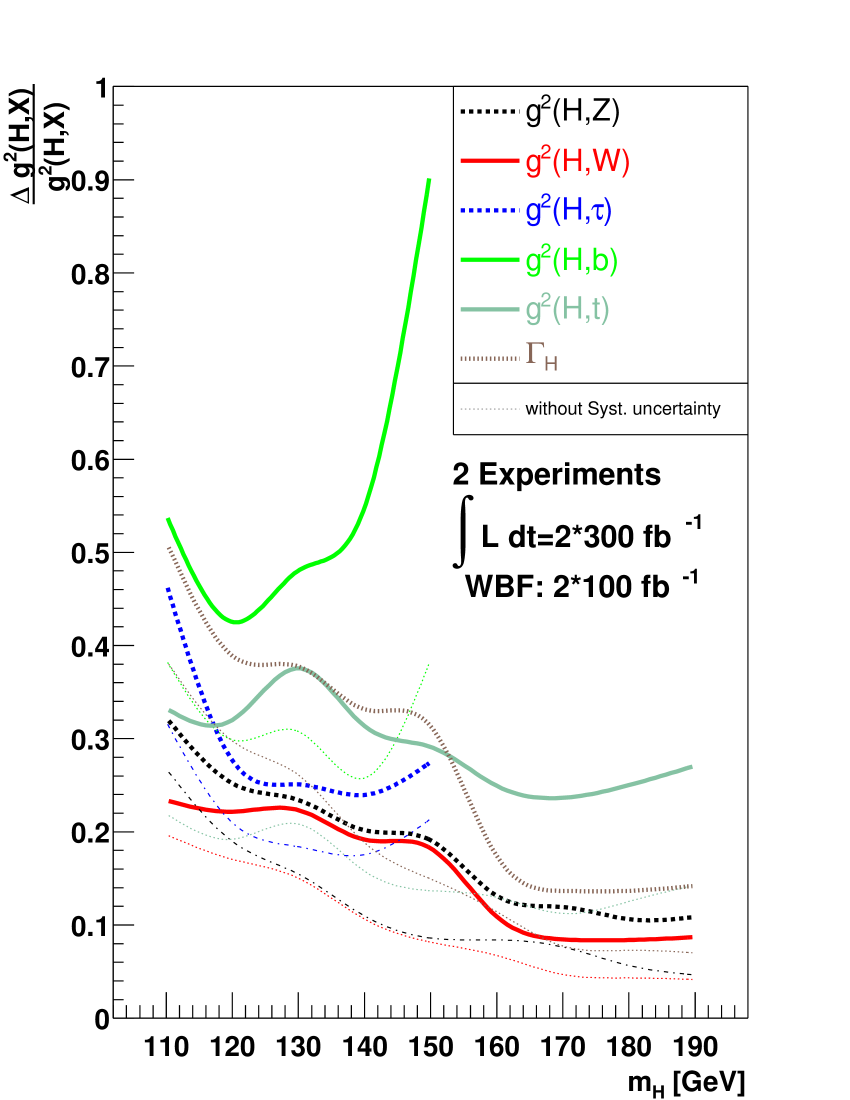
Figure 1: Relative precisions of fitted Higgs couplings-squared as a function of $m_{H}$ assuming SM rates in the low (left) and mixed (right) luminosity scenarios. The precisions in the high luminosity scenario are about the same as in the mixed scenario, except that the $\tau$ coupling extraction improves.

Within a particular model, we can ask whether a deviation from the SM is visible in the Higgs boson couplings. In the MSSM, the properties of the lightest Higgs boson $h$ approach those of the SM Higgs in the decoupling limit of large $M_{A}$. We perform a $\chi^{2}$ fit in particular MSSM scenarios to see how far into the decoupling regime $h$ can be distinguished from the SM. Results are shown in Fig. 2 (left) for the $m_{h}^{\rm max}$ scenario. The LHC is surprisingly sensitive: with high luminosity, $h$ can be distinguished from the SM Higgs at the $5\sigma$ level in this scenario out to $M_{A}\simeq 350$ GeV. The sensitivity comes mostly from the WBF channels, as shown in Fig. 2 (right). This shows the importance of trying hard to get the WBF channels to work at high luminosity.

Figure 2: Fit within the MSSM $m_{h}^{\rm max}$ scenario in the $M_{A}$–$\tan\beta$ plane. The region to the left of the curves would yield a $\geq 5\sigma$ ($\Delta\chi^{2}\geq 25$) discrepancy from the SM. The mostly-horizontal dotted lines are contours of $m_{h}$ in steps of 5 GeV. (Left) $\Delta\chi^{2}=25$ contours in the low (solid line), mixed (long-dashed), and high (short-dashed) luminosity scenarios. (Right) $\Delta\chi^{2}=25$ contours in the high luminosity scenario using WBF channels only (long-dashed), all channels except WBF (short-dashed), and the full fit (solid line).

4 Acknowledgements

I thank M. Dührssen, S. Heinemeyer, D. Rainwater, G. Weiglein and D. Zeppenfeld for a fruitful collaboration leading to the paper [?] on which this talk was based. This work was supported in part by the U.S. Department of Energy under grant DE-FG02-95ER40896 and in part by the Wisconsin Alumni Research Foundation.

References

- [1] D. Zeppenfeld, R. Kinnunen, A. Nikitenko and E. Richter-Was, Phys. Rev. D 62, 013009 (2000); A. Djouadi et al., hep-ph/0002258.
- [2] A. Belyaev and L. Reina, JHEP 0208, 041 (2002).
- [3] M. Dührssen, S. Heinemeyer, H. Logan, D. Rainwater, G. Weiglein and D. Zeppenfeld, hep-ph/0406323; K. A. Assamagan et al., hep-ph/0406152.
- [4] M. Dührssen, ATL-PHYS-2003-030, available from http://cdsweb.cern.ch .
- [5] O. J. P. Eboli and D. Zeppenfeld, Phys. Lett. B 495, 147 (2000).