A QCD dipole formalism for forward-gluon production

Abstract

We derive inclusive and diffractive forward-gluon production in the scattering of a $q\bar{q}$ dipole off an arbitrary target in the high-energy eikonal approximation, suitable to study the saturation regime. We show how the inclusive cross-section is related to the total cross-section for the scattering of a colorless pair of gluons on the target: the gluon-production cross-section can be expressed as a convolution between this $gg$ dipole total cross-section and a dipole distribution. We then consider as an application the forward-jet production from an incident hadron and describe forward-jet production at HERA and Mueller-Navelet jets at Tevatron or LHC. We show how these measurements are related to the $q\bar{q}-gg$ or $gg-gg$ dipole-dipole cross-sections and why they are therefore well-suited for studying high-energy scattering in QCD.

I Introduction

Understanding high-energy scattering in QCD has been the purpose of a lot of work over the past ten years. At high energies, as one approaches the unitarity limit, high-density phases of partons are created and non-linear effects become important. In this regime called saturation glr ; glr+ ; mv ; jimwlk ; bk ; bk+ ; golec , the basic properties of perturbative QCD, such as factorization and linear evolution, breakdown. To study scattering near the unitarity limit, the $q\bar{q}$ dipole model dipole ; mueller has been developed. This formalism constructs the light-cone wavefunction of a dipole (a quark-antiquark pair in the color singlet state) in the leading logarithmic approximation. The size of the dipole provides a scale which is supposed to be much smaller than $1/\Lambda_{QCD}$ to justify the use of perturbation theory. As the energy increases, the dipole evolves and the wavefunction of this evolved dipole is described as a system of elementary dipoles. This formalism is well-suited to study high-energy scattering because when this system of dipoles scatters on a target, density effects and non-linearities that lead to saturation and unitarization of the scattering amplitude can be taken into account.

On a phenomenological point of view, the key point is to relate the experimental probes to the scattering of a dipole. In the case of lepton-hadron collisions this is straightforward: a lepton undergoes hadronic interactions via a virtual photon and one can view the interation as the splitting of the virtual photon into a $q\bar{q}$ pair which then interacts. This dipole picture has had great succes for the phenomenology of hard processes initiated by virtual photons. In hadron-hadron collisions however, there are no such virtual-photon probes. The probes are the final-state particules that we measure, e.g. a final-state gluon that we detect as a jet. Establishing a link between the scattering of a dipole and observables like jet cross-sections is of great theoretical and phenomenological interest in the prospect of the LHC, if one considers the impact that the dipole picture has had on HERA phenomenology for example and how the HERA measurements have helped understanding high-energy scattering.

First steps in this direction were taken in kope where gluon radiation from a quark was calculated. In kovtuch , Kovchegov and Tuchin derived the cross-section for inclusive gluon production in deep inelastic scaterring off a large nucleus. In both cases, the cross-sections are expressed in terms of the scattering of a $gg$ dipole (a gluon-gluon pair in the color singlet state) on the target. It is crucial in kovtuch that the target is a nucleus since they work in an approximation in which all the scatterings on the nucleons happen via one or two-gluon exchanges muelkov . On a phenomenological side, descriptions of Mueller-Navelet jets in marpes and forward jets in mpr are performed in terms of $q\bar{q}$ dipole-$q\bar{q}$ dipole scattering, leading to interesting results and predictions. The key point in these analysis is the description of the jet vertex in terms of $q\bar{q}$ dipoles: it is done using the equivalence between the $k_{T}-$factorization and the dipole factorization. The factorization formula used is therefore not justified when the dipole-dipole cross-section is not $k_{T}-$factorizable which could be the case at high energies.

In this paper, we consider the collision between a $q\bar{q}$ dipole and an arbitrary target and calculate the cross-section for the production of a gluon in the forward direction of the dipole. We work in the eikonal approximation valid for high-energy scattering in which the interaction with the target is described by Wilson lines. We derive formulae for the inclusive and diffractive cross-sections. We express the inclusive cross-section in terms of the scattering of a colorless gluon-gluon pair on the target. We generalize the result of kovtuch , obtaining it in a very different framework and for the scattering off any target. We write the inclusive cross-section in the factorized form given below in equation (40): a convolution between an effective dipole distribution and the total cross-section for the scattering of a $gg$ dipole on the target; such a factorization does not happen for the diffractive cross-section. We obtain a very general formula that includes all numbers of gluon exchanges and non-linear quantum evolution.

We then take another step towards the description of observables in hadronic collisions as we extend our results to the case of an incident hadron instead of an incident $q\bar{q}$ pair. This is done by including linear evolution before the emission of the measured gluon and by using collinear factorization. We thus describe forward-jet cross-sections at hadronic colliders in terms of the scattering of a $gg$ dipole on the target, see later formula (55) which exhibits a dipole factorization for the forward-jet probe and generalizes the formulation of marpes ; mpr .

Finally, as an application to our formulae, we consider the target to be a virtual photon, or equivalently a $q\bar{q}$ dipole, and obtain the forward-jet cross-section at HERA dis . Its high-energy behavior is driven by the quantum evolution of the $gg$ dipole-$q\bar{q}$ dipole scattering, making the forward-jet measurement of particular interest to investigate high-energy scattering and unitarization in QCD. The same conclusion holds for the Mueller-Navelet jet cross-section mnj at Tevatron or LHC that we also derive.

The plan of the paper is as follows. In Section 2, single inclusive forward-gluon production in the scattering of a $q\bar{q}$ dipole off an arbitrary target is calculated. The diffractive cross-section is derived in Section 3. The relation between the inclusive cross-section and the $gg$ dipole-target scattering is derived in Section 4. In section 5, extending the previous result to the case of an incident hadron and specifying different targets, we derive the Mueller-Navelet jet and forward-jet cross-sections. Section 6 concludes.

II Inclusive gluon production

Figure 1: Inclusive gluon production off a $q\bar{q}$ dipole. $x_{0}$ and $x_{1}:$ transverse coordinates of the quark and antiquark; $k$ and $y:$ transverse momentum and rapidity of the measured gluon. The black points represent emission of the gluon by either the quark or the antiquark. The vertical wavy lines represents the interaction with the target. The gluon is emitted before the interaction or after the interaction in which case it comes with a minus sign as explained in the text.

In this section we derive single inclusive gluon production in the high-energy scattering of a $q\bar{q}$ dipole off an arbitrary target. We shall use light-cone coordinates with the incoming dipole being a right mover and work in the light-cone gauge $A_{+}=0.$ In this case, when the dipole passes through the target and interacts with its gauge fields, the dominant couplings are eikonal: the partonic components of the dipole (a quark, an antiquark and soft gluons) have frozen transverse coordinates and the gluon fields of the target do not vary during the interaction. This is justified since the incident dipole propagate at nearly the speed of light and its time of propagation through the target is shorter than the natural time scale on which the target fields vary. The effect of the interaction with the target is that the components of the dipole wavefunction pick up eikonal phases.

Let us be more specific. In Fig.1 is represented the production of a gluon of transverse momentum $k$ and rapidity $y$ off a dipole with transverse coordinates $x_{0}$ for the quark and $x_{1}$ for the antiquark. The size of the dipole $|x_{0}\!-\!x_{1}|$ is supposed to be small in order to justify the use of perturbation theory ($|x_{0}\!-\!x_{1}|\!\ll\!1/\Lambda_{QCD}$). We work in a frame in which the dipole rapidity is not too large so that the radiation of extra softer gluons is to be described by quantum evolution of the target. The necessity of the last term can be seen by considering the case where there are no interactions: the emission-after-interaction term is necessary to get zero gluon production without interaction.

The incident hadronic state is a colorless $q\bar{q}$ pair and has the following decomposition on the Fock states:

$$|d\rangle=|d\rangle_{0}+|dg\rangle_{0}\ .$$ (1)

The bare dipole $|d\rangle_{0}$ is characterised by the wavefunction

$$|d\rangle_{0}=\sum_{\alpha\bar{\alpha}}\frac{\delta_{\alpha,\bar{\alpha}}}{\sqrt{N_{c}}}|(\alpha,x_{0}),(\bar{\alpha},x_{1})\rangle$$ (2)

where $\alpha$ and $\bar{\alpha}$ denote the colors of the quark and antiquark respectively and where the transverse positions of the partons have been specified. The $q\bar{q}g$ part of the dressed dipole $|dg\rangle_{0}$ is characterised by the wavefunction

$$|dg\rangle_{0}=\frac{1}{\sqrt{N_{c}}}\sum_{\alpha\bar{\alpha}\lambda a}\int d^{2}zdy\ \frac{ig_{s}}{\pi}\left[\frac{\epsilon_{\lambda}.(x_{0}\!-\!z)}{|x_{0}\!-\!z|^{2}}-\frac{\epsilon_{\lambda}.(x_{1}\!-\!z)}{|x_{1}\!-\!z|^{2}}\right]T_{\bar{\alpha}\alpha}^{a}|(\alpha,x_{0}),(\bar{\alpha},x_{1}),(a,\lambda,z,y)\rangle\ ,$$ (3)

where the gluon is characterized by its color $a$, its polarization $\lambda$, its rapidity $y$ and its transverse coordinate $z.$ $\epsilon_{\lambda}$ is the transverse component of the gluon polarization vector and $T^{a}$ is a generator of the fundamental representation of $SU(N_{c}).$ The term in brackets in (3) is the well-known wavefunction for the emission of a gluon off a $q\bar{q}$ dipole mueller ; the two contributions correspond to emission by the quark and antiquark respectively. The only assumption made to write down (3) is that the gluon is soft, that is its longitudinal fraction of momentum with respect to the incident dipole is small. As already mentionned, we work in a frame in which only bare or one-gluon components need to be considered in the wavefunction $|d\rangle$; softer gluons will be included through the quantum evolution of the target. One then truncates the perturbative expansion (1) at first order in the strong coupling constant $g_{s}.$

Let us denote the initial state of the target $|t\rangle.$ The outgoing state is obtained from the incoming state $|d\rangle\!\otimes\!|t\rangle$ by action of the ${\cal S}-$matrix. In the eikonal approximation, ${\cal S}$ acts on quarks and gluons as (see for example coursmuel ; kovwie ; heb ):

$${\cal S}|(\alpha,x)\rangle\!\otimes\!|t\rangle=\sum_{\alpha^{\prime}}\left[W_{F}(x)\right]_{\alpha\alpha^{\prime}}|(\alpha^{\prime},x)\rangle\!\otimes\!|t\rangle\ ,\hskip 42.67912pt{\cal S}|(a,\lambda,z,y)\rangle\!\otimes\!|t\rangle=\sum_{b}W_{A}^{ab}(z)|(b,\lambda,z,y)\rangle\!\otimes\!|t\rangle\ ,$$ (4)

where the phase shifts due to the interaction are described by $W_{F}$ and $W_{A},$ the eikonal Wilson lines in the fundamental and adjoint representations respectively, corresponding to propagating quarks and gluons. They are given by

$$W_{F,A}(x)={\cal P}\exp\{ig_{s}\int dz_{+}T_{F,A}^{a}{\cal A}_{-}^{a}(x,z_{+})\}$$ (5)

with ${\cal A}_{-}$ the gauge field of the target and $T_{F,A}^{a}$ the generators of $SU(N_{c})$ in the fundamental ($F$) or adjoint ($A$) representations. ${\cal P}$ denotes an ordering in $z_{+}.$

Therefore the state $|\Psi_{out}\rangle\!=\!{\cal S}|d\rangle\!\otimes\!|t\rangle$ emerging from the eikonal interaction reads $|\Psi_{out}\rangle\!=\!|\Psi_{1}\rangle\!+\!|\Psi_{2}\rangle$ with the componants given by

$$|\Psi_{1}\rangle=\frac{1}{\sqrt{N_{c}}}\sum_{\alpha\bar{\alpha}}\left[W_{F}^{\dagger}(x_{1})W_{F}(x_{0})\right]_{\bar{\alpha}\alpha}|(\alpha,x_{0}),(\bar{\alpha},x_{1})\rangle\otimes|t\rangle\ ,$$ (6)

$$|\Psi_{2}\rangle=\frac{1}{\sqrt{N_{c}}}\sum_{\alpha\bar{\alpha}\lambda b}\int d^{2}zdy\ \frac{ig_{s}}{\pi}\left[\frac{\epsilon_{\lambda}.(x_{0}\!-\!z)}{|x_{0}\!-\!z|^{2}}-\frac{\epsilon_{\lambda}.(x_{1}\!-\!z)}{|x_{1}\!-\!z|^{2}}\right]\left[W_{F}^{\dagger}(x_{1})T^{a}W_{F}(x_{0})\right]_{\bar{\alpha}\alpha}$$

$$W_{A}^{ab}(z)|(\alpha,x_{0}),(\bar{\alpha},x_{1}),(b,\lambda,z,y)\rangle\otimes|t\rangle\ .$$ (7)

$|\Psi_{2}\rangle$ represents the first contribution pictured in Fig.1 while the second contribution is hidden in $|\Psi_{1}\rangle.$ To see that, we must express the Fock states which appear in $|\Psi_{out}\rangle$ in terms of physical states. At first order in $g_{s}$ one has:

$$|(\alpha,x_{0}),(\bar{\alpha},x_{1})\rangle=|(\alpha,x_{0}),(\bar{\alpha},x_{1})\rangle_{phys}-\sum_{\mu\lambda a}\int d^{2}zdy\ \frac{ig_{s}}{\pi}\left[\frac{\epsilon_{\lambda}.(x_{0}\!-\!z)}{|x_{0}\!-\!z|^{2}}T_{\alpha\mu}^{a}|(\mu,x_{0}),(\bar{\alpha},x_{1}),(a,\lambda,z,y)\rangle\right.$$

$$\left.-\frac{\epsilon_{\lambda}.(x_{1}\!-\!z)}{|x_{1}\!-\!z|^{2}}T_{\mu\bar{\alpha}}^{a}|(\alpha,x_{0}),(\mu,x_{1}),(a,\lambda,z,y)\rangle\right]\ ,$$ (8)

$$|(\alpha,x_{0}),(\bar{\alpha},x_{1}),(b,\lambda,z,y)\rangle=|(\alpha,x_{0}),(\bar{\alpha},x_{1}),(b,\lambda,z,y)\rangle_{phys}\ .$$ (9)

One immediately sees that the emission-after-interaction term arises with a minus sign. Dropping the $q\bar{q}$ part which does not conribute to gluon production, using (6), (7), (8), and (9), the outgoing state can be rewritten

$$|\Psi_{out}\rangle=\frac{1}{\sqrt{N_{c}}}\sum_{\alpha\bar{\alpha}\lambda b}\int dy\int d^{2}z\ \frac{ig_{s}}{\pi}\left\{\frac{\epsilon_{\lambda}.(z\!-\!x_{0})}{|z\!-\!x_{0}|^{2}}{\left({\left[W_{F}^{\dagger}(x_{1})T^{a}W_{F}(x_{0})\right]_{\bar{\alpha}\alpha}W_{A}^{ab}(z)-\left[W_{F}^{\dagger}(x_{1})W_{F}(x_{0})T^{b}\right]_{\bar{\alpha}\alpha}}\right)}\right.$$

$$\left.-\frac{\epsilon_{\lambda}.(z\!-\!x_{1})}{|z\!-\!x_{1}|^{2}}{\left({\left[W_{F}^{\dagger}(x_{1})T^{a}W_{F}(x_{0})\right]_{\bar{\alpha}\alpha}W_{A}^{ab}(z)-\left[T^{b}W_{F}^{\dagger}(x_{1})W_{F}(x_{0})\right]_{\bar{\alpha}\alpha}}\right)}\right\}|(\alpha,x_{0}),(\bar{\alpha},x_{1}),(b,\lambda,z,y)\rangle_{phys}\otimes|t\rangle\ .$$ (10)

The different contributions contained in this wavefunction have a straightforward physical meaning: the term containing $\epsilon_{\lambda}.(z\!-\!x_{0})$ comes from the emission of the gluon by the quark while the one containing $\epsilon_{\lambda}.(z\!-\!x_{1})$ comes from to the emission by the antiquark. Moreover for both these terms, the contribution with three Wilson lines corresponds to the interation happening after the gluon emission while the contribution with two Wilson lines corresponds to the interation happening before.

From the outgoing state (10), the gluon-production cross-section reads

$$\frac{d\sigma}{d^{2}kdy}(x_{01})=\frac{1}{2(2\pi)^{3}}\int d^{2}b\sum_{\lambda=\pm}\sum_{c=1}^{N_{c}^{2}-1}\langle\Psi_{out}|a_{c,\lambda}^{\dagger}(k,y)a_{c,\lambda}(k,y)|\Psi_{out}\rangle$$ (11)

where $a_{c,\lambda}^{\dagger}(k,y)$ and $a_{c,\lambda}(k,y)$ are respectively the creation and annihilation operators of a gluon with color $c,$ polarization $\lambda,$ rapidity $y$ and transverse momentum $k.$ $x_{01}\!=\!x_{0}\!-\!x_{1}$ is the size of the incoming dipole and $b\!=\!(x_{0}\!+\!x_{1})/2$ is the impact parameter. Let us rewrite the cross-section (11) using operators $a_{c,\lambda}(z,y)$ in transverse coordinate space that act on $|\Psi_{out}\rangle:$

$$\begin{array}[]{lll}\displaystyle\frac{d\sigma}{d^{2}kdy}(x_{01})&\displaystyle=\frac{1}{4\pi}\int d^{2}b\ \frac{d^{2}z_{1}}{2\pi}\frac{d^{2}z_{2}}{2\pi}\ e^{ik.(z_{2}\!-\!z_{1})}\sum_{\lambda,c}\langle\Psi_{out}|a_{c,\lambda}^{\dagger}(z_{2},y)a_{c,\lambda}(z_{1},y)|\Psi_{out}\rangle\\ \\ &\displaystyle=\frac{\alpha_{s}}{\pi^{2}N_{c}}\int d^{2}b\ \frac{d^{2}z_{1}}{2\pi}\frac{d^{2}z_{2}}{2\pi}\ e^{ik.(z_{2}\!-\!z_{1})}\langle t|P(x_{0},x_{1},z_{1},z_{2})|t\rangle\ .\end{array}$$ (12)

$z_{1}$ and $z_{2}$ represent now the transverse coordinates of the measured gluon in the amplitude and the complex conjugate amplitude respectively. $P(x_{0},x_{1},z_{1},z_{2})$ can be easily calculated from (10) and its definition (12) using

$$\begin{array}[]{lll}\displaystyle a_{c,\lambda}(z,y)|(\alpha,x_{0}),(\bar{\alpha},x_{1}),(c^{\prime},\lambda^{\prime},z^{\prime},y^{\prime})\rangle\!=\!\delta_{cc^{\prime}}\delta_{\lambda\lambda^{\prime}}\delta^{(2)}(z\!-\!z^{\prime})\delta(y\!-\!y^{\prime})|(\alpha,x_{0}),(\bar{\alpha},x_{1})\rangle\ ,\\ \\ \displaystyle\langle(\alpha^{\prime},x_{0}),(\bar{\alpha}^{\prime},x_{1})|(\alpha,x_{0}),(\bar{\alpha},x_{1})\rangle=\delta_{\alpha\alpha^{\prime}}\delta_{\bar{\alpha}\bar{\alpha}^{\prime}}\ .\end{array}$$ (13)

It is given by

$$P(x_{0},x_{1},z_{1},z_{2})=\mbox{Tr}\left[\left\{\frac{x_{0}\!-\!z_{2}}{|x_{0}\!-\!z_{2}|^{2}}{\left({\left[W_{F}^{\dagger}(x_{0})T^{c}W_{F}(x_{1})\right]W_{A}^{*cb}(z_{2})-\left[T^{b}W_{F}^{\dagger}(x_{0})W_{F}(x_{1})\right]}\right)}\right.\right.$$

$$\left.-\frac{x_{1}\!-\!z_{2}}{|x_{1}\!-\!z_{2}|^{2}}{\left({\left[W_{F}^{\dagger}(x_{0})T^{c}W_{F}(x_{1})\right]W_{A}^{*cb}(z_{2})-\left[W_{F}^{\dagger}(x_{0})W_{F}(x_{1})T^{b}\right]}\right)}\right\}$$

$$.\left\{\frac{x_{0}\!-\!z_{1}}{|x_{0}\!-\!z_{1}|^{2}}{\left({\left[W_{F}^{\dagger}(x_{1})T^{a}W_{F}(x_{0})\right]W_{A}^{ab}(z_{1})-\left[W_{F}^{\dagger}(x_{1})W_{F}(x_{0})T^{b}\right]}\right)}\right.$$

$$\left.\left.-\frac{x_{1}\!-\!z_{1}}{|x_{1}\!-\!z_{1}|^{2}}{\left({\left[W_{F}^{\dagger}(x_{1})T^{a}W_{F}(x_{0})\right]W_{A}^{ab}(z_{1})-\left[T^{b}W_{F}^{\dagger}(x_{1})W_{F}(x_{0})\right]}\right)}\right\}\right].$$ (14)

This expression contains terms with four, five, or six Wilson lines, however it can be reduced quite easily using the following formulae:

$$\mbox{Tr}{\left({W_{F}^{\dagger}(x)T^{a}W_{F}(x)T^{b}}\right)}W_{A}^{ab}(z)=\frac{1}{2}\mbox{Tr}{\left({W_{A}^{\dagger}(x)W_{A}(z)}\right)},$$ (15)

$$\mbox{Tr}{\left({W_{F}(x_{1})T^{a}W_{F}^{\dagger}(x_{1})W_{F}(x_{0})T^{a}W_{F}^{\dagger}(x_{0})}\right)}=\frac{1}{2}\mbox{Tr}{\left({W_{A}^{\dagger}(x_{1})W_{A}(x_{0})}\right)}\ .$$ (16)

These are obtained using the Fierz identity that relates the Wilson lines $W_{F}$ and $W_{A}:$

$$\left[W_{F}(x)\right]_{ij}[W_{F}^{\dagger}(x)]_{kl}=\frac{1}{N_{c}}\ \delta_{il}\delta_{jk}+2W_{A}^{ab}(x)T^{a}_{il}T^{b}_{kj}\ .$$ (17)

In formula (14), terms which a priori contain six Wilson lines reduce to traces of two adjoint Wilson lines as $W_{F}^{\dagger}(x)W_{F}(x)=1.$ For the same reason, terms which display five Wilson lines contain only three and can be reduced using (15). Finally, terms with four Wilson lines are either trivial and equal to $C_{F}N_{c}$ or can be reduced using (16). At the end, the cross-section (12) obtained from $P(x_{0},x_{1},z_{1},z_{2})$ contains only traces of two adjoint Wilson lines and is given by

$$\frac{d\sigma}{d^{2}kdy}(x_{01})=\frac{\alpha_{s}}{2\pi^{2}N_{c}}\int d^{2}b\int\frac{d^{2}z_{1}}{2\pi}\frac{d^{2}z_{2}}{2\pi}\ e^{ik.(z_{2}\!-\!z_{1})}\sum_{i,j=0}^{1}(-1)^{i+j}\frac{(x_{i}\!-\!z_{1}).(x_{j}\!-\!z_{2})}{|x_{i}\!-\!z_{1}|^{2}|x_{j}\!-\!z_{2}|^{2}}\left\{\left\langle\mbox{Tr}{\left({W_{A}^{\dagger}(x_{j})W_{A}(x_{i})}\right)}\right\rangle_{t}\right.$$

$$\left.-\left\langle\mbox{Tr}{\left({W_{A}^{\dagger}(x_{j})W_{A}(z_{1})}\right)}\right\rangle_{t}-\left\langle\mbox{Tr}{\left({W_{A}^{\dagger}(z_{2})W_{A}(x_{i})}\right)}\right\rangle_{t}+\left\langle\mbox{Tr}{\left({W_{A}^{\dagger}(z_{2})W_{A}(z_{1})}\right)}\right\rangle_{t}\right\}$$ (18)

where we have denoted $\langle t|\ .\ |t\rangle\!=\!\langle\ .\ \rangle_{t}.$

Interestingly enough, the only quantity involved in (18) is the forward scattering amplitude of a colorless pair of gluons on the target:

$$T(x,x^{\prime},Y\!-\!y)=1-\frac{1}{N_{c}^{2}\!-\!1}\left\langle\mbox{Tr}{\left({W_{A}^{\dagger}(x^{\prime})W_{A}(x)}\right)}\right\rangle_{t}\ .$$ (19)

This scattering amplitude is present in (18) for all the dipoles involved in the process. It contains the scatterings with all numbers of gluon exchanges and, via its quantum evolution, it also contains the emissions of gluons softer than the measured one $(k,y).$ Indeed, if $Y$ is the total rapidity, the amplitude (19) depends on $Y\!-\!y.$ The cross-section (18) is made of four contributions, each of them proportional to one of the $(x_{i}\!-\!z_{1}).(x_{j}\!-\!z_{2})$ ($i,j=0,1$), for which the gluon is emitted from the (anti)quark at transverse coordinate $x_{i}$ in the amplitude and $x_{j}$ in the complex conjugate amplitude. Each contribution itself contains four amplitudes $T$ whose physical origins are the following: $T(x_{i},x_{j},Y\!-\!y)$ corresponds to the gluon being emitted after the interaction both in the amplitude and in the complex conjugate amplitude in which case it does not interact; $T(x_{i},z_{2},Y\!-\!y)$ corresponds to emissions after the interaction in the amplitude and before the interaction in the complex conjugate amplitude and vice-versa for $T(z_{1},x_{j},Y\!-\!y);$ finally $T(z_{1},z_{2},Y\!-\!y)$ corresponds to emissions before the interaction both in the amplitude and in the complex conjugate amplitude.

The scattering amplitude $T(x,x^{\prime},Y\!-\!y)$ is related to the total cross-section $\sigma_{(gg)t}(x\!-\!x^{\prime},Y\!-\!y)$ for the scattering of a gluon dipole $(gg)$ of size $x\!-\!x^{\prime}$ on the target, with rapidity $Y\!-\!y$:

$$\sigma_{(gg)t}(x\!-\!x^{\prime},Y\!-\!y)=2\int d^{2}{\left({\frac{x\!+\!x^{\prime}}{2}}\right)}T(x,x^{\prime},Y\!-\!y)\ .$$ (20)

To compute this cross-section, one has to evaluate the target averaging $\langle\ .\ \rangle_{t}$ contained in $T$ (see formula (19)) which amounts to calculating averages of Wilson lines in the target wavefunction. A lot of studies are devoted to this problem as we briefly discuss later in Section V. Here we only establish the link between the observable (18) and the dipole amplitude (19).

Formula (18) generalizes the result of kovch ; kovtuch where the same cross-section has been derived for a target nucleus in the quasi-classical approximation of muelkov in which the scatterings on each nucleon happen via one or two gluon exchanges. It is quite remarkable that only one dynamical quantity appears in the result and this is what will allow us to write the inclusive cross-section (18) in a factorized form as is shown in Section 4. But first, we shall calculate the diffractive gluon-production cross-section to exhibit the difference with the inclusive one and see that in this case, more than one dynamical quantity is involved.

III Diffractive gluon production

Figure 2: Diffractive gluon production off a $q\bar{q}$ dipole. The object exchanged between the $q\bar{q}$ pair and the target is a color singlet and the target does not break up. Notations: see Fig.1.

The diffractive cross-section for gluon production in a $q\bar{q}$ dipole-target collision is pictured in Fig.2 where we define the diffractive process as one in which the outgoing wavefunction is in a color singlet state and in which the target does not break up. The cross-section is calculated in the same way than the inclusive one in the previous section. The difference is that we now have to project the outgoing state $|\Psi_{out}\rangle$ on the subspace of color-singlet states. The final state containing diffractive gluon production is $|\Psi_{sing}\rangle\!=\!P_{sing}|\Psi_{out}\rangle$ where the projector on the color-singlet states $P_{sing}$ is given by:

$$P_{sing}=\frac{1}{N_{c}}\int d^{2}x\ d^{2}x^{\prime}{\left({\sum_{\mu,\nu}\delta_{\mu,\nu}|(\mu,x),(\nu,x^{\prime})\rangle}\right)}{\left({\sum_{\alpha,\bar{\alpha}}\delta_{\alpha,\bar{\alpha}}\langle(\alpha,x),(\bar{\alpha},x^{\prime})|}\right)}+\frac{1}{C_{F}N_{c}}\sum_{\lambda}\int d^{2}x\ d^{2}x^{\prime}\ d^{2}zdy$$

$${\left({\sum_{\mu,\nu,b}T^{b}_{\nu\mu}|(\mu,x),(\nu,x^{\prime}),(b,\lambda,z,y)\rangle}\right)}{\left({\sum_{\alpha,\bar{\alpha},a}T^{a}_{\alpha\bar{\alpha}}\langle(\alpha,x),(\bar{\alpha},x^{\prime}),(a,\lambda,z,y)|}\right)}\ .$$ (21)

One obtains with (6), (7), and (21):

$$P_{sing}|\Psi_{1}\rangle=\frac{1}{N_{c}}\mbox{Tr}{\left({W_{F}^{\dagger}(x_{1})W_{F}(x_{0})}\right)}|d\rangle_{0}\otimes|t\rangle\ ,$$ (22)

$$P_{sing}|\Psi_{2}\rangle=\frac{1}{C_{F}N_{c}}\frac{1}{\sqrt{N_{c}}}\sum_{\alpha\bar{\alpha}\lambda a}\int d^{2}zdy\ \frac{ig_{s}}{\pi}\left[\frac{\epsilon_{\lambda}.(x_{0}\!-\!z)}{|x_{0}\!-\!z|^{2}}-\frac{\epsilon_{\lambda}.(x_{1}\!-\!z)}{|x_{1}\!-\!z|^{2}}\right]\mbox{Tr}{\left({W_{F}^{\dagger}(x_{1})T^{b}W_{F}(x_{0})T^{c}}\right)}W_{A}^{bc}(z)$$

$$T^{a}_{\bar{\alpha}\alpha}|(\alpha,x_{0}),(\bar{\alpha},x_{1}),(a,\lambda,z,y)\rangle\otimes|t\rangle\ .$$ (23)

$P_{sing}|\Psi_{2}\rangle$ is the contribution of the emission-before-interaction term (first graph in Fig.2). Writing $|d\rangle_{0}\!=\!|d\rangle\!-\!|dg\rangle_{0}$ in $P_{sing}|\Psi_{1}\rangle$ makes the emission-after-interaction term arise (second graph in Fig.2). One is then able to express $|\Psi_{sing}\rangle$ in terms of physical states. Keeping only the $q\bar{q}g$ part, one has:

$$|\Psi_{sing}\rangle=\frac{1}{\sqrt{N_{c}}}\sum_{\alpha\bar{\alpha}\lambda a}\int d^{2}zdy\ \frac{ig_{s}}{\pi}\left[\frac{\epsilon_{\lambda}.(x_{0}\!-\!z)}{|x_{0}\!-\!z|^{2}}-\frac{\epsilon_{\lambda}.(x_{1}\!-\!z)}{|x_{1}\!-\!z|^{2}}\right]\left\{\frac{1}{C_{F}N_{c}}\mbox{Tr}{\left({W_{F}^{\dagger}(x_{1})T^{b}W_{F}(x_{0})T^{c}}\right)}W_{A}^{bc}(z)\right.$$

$$\left.-\frac{1}{N_{c}}\mbox{Tr}{\left({W_{F}^{\dagger}(x_{1})W_{F}(x_{0})}\right)}\right\}T^{a}_{\bar{\alpha}\alpha}|(\alpha,x_{0}),(\bar{\alpha},x_{1}),(a,\lambda,z,y)\rangle_{phys}\otimes|t\rangle\ .$$ (24)

$|\Psi_{sing}\rangle$ is not exactly the final state one needs to consider since our definition of diffractive implies that the target does not break up and we have imposed that condition yet. The final state (24) would be the one to use to calculate diffractive gluon production without any requirement on the target. To insure the target not to break up, one projects the outgoing state $|\Psi_{sing}\rangle$ on the subspace spanned by $|t\rangle.$ The effect is that the Wilson lines in (24) become target-averaged:

$$|\Psi_{diff}\rangle=|t\rangle\langle t||\Psi_{sing}\rangle=\frac{1}{C_{F}N_{c}\sqrt{N_{c}}}\sum_{\alpha\bar{\alpha}\lambda a}\int d^{2}zdy\ \frac{ig_{s}}{\pi}\left[\frac{\epsilon_{\lambda}.(x_{0}\!-\!z)}{|x_{0}\!-\!z|^{2}}-\frac{\epsilon_{\lambda}.(x_{1}\!-\!z)}{|x_{1}\!-\!z|^{2}}\right]\hskip 85.35826pt$$

$$\times\Phi(z)T^{a}_{\bar{\alpha}\alpha}|(\alpha,x_{0}),(\bar{\alpha},x_{1}),(a,\lambda,z,y)\rangle_{phys}\otimes|t\rangle\$$ (25)

with

$$\Phi(z)=\left\langle\mbox{Tr}{\left({W_{F}^{\dagger}(x_{1})T^{a}W_{F}(x_{0})T^{b}}\right)}W_{A}^{ab}(z)\right\rangle_{t}-C_{F}\left\langle\mbox{Tr}{\left({W_{F}^{\dagger}(x_{1})W_{F}(x_{0})}\right)}\right\rangle_{t}\ .$$ (26)

The diffractive gluon-production cross-section is now obtained from formula (11) with $|\Psi_{diff}\rangle$ instead of $|\Psi_{out}\rangle.$ The final result is

$$\frac{d\sigma^{diff}}{d^{2}kdy}(x_{01})=\frac{\alpha_{s}}{\pi^{2}C_{F}N_{c}^{2}}\int d^{2}b\int\frac{d^{2}z_{1}}{2\pi}\frac{d^{2}z_{2}}{2\pi}\ e^{ik.(z_{2}\!-\!z_{1})}\left[\frac{x_{0}\!-\!z_{1}}{|x_{0}\!-\!z_{1}|^{2}}-\frac{x_{1}\!-\!z_{1}}{|x_{1}\!-\!z_{1}|^{2}}\right].\left[\frac{x_{0}\!-\!z_{2}}{|x_{0}\!-\!z_{2}|^{2}}-\frac{x_{1}\!-\!z_{2}}{|x_{1}\!-\!z_{2}|^{2}}\right]\Phi(z_{1})\Phi^{*}(z_{2})\ .$$ (27)

Note that if one had computed the cross-section with $|\Psi_{sing}\rangle,$ there would have been a global target average at the cross-section level and not averages at the amplitude level as is the case in (27). The first term in (26) is proportional to the elastic ${\cal S}-$matrix for the scattering of a colorless $q\bar{q}g$ triplet on the target while the second term is proportional to the elastic ${\cal S}-$matrix for the scattering of a $q\bar{q}$ dipole. There is then two dynamical quantities playing a role in this diffractive cross-section. This is the main difference compared to the inclusive case in which there was only one.

If one considers that the target is a nucleus, and that each scattering on the nucleons happens via a two-gluon exchange, then the target averages in (26) are computable (see e.g. kovwie ) and one recovers the result of kovch . Formulae (27) and (26) are a generalization to an arbitrary target including all numbers of gluon exchanges.

Let us mention also that, making use of the following identity:

$$2\mbox{Tr}{\left({W_{F}^{\dagger}(x_{1})T^{a}W_{F}(x_{0})T^{b}}\right)}W_{A}^{ab}(z)=\mbox{Tr}{\left({W_{F}^{\dagger}(x_{1})W_{F}(z)}\right)}\mbox{Tr}{\left({W_{F}^{\dagger}(z)W_{F}(x_{0})}\right)}-\frac{1}{N_{c}}\mbox{Tr}{\left({W_{F}^{\dagger}(x_{1})W_{F}(x_{0})}\right)}\ ,$$ (28)

one is able to relate the first term of (26) to the scattering of two dipoles and obtain:

$$\Phi(z)=\frac{1}{2}\left\langle\mbox{Tr}{\left({W_{F}^{\dagger}(x_{1})W_{F}(z)}\right)}\mbox{Tr}{\left({W_{F}^{\dagger}(z)W_{F}(x_{0})}\right)}\right\rangle_{t}-\frac{N_{c}}{2}\left\langle\mbox{Tr}{\left({W_{F}^{\dagger}(x_{1})W_{F}(x_{0})}\right)}\right\rangle_{t}\ .$$ (29)

The first term in $\Phi$ is now proportional to the elastic ${\cal S}-$matrix for the scattering of two $q\bar{q}$ dipoles on the target. What is usualy considered is the scattering off a large nucleus in which case one can justify neglecting the fluctuations and writing

$$\left\langle\mbox{Tr}{\left({W_{F}^{\dagger}(x_{1})W_{F}(z)}\right)}\mbox{Tr}{\left({W_{F}^{\dagger}(z)W_{F}(x_{0})}\right)}\right\rangle_{t}=\left\langle\mbox{Tr}{\left({W_{F}^{\dagger}(x_{1})W_{F}(z)}\right)}\right\rangle_{t}\left\langle\mbox{Tr}{\left({W_{F}^{\dagger}(z)W_{F}(x_{0})}\right)}\right\rangle_{t}\ .$$ (30)

Making this simplification is very useful to do phenomenology munsho , as it enables to deal with only one quantity, but it is not correct for any target. Note also that if one writes the product in the right-hand side of (30) using $T$ amplitudes as in (19), one recovers the two-gluon exchange approximation calculated in bart ; kopdiff by neglecting the $T^{2}$ term.

IV Dipole-factorized form of the inclusive cross-section

We now come back to the case of the inclusive cross-section (18) and show in this section that it can be significantly simplified and expressed in a form that exhibits a dipole factorization.

On the right-hand side of (18), the term in brakets contains four amplitudes and for each of them two of the integrations can easily be carried out. Let us begin with the amplitude which does not depend on $b,$ the integration of the emission kernel over that impact parameter gives:

$$\int d^{2}b\ \frac{(x_{i}\!-\!z_{1}).(x_{j}\!-\!z_{2})}{|x_{i}\!-\!z_{1}|^{2}|x_{j}\!-\!z_{2}|^{2}}=2\pi\log{\frac{\rho}{|x_{ij}\!-\!z_{1}\!+\!z_{2}|}}$$ (31)

where $x_{ij}\!=\!x_{i}\!-\!x_{j}$ and $\rho$ is an infrared cutoff which will eventually disappear. Then one writes:

$$\int\frac{d^{2}z_{1}}{2\pi}\frac{d^{2}z_{2}}{2\pi}\ e^{ik.(z_{2}\!-\!z_{1})}{2\pi}\log{\frac{\rho}{|x_{ij}\!-\!z_{1}\!+\!z_{2}|}}T(z_{1},z_{2},Y\!-\!y)=\frac{1}{2}\int\frac{d^{2}z}{2\pi}\ e^{-ik.z}\log{\frac{\rho}{|x_{ij}\!-\!z|}}\ \sigma_{(gg)t}(z,Y\!-\!y)\ .$$ (32)

Consider now the amplitude which only depends on $z_{1},$ we then perform the $z_{2}$ integration:

$$\int\frac{d^{2}z_{2}}{2\pi}\ e^{ik.(z_{2}\!-\!z_{1})}\frac{(x_{i}\!-\!z_{1}).(x_{j}\!-\!z_{2})}{|x_{i}\!-\!z_{1}|^{2}|x_{j}\!-\!z_{2}|^{2}}=\frac{k.(x_{i}\!-\!z_{1})}{ik^{2}|x_{i}\!-\!z_{1}|^{2}}\ e^{ik.(x_{j}-z_{1})}$$ (33)

and obtain

$$\int d^{2}b\int\frac{d^{2}z_{1}}{2\pi}\frac{k.(x_{i}\!-\!z_{1})}{ik^{2}|x_{i}\!-\!z_{1}|^{2}}\ e^{ik.(x_{j}-z_{1})}T(z_{1},x_{j},Y\!-\!y)=\frac{1}{2}\int\frac{d^{2}z}{2\pi}\ e^{-ik.z}\frac{k.(x_{ij}\!-\!z)}{ik^{2}|x_{ij}\!-\!z|^{2}}\ \sigma_{(gg)t}(z,Y\!-\!y)\ .$$ (34)

One can easily see that the amplitude which only depend on $z_{2}$ gives the same result. For the last amplitude which does not depend either on $z_{1}$ or $z_{2},$ we integrate the emission kernel:

$$\int\frac{d^{2}z_{1}}{2\pi}\frac{d^{2}z_{2}}{2\pi}\ e^{ik.(z_{2}\!-\!z_{1})}\frac{(x_{i}\!-\!z_{1}).(x_{j}\!-\!z_{2})}{|x_{i}\!-\!z_{1}|^{2}|x_{j}\!-\!z_{2}|^{2}}=\frac{1}{k^{2}}\ e^{-ik.x_{ij}}$$ (35)

and the $b$ integration of the amplitude yields to the cross-section. Putting the pieces together, the gluon production cross-section reads

$$\frac{d\sigma}{d^{2}kdy}(x_{01})=\frac{\alpha_{s}C_{F}}{2\pi^{2}}\int\frac{d^{2}z}{2\pi}\ e^{-ik.z}\sum_{i,j=0}^{1}(-1)^{i+j}{\left({\log{\frac{|x_{ij}\!-\!z|}{\rho}}-\frac{2ik.(x_{ij}\!-\!z)}{k^{2}|x_{ij}\!-\!z|^{2}}-\frac{2\pi}{k^{2}}\ \delta^{(2)}(x_{ij}\!-\!z)}\right)}\sigma_{(gg)t}(z,Y\!-\!y)\ .$$ (36)

Performing the summation over $i$ and $j,$ the cutoff $\rho$ disappears and the two terms displaying $\delta^{(2)}(z)$ also vanish because $\sigma_{(gg)t}(0,y)\!=\!0$. Using then the following results for two dimensionnal vectors where $\Theta$ is the Heavyside step function:

$$\int_{0}^{2\pi}d\theta_{x}\log{\frac{|z|^{2}}{|x\!-\!z||x\!+\!z|}}=4\pi\Theta(|x|\!-\!|z|)\log{\frac{|z|}{|x|}}\ ,$$ (37)

$$\int_{0}^{2\pi}d\theta_{x}\ \frac{2i}{k^{2}}{\left({2\frac{k.z}{|z|^{2}}-\frac{k.(z\!-\!x)}{|z\!-\!x|^{2}}-\frac{k.(z\!+\!x)}{|z\!+\!x|^{2}}}\right)}=\frac{8i\pi}{|k||z|}\cos{\theta_{z}}\Theta(|x|\!-\!|z|)\ ,$$ (38)

one carries out the integration over the azimutal angle of $x_{01}.$ Denoting the size of the incident $q\bar{q}$ dipole $|x_{01}|\!\equiv\!r_{0},$ the result reads

$$\frac{d\sigma}{d^{2}kdy}(r_{0})=\frac{\alpha_{s}C_{F}}{\pi^{2}}\int d^{2}z\ e^{-i|k||z|\cos{\theta}}\left\{{\left({\frac{2i}{|k||z|}\cos{\theta}-\log{\frac{r_{0}}{|z|}}}\right)}\Theta(r_{0}\!-\!|z|)+\frac{2}{k^{2}}\delta(z^{2}\!-\!r_{0}^{2})\right\}\sigma_{(gg)t}(z,Y\!-\!y)\ .$$ (39)

Most of the time the cross-section $\sigma_{(gg)t}(z,y)$ will not depend on $\theta$ as one averages over the azimutal angle of the target. This enables the final $\theta$ integration:

$$\frac{d\sigma}{d^{2}kdy}(r_{0})=\frac{2\alpha_{s}C_{F}}{\pi k^{2}}\int dz^{2}\phi(r_{0},z,k)\sigma_{(gg)t}(z,Y\!-\!y)\ .$$ (40)

We have singled out the following normalized distribution:

$$\phi(r_{0},z,k)=\Theta(r_{0}\!-\!z){\left({\frac{k}{z}J_{1}(kz)-\frac{k^{2}}{2}J_{0}(kz)\log(r_{0}/z)}\right)}+J_{0}(kz)\delta(r_{0}^{2}-z^{2})\ ,$$ (41)

$$\int dz^{2}\ \phi(r_{0},z,k)=1\ .$$ (42)

Note that now, $z$ and $k$ respectively stand for $|z|$ and $|k|.$ The gluon production cross-section as written in (40) exhibits a dipole factorization: the $gg$ dipole-target cross-section $\sigma_{(gg)t}$ is convoluted with the effective dipole distribution $\phi$ which contains the emission of the forward jet of momentum $k$ off the initial $q\bar{q}$ dipole of size $r_{0}$. It is remarkable that we obtain factorization and such a simple formula.

One can easily check that $\phi$ (41) verifies:

$$2z\phi(r_{0},z,k)=\frac{\partial}{\partial z}\left[\Theta(r_{0}-z)z\frac{\partial}{\partial z}{\left({J_{0}(kz)\log{\frac{r_{0}}{z}}}\right)}\right]\ .$$ (43)

Thanks to this identity, one can express the gluon production cross-section (40) in another convenient way:

$$\frac{d\sigma}{d^{2}kdy}(r_{0})=\frac{2\alpha_{s}C_{F}}{\pi k^{2}}\int_{0}^{r_{0}}dz\ J_{0}(kz)\log{\frac{r_{0}}{z}}\ \frac{\partial}{\partial z}{\left({z\frac{\partial}{\partial z}\ \sigma_{(gg)t}(z,Y\!-\!y)}\right)}\ .$$ (44)

Formulae (40) and (44) express the single inclusive forward-gluon production cross-section in the scattering of a $q\bar{q}$ dipole off an arbitrary target and are the main results of the paper. The intermediate cross-section $\sigma_{(gg)t}$ for the scattering of a $gg$ dipole on the target includes all multiple scatterings and linear or non-linear quantum evolution. As shown by (19) and (20), it can be computed from a trace of Wilson lines correctly averaged over the target gluon fields.

So far, we have only considered the case where the measured gluon is the closest in rapidity to the dijet coming from the dissociation of the incident $q\bar{q}$ pair. One can extend the result to the case of a gluon measured at a less forward rapidity by including the emissions of harder gluons, emitted before the gluon detected in the final state. To stay consistent with our soft-gluon approximation, this can be done by including leading logarithmic evolution before the emission of the measured gluon. This is quite straightforward if one sticks to linear BFKL evolution which is justified as long as the rapidity of the measured gluon is not to big and non-linearities are negligible. Since the incident particule is a $q\bar{q}$ dipole, this BFKL evolution is the usual dipole evolution from the initial dipole of size $r_{0}$ to the dipole of size $r$ from which the measured gluon is now emitted. In formulae, that amounts to do the substitution:

$$\frac{d\sigma}{d^{2}kdy}(r_{0})\rightarrow\int\frac{d^{2}r}{2\pi r^{2}}\ n(r_{0},r,y)\frac{d\sigma}{d^{2}kdy}(r)$$ (45)

where $n(r_{0},r,y)$ is the number density of dipoles of size $r$ inside the initial dipole of size $r_{0}$ at rapidity $y.$ This quantity was defined in mueller and was shown to satisfy the BFKL equation bfkl . The solution is:

$$n(r_{0},r,y)=2{\int\frac{d\gamma}{2i\pi}}{\left({\frac{r_{0}}{r}}\right)}^{2\gamma}\exp{\left({\frac{2\alpha_{s}C_{F}}{\pi}y\chi(\gamma)}\right)}$$ (46)

where the complex integral runs along the imaginary axis from $1/2\!-\!i\infty$ to $1/2\!+\!i\infty$ and where the BFKL kernel is $\chi(\gamma)=2\psi(1)\!-\!\psi(\gamma)\!-\!\psi(1\!-\!\gamma).$ The substitution (45) gives:

$$\frac{d\sigma}{d^{2}kdy}(r_{0})=\frac{2\alpha_{s}C_{F}}{\pi k^{2}}\int dz\ J_{0}(kz)\tilde{n}(r_{0},z,y)\frac{\partial}{\partial z}{\left({z\frac{\partial}{\partial z}\ \sigma_{(gg)t}(z,Y\!-\!y)}\right)}$$ (47)

where

$$\tilde{n}(r_{0},z,y)={\int\frac{d\gamma}{2i\pi}}{\left({\frac{r_{0}}{z}}\right)}^{2\gamma}\frac{1}{2\gamma^{2}}\exp{\left({\frac{2\alpha_{s}C_{F}}{\pi}y\chi(\gamma)}\right)}\ .$$ (48)

The most natural application to our formulae is a measurement in deep inelastic scattering in which one detects the most closest jet to the dijet coming from the dissociation of the photon in case of formula (44) or a less forward jet for formula (47). Such a measurements would certainly give information on the dipole-proton scattering. However the rest of our study will not concentrate on that, it will turn to the case of forward jets emitted by hadrons. Such jets represent the most natural probes in hadronic collisions and are a very interesting application to our formulae.

V An application: forward-jet production

In this part we consider the same cross-section as in the previous section, but with the initial particule being a hadron. Indeed in experiments, collisions that procuce jets are proton-lepton or proton-antiproton collisions. Forward jets are jets measured in the forward directions of the hadrons. We cannot compute such processes directly because of the non-perturbative nature of the hadrons. Therefore we start by explaining how to extend the previous result from an incident perturbative $q\bar{q}$ dipole to an incoming hadron. In a second part, we also specify the target and consider a virtual photon, the goal being to describe forward jets in deep inelastic scaterring. We finally generalize to Mueller-Navelet jets at hadron colliders.

V.1 Gluon production off a hadron

In this section we explain how to make the link between the $q\bar{q}$ dipole and the hadron using collinear factorization. Indeed, providing that the transverse momentum of the measured jet is larger than a perturbative scale, forward-jet production is a hard process and obeys collinear factorization. Moreover, since we are dealing with forward jets, the final state gluon has a fraction of longitudinal momentum (with respect to the incident hadron) $x_{J}$ that is never too low, thus there are no small$-x$ effects in the wavefunction of the hadron that could break collinear factorization.

Here is how we proceed. Consider first the cross-section (47) derived in the previous section and take the collinear limit for the incident dipole $r_{0}\mu\!\gg\!1$ where $\mu$ is an arbitrary hard scale called the factorization scale. This limit requires the emission of the gluon to occur at a scale $k\!\sim\!\mu$ much larger than the scale of the initial dipole $1/r_{0}.$ Such a strong ordering between the two scales is indeed what leads to the collinear factorization. Moreover it is justified in this case because we really want to describe the emission of the jet off a hadron which naturally carries a soft scale. In this appropriate limit, $\tilde{n}(r_{0},z,y)$ reduces to:

$$\tilde{n}(r_{0},z,y)={\int\frac{d\gamma}{2i\pi}}\frac{(r_{0}\mu)^{2\gamma}}{2\gamma^{2}}\ \exp{\left({\frac{2\alpha_{s}C_{F}}{\pi}y\chi(\gamma)}\right)}(z\mu)^{-2\gamma}\simeq{\int\frac{d\gamma}{2i\pi}}{\left({r_{0}\mu}\right)}^{2\gamma}\frac{1}{2\gamma^{2}}\exp{\left({\frac{2\alpha_{s}C_{F}}{\pi\gamma}y}\right)}$$ (49)

since for $r_{0}\mu\!\gg\!1$ the integral is determined by the $\gamma\!\simeq\!0$ behavior of the integrand. We have used $\chi(\gamma)\!\simeq\!1/\gamma$ for $\gamma\!\simeq\!0.$ Then one recognizes that the right-hand side of (49) is an integral representation of a modified Bessel function bessel :

$${\int\frac{d\gamma}{2i\pi}}{\left({r_{0}\mu}\right)}^{2\gamma}\frac{1}{2\gamma^{2}}\exp{\left({\frac{2\alpha_{s}C_{F}}{\pi\gamma}y}\right)}=\frac{1}{2}\sqrt{\frac{\pi\log(r_{0}^{2}\mu^{2})}{2\alpha_{s}C_{F}y}}\ I_{1}{\left({2\sqrt{\frac{2\alpha_{s}C_{F}}{\pi}\log(r_{0}^{2}\mu^{2})y}}\right)}.$$ (50)

And (47) reduces finally to:

$$\frac{d\sigma}{d^{2}kdx_{J}}(r_{0})\simeq\frac{1}{2k^{2}x_{J}}\left\{\sqrt{\frac{2\alpha_{s}C_{F}\log(r_{0}^{2}\mu^{2})}{\pi\log(1/x_{J})}}\ I_{1}{\left({2\sqrt{\frac{2\alpha_{s}C_{F}}{\pi}\log(r_{0}^{2}\mu^{2})\log(1/x_{J})}}\right)}\right\}\hskip 56.9055pt$$

$$\times\int dz\ J_{0}(kz)\ \frac{\partial}{\partial z}{\left({z\frac{\partial}{\partial z}\ \sigma_{(gg)t}(z,\Delta\eta)}\right)}$$ (51)

where we have changed the variable $y\!=\!\log{1/x_{J}}$ and defined $\Delta\eta\!=\!Y\!-\!\log{1/x_{J}},$ the rapidity interval between the jet and the target. The factor in brackets in (51) is the gluon distribution function $x_{J}g_{d}(x_{J},\mu^{2})$ inside the incident $q\bar{q}$ dipole of size $r_{0}$ at the Double Leading Logarithmic (DLL) approximation. This is not surprising: we have assumed that the emitted gluon was soft which is responsible for the leading $\log(1/x_{J})$ and we have considered the collinear limit which is responsible for the leading $\log(r_{0}^{2}\mu^{2}).$ Within this DLL approximation, the distribution $g_{d}$ inside the $q\bar{q}$ pair of size $r_{0}$ is the same than the gluon distribution inside a gluon of virtuality $1/r_{0}^{2}$ with $2\ C_{F}$ being the color factor instead of $C_{A}.$ Now the link with the gluon production cross-section off an incident hadron is obvious: the hard part of the cross-section is the same and the hadron appears in the cross-section via its parton distribution function $g_{h}$. One has then

$$\frac{d\sigma^{h\!+\!t\!\rightarrow\!J\!+\!X}}{d^{2}kdx_{J}}=\frac{1}{2k^{2}}\ g_{h}(x_{J},\mu^{2})\int dz\ J_{0}(kz)\ \frac{\partial}{\partial z}{\left({z\frac{\partial}{\partial z}\ \sigma_{(gg)t}(z,\Delta\eta)}\right)}\ .$$ (52)

Note that this formula is only valid at the DLL approximation since we have always taken the emitted gluon to be soft, that is $x_{J}\!\ll\!1.$

A simple way to see that (52) is the correct formula is to consider the case of linear leading-logarithmic BFKL evolution between the jet and the target. In this case $\sigma_{(gg)t}$ obeys $k_{T}-$factorization and can be expressed in terms of the unintegrated distribution in the target $f_{T}:$

$$\sigma_{(gg)t}^{BFKL}(z,\Delta\eta)=\frac{4\alpha_{S}N_{c}}{\pi}\int\frac{d^{2}q}{q^{4}}(1-J_{0}(qz))f_{T}(q,Q_{T},\Delta\eta)$$ (53)

where $Q_{T}$ is a scale characterising the target. Inserting (53) into (52) gives

$$\frac{d\sigma^{h\!+\!t\!\rightarrow\!J\!+\!X}_{BFKL}}{d^{2}kdx_{J}}=\frac{4\alpha_{S}N_{c}}{k^{4}}\ g_{h}(x_{J},\mu^{2})f_{T}(k,Q_{T},\Delta\eta)$$ (54)

and we recover the known BKFL result theo for forward-jet production.

Formula (52) can be written in a very simple factorized form if one considers the cross-section integrated over the transverse momentum of the jet above a given cut $E_{T}:$

$$\frac{d\sigma^{h\!+\!t\!\rightarrow\!J\!+\!X}}{dx_{J}}\equiv\int_{E_{T}^{2}}^{\infty}dk^{2}\frac{d\sigma^{h\!+\!T\!\rightarrow\!J\!+\!X}}{d^{2}kdx_{J}}=g_{h}(x_{J},\mu^{2})\int d^{2}z\ \phi_{J}(z,E_{T})\sigma_{(gg)t}(z,\Delta\eta)\ ,$$ (55)

where the distribution $\phi_{J}$ is related to a bessel function:

$$\phi_{J}(z,E_{T})=\frac{E_{T}}{2\pi z}J_{1}(E_{T}z).$$ (56)

We have assumed that the $gg$ dipole-target cross-section $\sigma_{(gg)t}(z)$ goes to a constant as $z$ goes to infinity fast enough to cancel the edge terms in the integrations by parts. Typically, it works with $\sigma_{(gg)t}(z)\!\sim\!1\!-\!\exp{(-z^{2})}$ or with $\sigma_{(gg)t}(z)\!\sim\!1\!-\!\exp{(-\log^{2}(z))}.$ Formula (55) exhibits the dipole factorization for a forward jet emitted off a hadron. We recover the result obtained from indirect calculations in munpes using the equivalence between the $k_{T}-$factorization and the dipole factorization. The feature that this approach couldn’t reveal in is that it is a $gg$ dipole that has to be considered and not a $q\bar{q}$ dipole. We have also shown here that the dipole factorization is still valid when the cross-section $\sigma_{(gg)t}$ is not $k_{T}-$factorizable, justifying the use of (55) to study saturation effects in forward jets marpes ; mpr .

V.2 Forward jets in deep inelastic scattering

The study of forward jets in deep inelastic scattering represents the most straightforward application of our formula. In such processes, a proton scatters on an electron and a jet is detected in the forward direction of the proton. Therefore the interaction takes place between the proton and a transversally ($T$) or longitudinally ($L$) polarized virtual photon, see Fig.3a. An hadronic interaction with a virtual photon is easily expressed in terms of $q\bar{q}$ dipoles: the photon fluctuates into the quark-antiquark pair which then interacts. The wave functions $\phi_{T}$ and $\phi_{L}$ describing the splitting are well-known. The cross-section is then given by formula (55) with the $gg$ dipole-$q\bar{q}$ dipole cross-section $\sigma_{(gg)d}$ carrying the rapidity dependance and with an extra convolution with $\phi_{T,L}:$

$$\frac{d\sigma^{p\!+\!\gamma^{*}\!\rightarrow\!J\!+\!X}_{T,L}}{dx_{J}}=g_{p}(x_{J},\mu^{2})\int d^{2}rd^{2}z\ \phi_{T,L}(r,Q^{2})\phi_{J}(z,E_{T})\sigma_{(gg)d}(r,z,\Delta\eta)\ .$$ (57)

The virtuality of the photon has been denoted $Q^{2}$ and $E_{T}$ is the cut on the jet transverse momentum. In the regime where $Q\!\sim\!E_{T},$ DGLAP evolution is suppressed and fixed-scale quantum evolution drives the high-energy behavior of the cross-section. This evolution is contained in $\sigma_{(gg)d}$ which is the only unknown quantity in formula (57). It can be obtained by computing a trace of Wilson lines averaged over the fields of the dipole, see formulae (19) and (20); performing the target averages and calculating $\sigma_{(gg)d}$ is however not easy. The color glass condensate theory provides a way of doing it:

$$\left\langle\mbox{Tr}{\left({W_{A}^{\dagger}(x^{\prime})W_{A}(x)}\right)}\right\rangle_{d}(\Delta\eta)=\int{\cal D}[{\cal A}]U_{\Delta\eta}[{\cal A}]\ \mbox{Tr}{\left({W_{A}^{\dagger}[{\cal A}(x^{\prime})]W_{A}[{\cal A}(x)]}\right)}$$ (58)

where $U_{\Delta\eta}[{\cal A}]$ is a functional which specifies the probability to have a given field configuration in the target $q\bar{q}$ dipole. When $\Delta\eta\simeq 0$, there are no extra gluon radiation and the amplitude provides the initial condition to the JIMWLK equation jimwlk that describes how $U_{\Delta\eta}[{\cal A}],$ and thus also the target average (58), varies as one increases the rapidity interval $\Delta\eta.$ A lot of work is employed trying to solve the JIMWLK equation, at least numerically but this is far beyond the scope of this paper. Providing the rapidity interval $\Delta\eta$ is not too high, the JIMWLK equation reduces to the BFKL equation whose solution has been known for years. A first solution valid beyond BFKL has been found in edal but it is only valid as long as the color fields in the two dipoles are weak.

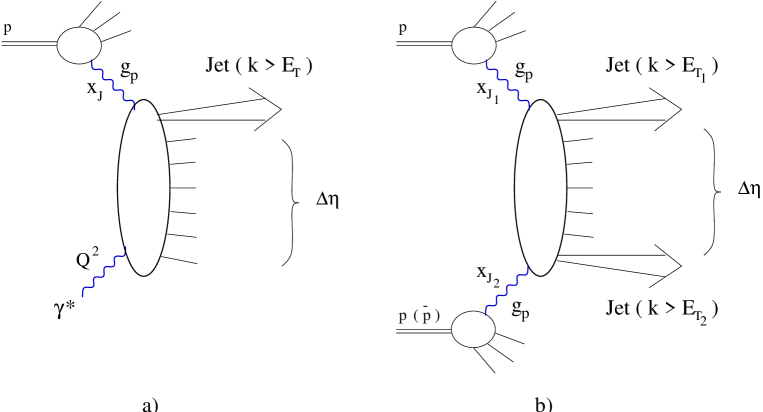
Figure 3: a) Forward-jet production in a proton-lepton collison (at HERA). b) Mueller-Navelet jet production in a proton-proton (at LHC) or proton-antiproton (at Tevatron) collision. $E_{T}$, $E_{T_{1}}$, and $E_{T_{2}}$: cuts on the transverse momenta of the jets; $x_{J},$ $x_{J_{1}},$ and $x_{J_{2}}$: longitudinal momentum fraction of the jets with respect to the incident hadron; $\Delta\eta:$ rapidity intervals between the hard probes.

Anyway, as shown by formula (57), the forward-jet measurement is a suitable observable to study the $gg$ dipole-$q\bar{q}$ dipole scattering and saturation effects purely due to quantum evolution. Forward-jets at HERA seem to be the good candidate to perform the present studies mpr .

V.3 Mueller-Navelet jets at hadron colliders

In the future, Mueller-Navelet jets mnj at LHC could be decisive while at the Tevatron the rapidity range is probably not large enough marpes ; mpr . Mueller-Navelet jets are processes in which a proton strongly interacts with another proton or antiproton and where a jet with a hard transverse momemtum is detected in each of the two forward directions, see Fig.3b. Such processes can also be computed from formula (52): the target is itself a hadron emitting a forward jet. The two cuts on the transverse momenta of the jets will be denoted $E_{T_{1}}$ and $E_{T_{2}}$ and $\Delta\eta$ is now the rapidity interval between the two jets. One has

$$\frac{d\sigma^{p\!+\!p\!\rightarrow\!J\!+\!X+\!J}}{dx_{J_{1}}dx_{J_{2}}}=g_{p}(x_{J_{1}},\mu^{2})g_{p}(x_{J_{2}},\mu^{2})\int d^{2}rd^{2}z\ \phi_{J}(r,E_{T_{1}})\phi_{J}(z,E_{T_{2}})\sigma_{(gg)(gg)}(r,z,\Delta\eta)$$ (59)

and now the cross-section $\sigma_{(gg)(gg)}$ for the scattering of two $gg$ dipoles is the quantity driving the evolution with the rapidity. (57) and (59) are generalizations of the known formulae for forward jets dis and Mueller-Navelet jets mnj that included only linear BFKL evolution. Full quantum evolution is included in (57) and (59) via the $gg$ dipole-$gg$ dipole cross-section. That makes those two measurements suitable observables for studying saturation due to evolution and unitarization of the dipole-dipole scattering, as well as for testing phenomenological models marpes .

VI Conclusions

We have derived inclusive and diffractive forward-gluon production in the scattering of a $q\bar{q}$ dipole off a unspecified target in the high-energy eikonal approximation. We worked in a framework in which the incident $q\bar{q}$ pair is represented by its light-cone wavefunction and in which the interaction with the target is described by Wilson lines that shift the components of the incident wavefunction with eikonal phases. We have also assumed that the emitted gluon was soft so that our results are valid at leading-logarithmic accuracy for this measured gluon. The results are given by formulae (18) and (27) for the inclusive and diffractive cross-sections respectively. All multiple gluon exchanges with the target are included. The measured gluon being always the most-forward gluon with respect to the incident $q\bar{q}$ dipole, quantum evolution is contained in the target-averaged quantities. For the inclusive cross-section, only one such quantity is involved: the forward scattering amplitude of a colorless pair of gluons on the target (19). In the diffractive case however, more complicated $q\bar{q}g$ amplitudes play also a role (26).

In the inclusive case, without specifying the target, we were able to simplify the result (18) and to write the cross-section in the factorized form (40). It expresses the forward-jet cross-section as the convolution between an effective dipole distribution (41) and the $gg$ dipole-target cross-section. The dipole factorization (40) for a forward-jet emission is the equivalent of the usual dipole factorization for a virtual photon: this is a dipole formalism for a hadronic probe.

As a simple application of this result, we described forward jets at hadronic colliders. We extended the result to the case of an incident hadron by including linear evolution before the emission of the measured gluon jet and then by using the collinear factorization properties of QCD. Formula (55) is thus is very simple dipole-factorized cross-section that describes forward jets at HERA, Tevatron or LHC, depending on the target. We finally gave the expression for those forward-jet cross-section (57) and Mueller-Navelet jet cross-section (59). They are written in terms of the $gg$ dipole-$q\bar{q}$ dipole or $gg$ dipole-$gg$ dipole cross-sections which are the quantities that determine the high-energy behavior via their rapidity evolution. We have therefore established a link between two observables measurable at HERA, Tevatron or LHC and dipole-dipole cross-sections which are the basic quantities to study to understand high-energy scattering in QCD, saturation and unitarization due to quantum evolution.

References

• (1) L. V. Gribov, E. M. Levin and M. G. Ryskin, Phys. Rep. 100 (1983) 1.
• (2) A. H. Mueller and J. Qiu, Nucl. Phys. B268 (1986) 427; E. Levin and J. Bartels, Nucl. Phys. B387 (1992) 617.
• (3) L. McLerran and R. Venugopalan, Phys. Rev. D49 (1994) 2233; ibid., (1994) 3352; Phys. Rev. D50 (1994) 2225; A. Kovner, L. McLerran and H. Weigert, Phys. Rev. D52 (1995) 6231; ibid., (1995) 3809; R. Venugopalan, Acta Phys. Polon. B30 (1999) 3731.
• (4) E. Iancu, A. Leonidov and L. McLerran, Nucl. Phys. A692 (2001) 583; Phys. Lett. B510 (2001) 133; E. Iancu and L. McLerran, Phys. Lett. B510 (2001) 145; E. Ferreiro, E. Iancu, A. Leonidov and L. McLerran, Nucl. Phys. A703 (2002) 489; H. Weigert, Nucl. Phys. A703 (2002) 823.
• (5) I. Balitsky, Nucl. Phys. B463 (1996) 99; Y. V. Kovchegov, Phys. Rev. D60 (1999) 034008; Phys. Rev. D61 (2000) 074018.
• (6) E. Levin and K. Tuchin, Nucl. Phys. A691 (2001) 779; Nucl. Phys. A693 (2001) 787; S. Munier and R. Peschanski, Phys. Rev. Lett. 91 (2003) 232001; Phys. Rev. D69 (2004) 034008.
• (7) K. Golec-Biernat and M. Wüsthoff, Phys. Rev. D59 (1998) 014017; Phys. Rev. D60 (1999) 114023.
• (8) N. N. Nikolaev and B. G. Zakharov, Zeit. für. Phys. C49 (1991) 607; Phys. Lett. B332 (1994) 184.
• (9) A. H. Mueller, Nucl. Phys. B415 (1994) 373; A. H. Mueller and B. Patel, Nucl. Phys. B425 (1994) 471; A. H. Mueller, Nucl. Phys. B437 (1995) 107.
• (10) B. Z. Kopeliovich, A. Schaefer and A. V. Tarasov, Phys. Rev. C59, (1999) 1609.
• (11) Yu. V. Kovchegov and K. Tuchin, Phys. Rev. D65, (2002) 074026.
• (12) Yu. V. Kovchegov and A. H. Mueller, Nucl. Phys. B529 (1998) 451.
• (13) C. Marquet and R. Peschanski, Phys. Lett. B587 (2004) 201; C. Marquet, hep-ph/0406111.
• (14) C. Marquet, R. Peschanski and C. Royon, Phys. Lett. B599 (2004) 236.
• (15) A. H. Mueller, Nucl. Phys. Proc. Suppl. B18C (1990) 125; J. Phys. G17 (1991) 1443.
• (16) A. H. Mueller and H. Navelet, Nucl. Phys. B282 (1987) 727.
• (17) A. H. Mueller, Parton Saturation-an overview, hep-ph/0111244.
• (18) A. Kovner and U. Wiedemann, Phys. Rev. D64, (2001) 114002.
• (19) A. Hebecker, Phys. Rept. 331, (2000) 1, and references therein.
• (20) Yu. V. Kovchegov, Phys. Rev. D64, (2001) 114016.
• (21) S. Munier and A. Shoshi, Phys. Rev. D69, (2004) 074022.
• (22) J. Bartels, H. Jung and M. Wüsthoff, Eur. Phys. J. C11, (1999) 111.
• (23) B. Z. Kopeliovich, A. Schaefer and A. V. Tarasov, Phys. Rev. D62, (2000) 0540022.
• (24) L. N. Lipatov, Sov. J. Nucl. Phys. 23, (1976) 338; E. A. Kuraev, L. N. Lipatov and V. S. Fadin, Sov. Phys. JETP 45, (1977) 199; I. I. Balitsky and L. N. Lipatov, Sov. J. Nucl. Phys. 28, (1978) 822.
• (25) G. N. Watson, A treatise on the theory of Bessel functions (Cambridge University Press, 1958).
• (26) J. Bartels, A. De Roeck and M. Loewe, Zeit. für Phys. C54 (1992) 635; W-K. Tang, Phys. lett. B278 (1992) 363; J. Kwiecinski, A. Martin, P. Sutton, Phys.Rev. D46 (1992) 921.
• (27) R. Peschanski, Mod. Phys. Lett. A15 (2000) 1891; S. Munier, Phys. Rev. D63 (2001) 034015.
• (28) E. Iancu and A. H. Mueller, Nucl. Phys. A730 (2004) 460.