ON MASTER INTEGRALS
FOR TWO LOOP BHABHA SCATTERING

Abstract

All scalar master integrals (MIs) for massive 2-loop QED Bhabha scattering are identified. The 2- and 3-point MIs have been calculated in terms of harmonic polylogarithms with the differential equation method. The calculation of 4-point MIs is underway. We sketch some alternative methods which help to solve (mainly) singularities of some MIs.

1 Introduction

Bhabha scattering, $e^{+}e^{-}\to e^{+}e^{-}(n\gamma)$, is used in many accelerators for the determination of luminosity. The NLO corrections in the electroweak model are known[1]. The lack of knowledge of the complete NNLO corrections in massive QED has been one of the major sources of the theoretical error at LEP[2], the other two are light fermion initial state pair production and the hadronic vacuum polarization. Several calculations have been already done to get massive NNLO QED results for Bhabha scattering[3, 4, 5, 6]. The first step in calculations is to identify MIs. For genuine vertices the task has been completed in[3]. The additional 3-point MIs coming from boxes and, more involved, the 4-point MIs themselves are presented for the first time at this conference in the first part of the talk. The second major step includes the evaluation of MIs. This process is underway. Two powerful methods are in use. One is based on a bottom-up approach using differential equations[8]. The other uses Mellin-Barnes representations for the calculation of each MI separately. The (semi)-analytical results are already known for some of the more complicated cases[5]. Further, there is a general numerical method to calculate MIs at fixed kinematical Euclidean points[9].

For our complete set of MIs and the current status of calculations, see[6] and the web page[7]. Here we focus on a presentation of the second part of the talk, namely some alternative cross-checks of analytical results.

2 Some cross-checks of analytical results

2.1 Algebraic relations between IR-divergent MIs

The method of determining MIs, which is realized in the package IdSolver[10], is based on the Laporta-Remiddi (LR) algorithm[11]: it determines and solves an appropriate set of algebraic equations with integration by parts[12] and Lorentz invariance[13] identities. The result is a file, sometimes huge in size, which involves relations among MIs with different powers of propagators and irreducible numerators. Such relations can be used to fix singularities of purely IR divergent MIs. An example is shown in Fig. 1.

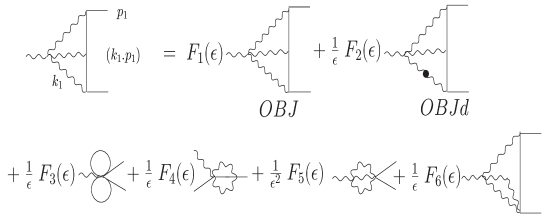
Figure 1: Relation between a vertex ${\it OBJ}$ (here V5l2m2 in terminology of^6,7), the same vertex with a dotted line ${\it OBJd}$ (here V5l2m2d), and with irreducible numerator ($k_{1}p_{1}$).

The diagrams ${\it OBJ}$ and ${\it OBJd}$ are UV finite, but IR divergent. The corresponding diagram with an irreducible numerator is finite. If we expand the known MIs (second row in Fig. 1) into series in $\epsilon=(4-d)/2$ with known coefficients $F_{i}/{\epsilon^{n_{i}}}$, and make an ansatz for the unknowns,

$${\it OBJd}(s) = B_{-2}(s)\frac{1}{\epsilon^{2}}+B_{-1}(s)\frac{1}{\epsilon}+B_{0}(s)+\cdots,$$ (1)

and similarly for ${\it OBJ}$, we get from Fig. 1 relations among the coefficients. Here, e.g. ($a,b,c,d$ are known singularities of the appropriate simpler MIs):

$$0=\frac{1}{\epsilon^{3}}\left[aF_{3}(\epsilon)+bF_{4}(\epsilon)+cF_{5}(\epsilon)+dF_{6}(\epsilon)+F_{2}(\epsilon)B_{-2}(s)\right],$$ (2)

which allows to determine $B_{-2}(s)={1}/{(4s)}$, in agreement with[6]. The crucial point is that there is an additional factor $1/\epsilon$ in front of ${\it OBJd}$ in comparison to ${\it OBJ}$. To get e.g. $B_{-1}(s)$ or $A_{-2}(s)$ (analogous coefficient of ${\it OBJ}$), another equation with a different, independent numerator would have to be used in addition.

2.2 Exact subloop integration

The diagram in Fig. 2 has a massless UV divergent subloop.

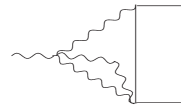
Figure 2: A diagram with a massless propagator subloop.

$$=I=\int\frac{d^{d}k_{1}d^{d}k_{2}}{[k_{2}^{2}][(k_{1}+k_{2}-p_{1})^{2}][k_{1}^{2}+m^{2}][(k_{1}+p2)^{2}]}$$

This allows to perform the subloop integration (over $k_{2}$) analytically, resulting in a $C_{0}$-like function where one of the denominators appears with power $\epsilon$. Using a Feynman parameter representation, after integration over $k_{1}$ and one of the Feynman parameters, we get ($t=(p_{1}+p_{2})^{2}$):

$$I=\pi^{d}\frac{\Gamma(1-\epsilon)^{2}\Gamma(\epsilon)}{16~{}\Gamma(1+\epsilon)^{2}\Gamma(2-2\epsilon)}\epsilon(1+\epsilon)\frac{\Gamma\left(2\epsilon\right)}{\Gamma(2+\epsilon)}I_{num}.$$

This generates a singularity in $I_{num}$ at $x=0$, which can be treated by the following subtraction ($F(x,y)=[(1-x)(1-y)^{2}+xy\frac{t}{m^{2}}]^{-2\epsilon}$):

$$I_{num} = \int_{0}^{1}\frac{dxdy~{}x^{-1+\epsilon}(1-x)^{1-2\epsilon}}{([(1-x)(1-y)^{2}m^{2}+xyt]^{2})^{2\epsilon}}$$

$$= \frac{1}{(m^{2})^{2\epsilon}}\left[\frac{\Gamma(\epsilon)\Gamma(2-2\epsilon)}{\Gamma(2-\epsilon)}\frac{1}{1-4\epsilon}+I_{reg}\right],$$

$$I_{reg} = \int_{0}^{1}dx~{}x^{-1+\epsilon}(1-x)^{1-2\epsilon}\int_{0}^{1}dy\left[F(x,y)-F(0,y)\right].$$

The remaining integrations in $I_{reg}$ can be performed analytically or numerically after the $\epsilon$-expansion:

$$I_{reg} = \int_{0}^{1}dx(1-x)e^{\epsilon\ln x}e^{-2\epsilon\ln(1-x)}\int_{0}^{1}dy\frac{[\ln f(x,y)-\ln f(0,y)]}{x}$$

$$\times~{}\sum_{n=0}^{\infty}(-2\epsilon)^{n}\left[\sum_{k=0}^{n}\ln^{n-k-1}f(x,y)\ln^{k}f(x,0)\right]=I_{1}\epsilon+I_{2}\epsilon^{2}+\cdots$$

In this way both the singularities and also regular terms can be obtained. We have checked that they coincide with our results in[6] and[7] for the MI V4l1m2.

2.3 Subtracting a counter term

The diagram V4l1m1, drawn in bold lines in Fig. 3, is UV divergent.

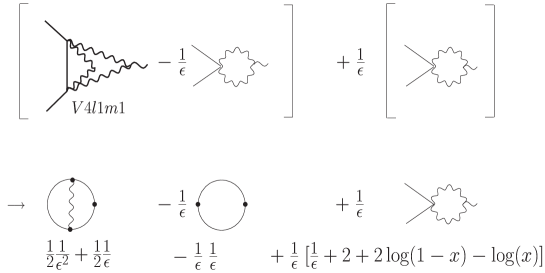
Figure 3: The divergences of the diagram V4l1m1 can be obtained by renormalization theory methods.

Let us introduce a subtraction as in Fig. 3. This subtraction is actually a counter term for the subdivergence in the $\overline{MS}$ scheme. It is known[14] that after such a renormalization of subdivergences the divergences of the result are polynomials in dimensionful parameters. Since the diagram is dimensionless, they are just constants and we can replace massless lines by massive ones and set the external momentum to zero, in this way avoiding spurious IR divergences. This replacement is shown in the second row of Fig. 3 and allows to calculate the singular part of the diagram. For this, we also have to add the subtraction at arbitrary $s$, $x=\frac{\sqrt{-s+4}-\sqrt{-s}}{\sqrt{-s+4}+\sqrt{-s}}$ (second square bracket in Fig. 3). The final result agrees with[6] and[7] for the MI V4l1m1.

2.4 Expressing a subtracted subdiagram by a dispersion relation

The diagram V4l3md contains an IR singular subloop when the dotted line becomes on-shell. After integrating out the UV divergent 2-point subloop, we get

$$I_{V4l3md}=\int\frac{d^{d}k}{[k-p_{1}^{2}-m^{2}]^{2}k^{2}}B_{0}[(k+q)^{2},m^{2},m^{2}].$$ (3)

By subtracting and adding the 2-point subloop as shown schematically in Fig. 4 we get a finite vertex type integral, plus a product of 2-point functions.

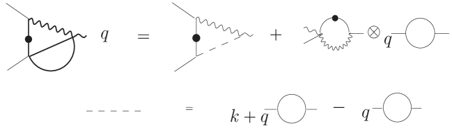
Figure 4: The IR divergent 2-loop diagram V4l3md with a subtraction.

The vertex integral may be further rewritten using a dispersion relation representation for the difference $B_{0}[(k+q)^{2},m^{2},m^{2}]-B_{0}(q^{2},m^{2},m^{2})$ under the integral. After all these preparations, the $\epsilon$ expansion of the diagram may be determined.

Methods like the ones presented in this section are also applicable for 4-point functions.

References

References

- [1] A. Lorca and T. Riemann, hep-ph/0407149, and references therein.
- [2] S. Jadach, hep-ph/0306083.
- [3] R. Bonciani et al., Nucl. Phys. B661 (2003) 289.
- [4] R. Bonciani et al., Nucl. Phys. B681 (2004) 261, Nucl. Phys. B690 (2004) 138.
- [5] V.A. Smirnov, Phys. Lett. B524 (2002) 129; V.A. Smirnov, hep-ph/0406052; G. Heinrich and V.A. Smirnov, hep-ph/0406053.
- [6] M. Czakon, J. Gluza, T. Riemann, hep-ph/0406203.
-
[7]
M. Czakon, J. Gluza, T. Riemann,
http://www-zeuthen.desy.de/theory/research/bhabha/bhabha.html. - [8] A.V. Kotikov, Phys. Lett. B259 (1991) 314; E. Remiddi, Nuovo Cim. A110 (1997) 1435.
- [9] T. Binoth and G. Heinrich, Nucl. Phys. B585 (2000) 741.
- [10] M. Czakon, unpublished.
- [11] S. Laporta and E. Remiddi, Phys. Lett. B379 (1996) 283; S. Laporta, Int. J. Mod. Phys. A15 (2000) 5087.
- [12] K.G. Chetyrkin and F.V. Tkachov, Nucl. Phys. B192 (1981) 159.
- [13] T. Gehrmann and E. Remiddi, Nucl. Phys. B580 (2000) 485.
- [14] J. Collins, Nucl. Phys. B80 (1974) 341; J. Collins, “Renormalization” (Cambridge Univ. Press, 1984).